The outperformance of the semantic learning machine, against commonly used algorithms, for binary and multi-class medical image classification: combined with the usage of feature extraction by several convolutional neural networks

The Outperformance of the Semantic

Learning Machine, Against Commonly

Used Algorithms, for Binary and

Multi-Class Medical Image Multi-Classification

Combined with the Usage of Feature

Extraction By Several Convolutional

Dennis Gerardus Croon

Dissertation presented as the partial requirement for

obtaining a Master's degree in Data Science and Advanced

Analytics

NOVA Information Management School  Instituto Superior de Estatística e Gestão de Informação  Universidade Nova de Lisboa 

The Outperformance of the Semantic Learning Machine, Against Commonly Used Algorithms, for Binary and Multi-Class Medical Image Classification

Combined with the Usage of Feature Extraction By Several Convolutional Neural Networks Dennis Gerardus Croon

Dissertation presented as the partial requirement for obtaining a Master's degree in Data Science and Advanced Analytics

Advisor: Ivo Carlos Pereira Gonçalves

Co-advisor: Mauro Castelli

iv

ACKNOWLEDGEMENTS

First of all, I would like to thank my professors Mauro Castelli and Ivo Gonçalves, who guided the research perfectly, for the infinite patience and faith in my contribution to this promising research. Thanks for developing the Semantic Learning Machine as it currently is. Thanks to NOVA IMS at all for allowing me to widen my horizon by starting at the master’s program which has been such an interesting adventure.

Thanks to my project-members and friends during the first year of the master’s programme for letting me improve myself.

Thanks to all my national and international friends for supporting me during this journey to become a full-stack data scientist and for teaching me some more skills about enjoying life. In particular the smartest and nicest walking data science encyclopaedia that I have ever met, Daniel Cooper. Thank you for advising me during this research, being an amazing guy and teaching me how to catch the waves at Caparica.

At the end a special thanks to my parents and lovely girlfriend Kaja for the trust and belief you had in me all the time throughout this research. You motivated me when things went wrong and you kept believing in me no matter what.

vi

ABSTRACT

Extensive recent research has shown the importance of innovation in medical healthcare, with a focus on Pneumonia. It is vital and lifesaving to predict Pneumonia cases as fast as possible and preferably in advance of the symptoms. An online database source managed to gather Pneumonia-specific image data, with not just the presence of the infection, but also the nature of it, divided in bacterial- and viral infection. The first achievement is extracting valuable information from the X-Ray image datasets. Using several ImageNet pre-trained CNNs, knowledge can be gained from images and transferred to numeric arrays.

This, both binary and multi-class classification data, requires a sophisticated prediction algorithm that recognizes X-Ray image patterns. Multiple, recently performed experiments show promising results about the innovative Semantic Learning Machine (SLM) that is essentially a geometric semantic hill climber for feedforward Neural Networks. This SLM is based on a derivation of the Geometric Semantic Genetic Programming (GSGP) mutation operator for real-value semantics.

To prove the outperformance of the binary and multi-class SLM in general, a selection of commonly used algorithms is necessary in this research. A comprehensive hyperparameter optimization is performed for commonly used algorithms for those kinds of real-life problems, such as: Random Forest, Support Vector Machine, K-NearestNeighbors and Neural Networks.

The results of the SLM are promising for the Pneumonia application but could be used for all types of predictions based on images in combination with the CNN feature extractions.

KEYWORDS

Pneumonia; Semantic Learning Machine; SLM; Convolutional Neural Networks; CNN; Multi-Class Image Predictions; Image Classification; Geometric Semantic Genetic Programming; GSGP

vii

RESUMO

Uma extensa pesquisa recente mostrou a importância da inovação na assistência médica, com foco na pneumonia. É vital e salva-vidas prever os casos de pneumonia o mais rápido possível e, de preferência, antes dos sintomas. Uma fonte on-line conseguiu coletar dados de imagem específicos da pneumonia, identificando não apenas a presença da infecção, mas também seu tipo, bacteriana ou viral. A primeira conquista é extrair informações valiosas dos conjuntos de dados de imagem de raios-X. Usando várias CNNs pré-treinadas da ImageNet, é possível obter conhecimento das imagens e transferi-las para matrizes numéricas.

Esses dados de classificação binários e multi-classe requerem um sofisticado algoritmo de predição que reconhece os padrões de imagem de raios-X. Vários experimentos realizados recentemente mostram resultados promissores sobre a inovadora Semantic Learning Machine (SLM), que é essencialmente um hill climber semântico geométrico para feedforward neural network. Esse SLM é baseado em uma derivação do operador de mutação da Geometric Semantic Genetic Programming (GSGP) para valor-reais semânticos.

Para provar o desempenho superior do SLM binário e multi-classe em geral, é necessária uma seleção de algoritmos mais comuns na pesquisa. Uma otimização abrangente dos hiperparâmetros é realizada para algoritmos comumente utilizados para esses tipos de problemas na vida real, como Random Forest, Support Vector Machine,K-Nearest Neighbors and Neural Networks.

Os resultados do SLM são promissores para o aplicativo pneumonia, mas podem ser usados para todos os tipos de previsões baseadas em imagens em combinação com as extrações de recursos da CNN.

PALAVRAS-CHAVE

Pneumonia; Semantic Learning Machine; SLM; Convolutional Neural Networks; CNN; Multi-Class Image Predictions; Image Classification; Geometric Semantic Genetic Programming; GSGP

viii

INDEX

2. Data extraction from CXRs ... 6

2.1. Data introduction ... 6

2.2. Knowledge using ... 7

2.2.1. Create features ... 8

2.3. Optimizing ML algorithm parameters ... 8

2.3.1. Random Forests ... 10

2.3.2. Support Vector Machine ... 14

2.3.3. K-nearest neighbors ... 19 2.3.4. K neighbors ... 20 2.3.5. Neural Network ... 22 2.3.6. Assumptions ... 24 2.4. Binary CNN comparison ... 25 2.4.1. VGG16 ... 26 2.4.2. VGG19 ... 27 2.4.3. InceptionV3 ... 28 2.4.4. ResNet50 ... 29 2.4.5. InceptionResNetV2 ... 29 2.4.6. Binary summarized ... 30 2.5. Non-binary CNNs ... 31 2.5.1. VGG16 ... 32 2.5.2. VGG19 ... 32 2.5.3. InceptionV3 ... 33 2.5.4. ResNet50 ... 34 2.5.5. InceptionResNetV2 ... 35 2.5.6. Non-binary summarized ... 35 2.6. Conclusion ... 36

ix 3.1. Explained ... 37 3.2. Methodology ... 37 3.3. Experiments ... 38 3.3.1. Binary ... 38 3.3.2. Non-binary ... 39 4. Methodology ... 41 4.1. Data gathering ... 41 4.2. Data pre-processing ... 41 4.3. Experimental setup ... 42

4.4. Semantic Learning Machine ... 42

4.5. Programming methods ... 42

5. Results and discussion ... 44

5.1. Ultimatum ... 45

6. Conclusions ... 47

7. Limitations and recommendations for future works ... 49

8. Bibliography ... 51

9. Annexes ... 54

APPENDIX 1 Binary VGG16 ... 54

APPENDIX 2 Binary VGG19 ... 55

APPENDIX 3 Binary InceptionV3 ... 56

APPENDIX 4 Binary RESNET50 ... 57

APPENDIX 5 Binary InceptionResNetV2 ... 58

APPENDIX 6 Multi-Class VGG16 ... 59

APPENDIX 7 Multi-Class VGG19 ... 60

APPENDIX 8 Multi-Class INCEPTIONV3 ... 61

APPENDIX 9 Multi-Class RESNET50 ... 62

APPENDIX 10 Multi-Class NEURALNETWORK ... 63

APPENDIX 11 Multi-Class INCEPTIONRESNETV2 ... 64

APPENDIX 12 InceptionV3 Architecture ... 65

x

LIST OF FIGURES

Figure 1.1 – Determination of the CTR ... 3

Figure 2.1– CXR Example; Pneumonia (left) and no infection (right) ... 6

Figure 2.2 – Confusion Matrix General ... 9

Figure 2.3 – ROC-curves ... 10

Figure 2.4 – Random Forest ... 11

Figure 2.5 – ROC n_estimators ... 11

Figure 2.6 – Scores max_depth ... 12

Figure 2.7 – Scores min_samples_splits ... 13

Figure 2.8 – Scores min_samples_leafs ... 13

Figure 2.9 – Support Vector Machine [27] ... 14

Figure 2.10 – Scores polynomial degrees ... 15

Figure 2.11- Scores kernels ... 17

Figure 2.12 – Score heatmaps for Gamma against C-value for accuracy (left), AUC (middle) and F-measure (right) ... 18

Figure 2.13 – K-nearest-neighbors method ... 19

Figure 2.14 – Scores k_neighbors ... 20

Figure 2.15 Scores per distance type ... 21

Figure 2.16 – Neural Network ... 23

Figure 2.17 – Receiver Operating Characteristic Curves per algorithm ... 25

Figure 2.18 – Architecture of VGG16 [92] ... 26

Figure 2.19 – Architecture of VGG19 [100] ... 27

Figure 2.20 – Architecture of ResNet50 [25] ... 29

Figure 3.1 – Binary SLM boxplot ... 38

Figure 3.2 – Multi-class SLM Boxplot ... 39

Figure 5.1 – Best performing applications of the SLM ... 45

Figure 9.1– ROC Curve Binary VGG16 ... 54

Figure 9.2 – ROC Curve Binary VGG19 ... 55

Figure 9.3 – ROC Curve Binary InceptionV3 ... 56

Figure 9.4 – ROC Curve Binary ResNet50 ... 57

Figure 9.5 – ROC Curve Binary InceptionResNetV2 ... 58

Figure 9.6 – ROC Curve Multi-Class VGG16 ... 59

Figure 9.7 – ROC Curve Multi-Class VGG19 ... 60

Figure 9.8 – ROC Curve Multi-Class InceptionV3 ... 61

Figure 9.9 – ROC Curve Multi-Class ResNet50 ... 62

Figure 9.10 – ROC Curve Multi-Class Neural Network ... 63

xi Figure 9.12–InceptionV3 Architecture [69] ... 65 Figure 9.13 – InceptionResNetV2 Architecture [200] ... 66

xii

LIST OF TABLES

Table 2.1 – Feature Examples ... 8

Table 2.2 – Optimized RF parameters ... 14

Table 2.3 – Optimized SVM parameters ... 18

Table 2.4 – Scores per weight type ... 22

Table 2.5 – Optimized KNN parameters ... 22

Table 2.6 – Optimized NN parameters by GridSearch ... 24

Table 2.7 – Binary CNN results summary ... 31

Table 2.8 – Non-binary VGG16 results ... 32

Table 2.9 – Non-binary VGG19 results ... 33

Table 2.10 – Non-binary InceptionV3 results ... 33

Table 2.11 – Non-binary ResNet50 results ... 34

Table 2.12 – Non-binary InceptionResNetV2 results ... 35

Table 2.13 – Non-binary results summary ... 36

Table 3.1 – Binary SLM results ... 39

Table 3.2 – Multi-class SLM results ... 40

Table 5.1 – Overview best performing CNN-algorithm combinations ... 44

Table 5.2 – Overview p-values compared with SLM ... 44

Table 9.1 – Overview Binary VGG16 scores ... 54

Table 9.2 – Overview Binary VGG19 scores ... 55

Table 9.3 – Overview Binary InceptionV3 scores ... 56

Table 9.4 – Overview Binary ResNet50 scores ... 57

xiii

LIST OF ABBREVIATIONS AND ACRONYMS

AUC Area Under Curve

CNN Convolutional Neural Network

CV Cross Validation

CXR Chest X-Rays

FPR False Positive Rate

KNN K Nearest Neighbors

NN Neural Network

RF Random Forest

RMSE Root Mean Squared Error

ROC Receiver Operating Characteristic

SLM Semantic Learning Machine

SVM Support Vector Machine

2

1. INTRODUCTION

1.1. PNEUMONIA

The annual incidence of pneumonia amongst children younger than five years of age is 34 to 40 cases per 1000 children in Europe and North America. Higher than at any other time of life, except perhaps with adults older than 75 or 80 years of age [15].

Pneumonia is an infection in at least one lung that can be caused by bacteria, viruses, fungi or parasites. Inflammation in the lung sacs makes it hard to breath and may cause fever and chest pain. The word pneumonia comes from the Greek word “pneumōn” which means lung. The X-ray dataset of pneumonia can be used to predict the existence of alveoli (infected lung sacs) and should determine the pneumonia type. The applied algorithm is reusable for infinite other medical detections and solutions, such as cancer prediction or heart diseases.

1.2. IMPORTANCE

After the pneumonia diagnosis, the patient gets prescribed antibiotics only in case of bacterial infection. Antiviral medication is needed for viral infection, but sometimes a good rest is enough to recover. Only diagnosis and its treatment is an item of expense for the healthcare system: In the US, the direct annual cost of community-acquired pneumonia has been estimated to be at least $17 billion [7], and in Europe, overall annual costs are estimated to be € 10.1 billion [28]. These costs consist of the initial visit and all follow-up visits occurring within 28 days. The costs were based on paid amounts of adjudicated claims, health plan and insurer payments. Total costs were estimated as the sum of all costs in each individual setting [24]. Creating an algorithm that provides advice about the possible infection reduces the costs in the first steps of the health plan: less doctors necessary, less costs for professional opinions. However, the research of Borowska [2] shows us that it is unfeasible thinking about the artificial intelligence taking over the entire healthcare system. Human beings seem to want another one of the same kinds taking care of them at the end, but the steps between could be financially improved. At the end, the work of an Artificial Intelligence (AI) application is proven to be significantly better than the human eye [6].

3

1.3. METHODS

Several methods have been shown in recent articles and researches about applying Machine Learning in medical healthcare. A comparison between the X-ray methods and specific pneumonia applied methods is necessary to determine the benchmark and the bottom line of prediction quality. Besides that, there are multiple ways of implementing image data in the pre-processing phase. The conversion from image to usable input data is hard to understand for the human brain [18].

1.3.1. X-ray

Chest X-rays (CXRs) are the most common and cost-efficient type of medical imaging; it is much easier to consult compared with a CT or MRI scan [6]. The first method used is the organ segmentation in CXRs, hereby the contour of the organs determines abnormal shapes or sizes [8]. The contour and sizes lead directly to the calculation of cardiothoracic ratio (CTR), division of the blue and orange line illustrated in figure 1.1. This is a key clinical indicator, CTR >0.5 suggests an enlargement of the heart. Those types of distinguishable insights could lead to observative knowledge of the used methods.

Besides the fact that it is possible to determine the lung boundaries, the undeveloped adolescent and baby rib cage size should be considered during the training phase of the Machine Learning algorithms [20]. Different algorithms should be applied to the different body shapes to obtain the best prediction of pneumonia cases.

4 The chest is not the only body part where AI is used to advise radiologists. Bone fractures in hands is a similar problem but is solved by using boosting and bagging on the Bayesian Network classifiers [1]. While this has more to do with the outlines of the bones, a probabilistic method is used for each hand section. Ko [13] even used a random forest in their hand fracture data prediction.

1.3.2. Pneumonia

Several ML algorithms have been applied on pneumonia; some determine the seriousness based on biopsies, others use CXRs to predict mortality. Cooper’s research [5] contains more than 40 different properties per patient, such as; blood pressure, heart rate, diabetes, cancer etc. All these combined and applied with multiple algorithms creates a good overview of opportunities. The Neural Networks (NN) and K-Nearest Neighbours (KNN) methods lead to significantly better results. Another example of a biopsy based, pneumonia research, is the one undertaken by Kim [12]. They collected all the biopsy data, cleansed them up and applied a Support Vector Machine (SVM) to the data.This resulted in less than 10% of incorrect predicted values. This might show that SVM is not the best method to find underlaying dependencies when dealing with many different biopsy properties. In this case, the radiologist is better than the SVM.

In order to compete against the radiologist performance, it is proven to use at least a Convolutional Neural Network (CNN) [19]. This CNN is a 121 layer that inputs the CXRs and outputs the probability of pneumonia. A CNN is a specific NN that does not only consider its neighbours around a neuron but can go at least one layer further back than that. This is perfectly feasible for image recognition tasks.

1.4. DATA

In this research we want to prove that it is possible to predict whether pneumonia is present or not. Even though it would be interesting to see the probability or chance of pneumonia per image. The data collected from Kaggle [16] consists of test, train and validation separations, but this will be resampled and split again to prevent luck. Those are divided in “Normal”, that stands for not infected, and “Pneumonia”, that stands for infected. Inside the infected we can choose between bacterial and

5 viral (18444 observations in totally). The goal is to convert the CXRs to filtered and focussed datasets (Chapter 2) and apply them to commonly used algorithms and the Multi-class Semantic Learning Machine (Chapter 3).

6

2. DATA EXTRACTION FROM CXRS

This chapter contains information about the conversion from CXRs to usable input for the SLM. The images’ invaluable data and possible noise should be removed as seen in a recent finger X-ray research [1].

2.1. DATA INTRODUCTION

The X-ray photo illustrated in Figure 2.1 is an example of pneumonia, all of the images have this point of view, but some of them show a slight change around the lungs. Unfortunately, the data does not have a consistency relating to size; this means all of the photos have a different height and width. Inside the Pneumonia cases there is a third labelled separation possible. This means they could be either bacterial or viral. But for now, it is kept binary. This distinction is not necessary for the conversion, but for the training of the SLM and the other considerable algorithms.

After exploring the data, it is time to extract the features from each image. Instead of having an array of 2000x2000 (mean pixels) with each cell filled with a value between 0 and 255 (darkness), we would rather have an array that recognizes and extracts the specific properties of each image. To make this a bit more efficient and sophisticated, we use the knowledge of pre-trained models. The determination of the features is combined with the change to jsonl-format.

7

2.2. KNOWLEDGE USING

There are several pre-trained CNNs for classification and detection created and applicable for this image conversion [11]. The CNNs are tested on a dataset of over 15 million labelled high-resolution images belonging to roughly 22,000 categories; the ImageNet validation set. The chosen ones tested on the validation set are listed below along with the corresponding reason of consideration:

1. VGG16 is the relative older CNN for large scale image recognition

created by Simonyan [22]. The performance on the validation set has a low accuracy compared with the other tested networks, but still has a lot of parameters, which makes it interesting to compare. Besides that, the next point of summation is about a later version of VGG and the curiosity of improvement has been enlarged.

2. VGG19 is, as mentioned before, the later and plausible improved version of VGG16. The difference is implemented in the number of layers, where the number at the end stands for. Instead of 13 convolutional and 3 fully connected layers, the deeper version has 16 and 3 layers respectively. 3. InceptionV3, introducing of the complexity of parallel towers with different filters. The high depth and lower parameters compared with the VGG16, makes it interesting to test against each other. The high top-5 accuracy creates hopeful thoughts about the CXRs conversion.

4. ResNet50 is using shortcut connections, residuals, that decreases the number of layers but is still competing accuracy-wise. Just one fully connected layer is used and that together makes it a completely new interesting network.

5. InceptionResNetV2 is, as it has the appearance of, a combination of the two previous bulky networks. A combination of shortcuts and inception modules; Residual Inception Blocks. Together they have the highest accuracy on the ImageNet validation set.

8

2.2.1. Create features

The python script to generate the clean and resized features of the CXRs dataset is used for summarizing each observation for VGG16, VGG19, Inception, ResNet50 and InceptionResNetV2. A possible structure of the extracted features is listed below.

Table 2.1 – Feature Examples

Dataset features Label

[[[[0.0, 0.0, 0.0, 10, 25, … _Bacterial [[[[0.0, 67.5, 0.0, 0.0, 5, … _Viral [[[[0.0, 0.0, 12.67, 0.0, 0.0, … Normal

The table above shows the extraction from image dataset to arrays of numbers for each label (Bacterial, Viral and Normal). This is an example of the multi-class pre-processing, by changing the Bacterial and Viral data both to “Pneumonia”, the binary dataset is created. The features of each observation, depending on the used CNN, contains a number of layers inside the array (which is recognized by the various starting brackets above). They are flattened down to create a one-dimensional array per observation.

2.3. OPTIMIZING ML ALGORITHM PARAMETERS

I assume that the behaviour of the ML parameters corresponds with the data after the other CNN methods. This is tested in this chapter with the VGG16 featured dataset.

To compare the different algorithms used, consideration of the outcome quality is necessary. Therefor we use various result investigation methods for the comparison between the parameters. The first metric used for result evaluation is accuracy. This gives the first impression about the score of well predicted values as formulated below:

!""#$%"& = )#*+,$ -. /-$$,"0 1$,23"03-45 6-0%7 4#*+,$ -. 1$,23"03-45 *%2,

9 The disadvantage of this measurement is that it only considers the correct predicted values and does not inform about the behaviour of the incorrect predicted ones. To gather more information about the misclassified values, the confusion matrix could be chosen. This provides some more specific information about the classification errors and accuracy per prediction class. An example of a matrix is figured below for a binary classification problem.

Figure 2.2 – Confusion Matrix General

The true negative (TN) and true positive (TP) numbers in the confusion matrix are the correctly classified ones. The sum of this divided by the total number of predictions is equal to the accuracy, but specification of accuracy per predicted binary value is possible. This together with the false positives (FP) and false negatives (FN) gives the overall impression of algorithm quality. To calculate how often predicted true values are correct, the precision formula is implied:

8$,"353-4 = 6$#, 8-53039,

6$#, 8-53039, + ;%75, 8-53039,

To compare the negative prediction over the positive prediction we can use the recall function:

<,"%77 = 6$#, 8-53039,

6$#, 8-53039, + ;%75, ),=%039,

This recall (sensitivity) formula, combined with the specificity formula, creates the base values of the ROC-curve. This curve shows the total distinguished score of a machine learning algorithm. The closer the curve is to the left upper corner, the better the algorithm performs. Two different ROC-curves are shown in Figure 2.3.

10 The comparison between the two curves can be done by calculating the area under curve (AUC). This value between 0 and 1 makes it possible to measure the curves.

Figure 2.3 – ROC-curves

Another way to combine the sensitivity and specificity functions is by using the f-measure.

;_> = ? 2

<,"%77A>_{+ 8$,"353-4}A>B = 2 ∙

8$,"353-4 ∙ <,"%77 8$,"353-4 + <,"%77

This F-measure generates an overall averaged indication about the precision and recall. During the hyperparameter tuning this will be used, paired with the accuracy and area under the curve. These different types of insights create a wide view of algorithm quality.

Besides the quality measurements, a cross validation (CV) is used to avoid invalid results. The 5-fold CV is used to cut the train and test data into five equal sized subsets to create various combinations. The average of those sub-runs will be shown in the graphs in the following paragraphs. This method is used at the background to obtain the most reliable results. All line graphs in this paragraph contain data about the test prediction values, to prevent selection based on overfitting.

2.3.1. Random Forests

The first algorithm to optimize by adjusting the parameters is a Random Forest (RF) algorithm. A RF, illustrated in Figure 2.4, is a combination of a number of different decision trees with a specific range of restrictions. The merging of these multiple Yes/No question-trees leads to a sophisticated tree called a RF. A selection of the

11 RF-settings is tested and optimized in this paragraph. After this phase, the best results combined will be used in the further experiments of this research. Some of the RF parameters are not used in these experiments, because of the big number of features extracted after the CNNs.

Figure 2.4 – Random Forest

N_estimators

The number of different trees used for the total random forest is set as n_estimators. The default parameter value is 100, which introduces the experiment of a range from 0 to 200 (stepwise). In Figure 2.5 the n_estimators (x-axis) is pointed against the score (y-axis). The three different measures, as explained before, are accuracy, AUC and the F-measure.

Figure 2.5 – ROC n_estimators

Figure 2.5 shows the improvement of the complete set of measures, but after a setting of 100 these settings do not have a significant improvement. Hereby the default setting will be chosen for future experiments.

12

Max_depth

The max_depth of each tree, stands for the maximum “height” of each individual decision tree used for the total RF. The deeper the trees, the more splits generated. This could lead to overfitting, the test dataset might not be needing that amount of splits. The default value of this parameter is set as “None”, which means that there is no maximum depth for the trees. In the default case; all the nodes are split out until all leaves contain pure information or when the min_samples_split is not reached anymore. In this experiment, Figure 2.6, max_depth values are chosen from 0 to 30.

Figure 2.6 – Scores max_depth

Unfortunately, this experiment range does not reach the quality measures of the default (dashed line). The deepness of the tree increases all three measures, but by keeping this parameter default (variable) the results will not suffer.

Min_samples_split

This parameter is about the number of samples required to be able to split a node. The lower this value, the more sophisticate the tree is. However, increasing this value may cause underfitting. The nodes won’t achieve enough purity to explain the data correctly. The default setting of this split is set as a value of 2, so a range between 2 and 25 is used for this experiment. The results are figured below.

13 Figure 2.7 – Scores min_samples_splits

Here, the expectations are correct, the higher the minimum of sample splits, the lower the score of the measures. In this case the AUC is significantly decreased. The default value will be used for future testing purposes.

Min_samples_leaf

The number of samples required to be at each leaf node after the split. Logically the split does not give any contribution to the tree if it is split into a leaf of 0 and the residuals to the other one. The higher the minimum samples per leaf, the more difficult it is to apply a split definition. The default value of this parameter is 1, but this experiment shows the results in a range of 1 to 10 (Figure 2.8).

14 Increasing the minimum leaf samples does not result into a higher score in all three measures. There is a slight increase in accuracy and F-measure, but it is not significant enough to take into count for future testing.

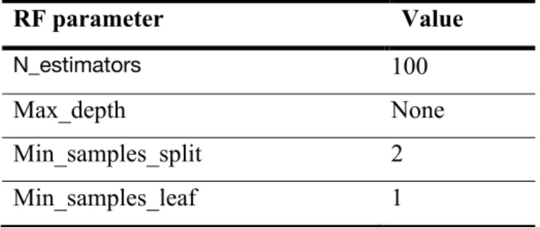
Conclusion

After testing each parameter individually, the parameter settings can be combined together for future experiments. The optimized parameter values are as follows:

Table 2.2 – Optimized RF parameters

RF parameter Value

N_estimators 100

Max_depth None

Min_samples_split 2

Min_samples_leaf 1

2.3.2. Support Vector Machine

The second algorithm to be considered on this pneumonia dataset is called the Support Vector Machine (SVM). This algorithm uses a vector (hyperplane) to separate observations, see Figure 2.9. This vector could have multiple different shapes instead of a straight line. The closest points of each prediction class to the hyperplane is called the support vector. Equally to the RF of previous paragraph, this algorithm has some parameters to optimize either. These will be discussed in the following parts of this paragraph.

15

Kernel

The most influential parameter is the kernel, which is about the shape of separation between the prediction classes. Most SVM graphs are created with the classical straight line, but with this parameter the scientist can chose between ‘polynomial’, ‘linear’, ‘sigmoid’ and ‘rbf’.

Polynomial The concept of polynomial separation is the possibility of creating a

100% clear distinction between the class-points as seen before in Figure 2.9. Applying this to the SVM algorithm creates a higher chance of finding a parameter combination that suits the prepared data.

Inside the polynomial kernel there is an extra dimension available; the degrees. In the formula of the polynomial kernel the part that creates a power calculation is mentioned by the d (degrees).

D(F, &) = (IFJ_{& + ")}K

This number of degrees depends on the data and given the fact that we do not know what the separation between the classes of the pneumonia data looks like, an experiment is necessary. For this occasion, we chose the degree values from 1 to 8 and show the results in Figure 2.10 (same measures as the RF).

The results shown in Figure 2.10 tell that no further research is needed, there is no significant better setting as a degree than the default of 3. This will be the setting for this kernel from this moment on.

16

Linear This understandable type of kernel is mostly used in simple distinguishable

datasets where the scientist only needs to prove the expectations. The function below leads to an infinite line between the classes.

D(F, &) = FJ_{& + "}

Sigmoid The typical wave-shaped kernel (equation below) is known of its use as

an activation function in multiple ML algorithms. The usage of an SVM in combination with this kernel is equivalent for a two-layer, perceptron neural network [3].

D(F, &) = tanh (IFJ_{& + ")}

RBF This exponential Radial Basis Function kernel (figure X), also known as the

Gaussian kernel, is another example of a curved separation between classes. The RBF is a smooth boarder between the two classes and curves among the distances between the hyperplane and the dots.

DPF_Q, F_RS = ,TA

UVWAVXUY

Z[Y \

These kernels are tested with the measures as explained in the previous section. The bar graph in Figure 2.11 shows the results of the kernel experiment. To create a better overview of the gathered results; the score information is written in the coloured bars of the plot. The Sigmoid kernel is significantly worse than the other three. Nevertheless, the Polynomial set with a degree of 3 is scoring consequently better over the measures.

17 Figure 2.11- Scores kernels

Combined tuning

Besides the kernel optimization, the SVM algorithm contains two other influential parameters; gamma and c. Regarding the fact that they are both numeric values, the method to optimize them combined is used in this section.

Gamma The gamma parameter defines the importance of a training example; the

higher this value, the more data-specific the separation between the classes is. The decreased value of gamma leads to a constraint predictive model, it would not adjust to the complexity of the data.

C This second important parameter introduces a penalty to the SVM. The bigger

this error value, the smaller the margin of the hyperplane will be. When you choose to set a small c, misclassification is allowed more, and the margin of the hyperplane would increase.

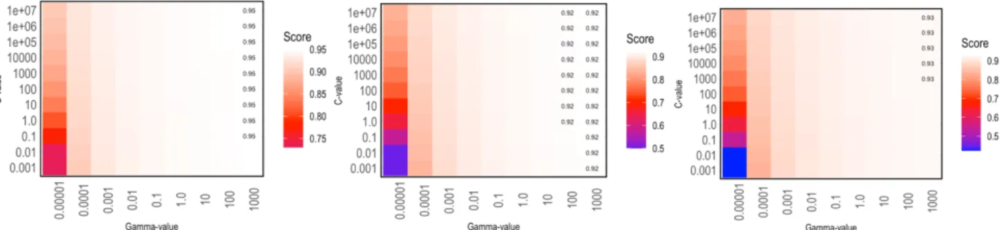
18 The experiment of the gamma and c combined is logarithmically scaled and figured in a heatmap, Figure 2.12, per measure. Both parameters range from tiny to huge with a score per unique combination. Regarding the previous section; the polynomial kernel leads to the best results, so it is set here either.

Figure 2.12 shows significantly higher scores for a relatively high gamma setting. The penalty parameter acts similar to the gamma which results in big combined values. For the best results; the allowance of misclassification increased paired with the high importance (gamma) of the data points. Clearly, there is an importance of a gamma-value set as 1000, while the c parameter could be in a range of 1000 to 1.0xe07_{. The average on the logarithmic scale is taken as optimum: 1.0xe}05_{. Even}

though this experiment is completed with secure cross-validation and data splitting, it is crucial to take into account overfitting for future purposes.

Conclusion

The polynomial kernel with a number of degrees set as 3 shows the highest scores for all three scoring measurements, so this is set as best parameter. A combined experiment for gamma and c result in the values listed in Table 2.3, which are going to be used for future purposes.

Table 2.3 – Optimized SVM parameters

SVM parameter Value

Kernel Polynomial (n=3)

Gamma 1000

C 1.0xe05

Figure 2.12 – Score heatmaps for Gamma against C-value for accuracy (left), AUC (middle) and F-measure (right)

19

2.3.3. K-nearest neighbors

The algorithm that uses, as its title reveals, the neighborhood of points to predict incoming observations is called K-nearest neighbors algorithm (KNN). This algorithm could be applied to cluster and classification applications but will be used as a classification algorithm in this scenario. The intention, figured below, of KNN is to drop the unclassified (test) observations into the field with training observations and determine the class, but this process includes some parameters; e.g. minimum number of neighbors, distance metric and the weight of points in neighborhood.

20

2.3.4. K neighbors

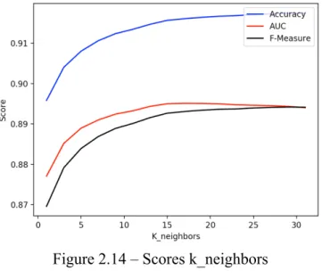
K is the first parameter; the minimum number of neighbors selecting as close as possible. The class will be determined by the majority class of k selected points. To avoid ties an uneven number must be set as k. The experiment range for the number of neighbors will be from 1 to 31 with step size as 2.

The default value is 5, so the improvement is recognizable for all measures in Figure 2.14. The best AUC value is achieved by a number of neighbors of 15. The remaining two measures do not increase significantly in value after this. K_neighbors is set to 15 instead the default 5.

Distance

Some different methods exist to calculate the distance from a point to be determined to the classed surrounded observations. Three options for generating the distance are:

Euclidean distance is the well-known and commonly used metric of calculating the

exact length of the segment connecting two points. Which is given by:

2(F, &) = ]^(F_Q − &_Q)Z `

Qa>

21

Manhatten known as the city block shape distance metric named by the look of the

city blocks. It is impossible to walk straight lined from one point to another but walking along the blocks is the only option. The distance is calculated by:

^|c_d− e_d|

f

dag

Minkowski is a generalised combination of the previous two equations. It results

in a Manhatten version when p = 1 and in a Euclidean equation when p = 2. This normed formula is known as:

T^|c_d− e_d|h i

dag

\

g/h

Comparing the three different distance metrics is done by setting the metric to ‘Minkowski’ and varying the p from 1 to 3. Resulting in the plot below.

Figure 2.15 Scores per distance type

There is no significant difference between the metrics, but slightly higher scores for the Manhattan distance calculation. This will be used for future purposes.

Weights

Besides using the majority of point to classify, the distance to each selected point could be taken into count also. This parameter is called weights; using the uniform weight parameter only considers the majority of classes to determine the prediction. Against the uniform classification method, the distance could be used for

22 generating classes as a combination of majority and distance. The scores of this relatively small experiment are listed in Table 2.4. The change to distance weight does not improve enough to apply this method.

Table 2.4 – Scores per weight type

Weight Accuracy AUC F-Measure

Uniform 0.92 0.89 0.89

Distance 0.91 0.87 0.87

Conclusion

Table 2.5 contains the hyperoptimized parameters for the KNN algorithm. According to the completed experiments, 15 surrounded neighbors must be taken to gain the best results for all three measures. The same counts of the Uniform weights and the Manhattan distance.

Table 2.5 – Optimized KNN parameters

KNN parameter Value

K_neighbors 15

Weights Uniform

Distance Manhattan

2.3.5. Neural Network

The last prediction algorithm which is used in the following chapters is the human brain based, Neural Network (NN). The neurons between the multiple different (hidden) layers represent the human brain and creates insights undeterminable by a normal mind (Figure 2.16). The functionalities of the neurons are optimized by a given number of maximum iterations (amount). The better the input data matches with the target values after completing the whole NN process, the higher the known metric scores will be. These are the two most important parameters by hyperparameter tuning. Besides this there are several other parameters to take into

23 consideration, which are proven to be correlated between themselves. For this reason, a GridSearch cross validation is applied to obtain insights.

Hidden layer sizes

The shape of the hidden layer matrix is set on default as one hidden layer filled with 100 neurons, but this could be optimized experimentally. The default matrix parameter is notated as (100,). The possibility of infinite various matrices introduces the complexity of this parameter optimization.

Solver is the parameter that specifies the algorithm for weight optimization across

the nodes, chosen between “lbfgs”, “sgd” and “adam”.

Alpha acts as a penalty parameter to accept misclassifications in order to classify

the majority correctly. The range of this value is set as X.

The activation function used for hidden layers is the function behind each node to generate the concerned outcome, chosen between “identity”, “logistic”, “tanh” and “relu”:

The identity activation function is known as its basic linear shape formulated as: .(F) = F

Logistic sigmoid function is mostly used by calculating a probability because of the fact that this wave could not reach out of 0 and 1. Resulting in:

.(F) = 1 (1 + ,AV₎

24 The hyperbolic tan function is similar to the sigmoid function, but uses a range between -1 and 1 formulated as:

.(F) = tanh (F)

The Rectified Linear Unit (ReLU) is the most used activation function. It returns a zero for all values lower than zero and uses a linear function for all positive values, formulated as:

.(F) = max (0, F)

The learning rate defines how quickly a network updates its parameters. By setting the learning rate low, it slows down the learning process but completes smoothly. On the other hand, using a high learning rate speeds up the process, but may not result in a high score of measure. To prevent misusing the learning rate, a set of methods is used; [“constant”, “invscaling”, “adaptive”]. This parameter is only used when the solver is ‘sgd’ or ‘adam’.

Comparing and combining the various parameter values, result in the following scores for the three previous used measures. These scores will be used for comparing the different CNNs for binary and non-binary testing.

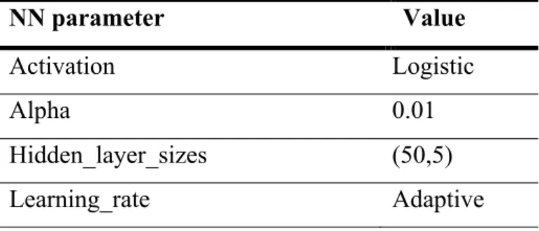
Table 2.6 – Optimized NN parameters by GridSearch

NN parameter Value Activation Logistic Alpha 0.01 Hidden_layer_sizes (50,5) Learning_rate Adaptive 2.3.6. Assumptions

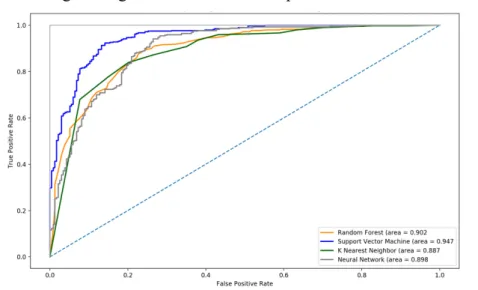
All tested algorithms’ parameters are optimized for this type of image data, concluding in a Receiver Operating Characteristic (ROC) curve plot. Repeatedly, this probability-based line is a plot of sensitivity as a function of the a-specificity (TPR AND TFR) (1 – specificity) where the total area underneath it (AUC) shows

25 a different algorithm score measure. The higher it reaches to 1, the better the quality of a tested algorithm. The ROC results for Random Forest, Support Vector Machine, K Nearest Neighbors and Neural Network with optimum parameters together with the corresponding AUC values are shown in Figure 2.17. These scores are based on image data generated with the InceptionResNetV2 CNN.

Figure 2.17 – Receiver Operating Characteristic Curves per algorithm

The AUC scores are in a range from 0.887 to 0.947 with the best predictions for the Support Vector Machine algorithm.

2.4. BINARY CNN COMPARISON

After optimizing the different hyperparameters, the algorithms are able to apply to the different CNNs to create an equal comparison. Each CNN experiment concludes with a ROC-curve together with time performance results. Besides the AUC, the complete confusion matrix will be considered in this experiment phase. The value of being able to predict the pneumonia cases correctly and minimize the false positive rate is the most important measure. The positive class refers to the fact that Pneumonia is diagnosed. The recall function is used as a second measure score where a value of 1 is perfect.

Combining these results lead to the best algorithm with pre-tested parameters per different CNN for the binary pneumonia prediction, whether or not pneumonia is observed. Paragraph 2.5 dives into the results for non-binary testing, given the same structure of steps. To obtain the best algorithm per CNN, the overall combined

26 subjective knowledge of scoring is used in these pre-experimental sections for preparing the significance testing in Chapter 4.

2.4.1. VGG16

The first CNN used to generate a classification model based on the pneumonia dataset is the VGG16. This feed forward network (Figure 2.18) is a relatively old CNN that enables converting an image to representing numbers.

Figure 2.18 – Architecture of VGG16 [92]

This convolutional- and Relu-process starts with increasing the depth with more than twenty times, followed up with a pooling resulting in a reduced three-dimensional size. After repeating this four times in a row, a matrix of 7 x 7 x 512 introduces the conversion to a fully connected network. Applying dense to the fully connected network results in a one-dimensional array which represents the input image.

This extracted data is used to test the capability of prediction as to whether or not an image contains pneumonia. The different algorithms with optimized hyperparameters are used for this optimization. Appendix 1 shows the ROC curve of the different algorithms. The AUC of the Neural Network scores the best, with a value of 0.947, but the time performance and recall are used as well in this experiment.

Appendix 4 shows that the Neural Network has the best possible score for the recall measure even though the follow-up algorithm (SVM) takes at least twice the time to generate a model. This means that there are no false negative predictions. It takes the algorithm approximately three minutes to generate predictions based on the

27 VGG16 output. The Neural Network will be used for future comparisons with the non-binary and SLM experiments.

2.4.2. VGG19

The evolved version of the VGG16 CNN is the expanded version which increases the number of weight layers by three, figured below. Introducing this extra sophistication creates a smoother way of reducing the size of image matrices.

Figure 2.19 – Architecture of VGG19 [100]

This extended version of the VGG CNN’s has the same pooling flow but the amount of layers between differ. The advantage of using a depth of nineteen convolution layers is the capability of identifying even more intricate patterns within the dataset. Besides the probability of gaining more insights into the image dataset, the disadvantage is the performance issues relating to its use.

Equally to the previous paragraph, the experiment is done for the different algorithms to assign the best to this particular CNN. The corresponding ROC curves and score table are shown in Figure 9.2 and Table 9.2. respectively, in Appendix 2. The best Area Under Curve score is generated for the Support Vector Machine: a score of 0.940.

The used time for generating a predictive model based on the VGG19 image output is more than 25 minutes, which is almost four times the performance time of the best VGG16 algorithm. The SVM recall has an almost perfect score, which shows that there is a low number of false negatives.

28 Compared with the VGG16 CNN, the improved version does not find a better AUC, recall or time performance measure. For this set of images, the VGG19 combined with the SVM finds a well-performing predictive model but not the best one.

2.4.3. InceptionV3

InceptionV3 (Figure 9.12, Appendix 12), developed based on GoogleNet architecture, is a CNN which is 48 layers deep and involves three softmax transformations to create multiple image extractions during the network. By implementing the Network in Network method [14] combined with sparsity in the layers, the purpose was gaining reduced computational resource gaining. This while improving the accuracy score.

Compared with the 16 and 19 layered VGG CNNs, Inception uses the capability of a parallel convoluted network. This complex method combined with lower parameterized blocks within it creates a wider perspective of understanding the images and the corresponding specific insights. Obviously, the shape of outputs differ between the different types of CNNs: The InceptionV3 uses meanwhile-exits ending with a softmax to flatten the output. The GoogleNet developers recognized the fact that it is not only the final layers that cover the discriminatory information. The intermediate features may describe the features differently and usefully for the end-description.

Appendix 3 contains the results after applying the different algorithms to the extracted-image dataset (extracted by InceptionV3 in 1110.50 seconds). The best scoring binary predictive model is the SVM in this experiment with an AUC of 0.939. The follow-up, Neural Network, has a better recall but the differences between these two are minimum. Both are acceptable as performing algorithm but the fact that the SVM is four times slower should be taken in account.

29

2.4.4. ResNet50

The fourth experimented CNN is the 50-layers deep Residual Network, which is developed for the use of residual learning. This architecture extracted from [100] consists of five different stages each with a residual block. All of them have three layers with 1x1 and 3x3 convolutions. The shortcuts between the blocks are called identity connections.

The change of residual learning is implemented to improve the learn-features method of multiple neural networks by calculating and optimizing using the residual. This residual can be understood as the subtraction of feature learned from input of that layer. Shortcutting the layers is a way to dive deeper but with the consideration of the previous-layer residuals. Taking the shortcuts into account the reduced information loss is introduced.

After extracting the image features, the described algorithms are used to predict whether or not a picture contains pneumonia. The scores are figured in a ROC curve and can be found in the table at Appendix 4. Determining the algorithm with the highest Area Under Curve is a competition between the Support Vector Machine and the Neural Network. Their AUC- and recall scores are respectively 0.953 and 1.0, and 0.954 and 0.995.

The differences between the two algorithms are minimal but a perfectly scoring recall is preferred. Even though the SVM performing time is twice the NN time based on this ResNet50 image extraction dataset.

2.4.5. InceptionResNetV2

The last tested pretrained network is the combination of the previous two CNNs: InceptionV3 and ResNet50, which logically concludes in a combined architecture

30 shown in APPENDIX 13. This architecture is too complicated to show completely in this chapter, but the main structure is based on a combination of two previous described CNNs.

Uses the residuals and complex network in network method based on ResNet and the intermediate feature extraction from InceptionV3. The shortcut method is implemented between the blocks to reduce information loss based on residuals. Furthermore, waste of information will be reduced through the possibility of selecting a “halfway” feature extraction or insight. Both advantages lead to a more sophisticated CNN but would make it harder to understand and the network needs more time to proceed a well performing model. The 1871 seconds it takes to extract features from the image dataset illustrates the complexity of this algorithm. This CNN needs relatively more time to result in a score that is not better than the previous experiments.

The SVM is the best scoring (AUC of 0.947) predictive algorithm based on the InceptionResNetV2 extracted features. A corresponding recall of 0.997 shows that the model almost perfectly predicts whether or not an image contains Pneumonia. This value explains the fact that there is a very small number of false negatives: predicted as non-pneumonia, but actually involves pneumonia. The disadvantage of the SVM is the slow performing time; approximately 17 minutes.

2.4.6. Binary summarized

The different models created based on the pneumonia dataset are listed in table X. Five CNNs are tested with the several tested algorithms, all set with the optimized hyperparameters. The combination of all best performing CNN and algorithm are listed with the corresponding score measures. The best performing binary prediction model is the combination of ResNet50 and Support Vector Machine with a perfectly scoring recall and an AUC of 0.953. It takes the longest time to perform this model, more than 70 minutes, but it is worth it.

31 Table 2.7 – Binary CNN results summary

CNN/algorithm Performance CNN (s) /algorithm (s) AUC Recall VGG16 - NN 1295 - 178 0.947 1.0 VGG19 - SVM 1509 - 685 0.940 0.997 InceptionV3 - SVM 1111 - 2121 0.939 0.987 ResNet50 - SVM 1449 - 2840 0.953 1.0 InceptionResNetV2 - SVM 1871 - 1070 0.947 0.997 2.5. NON-BINARY CNNS

After predicting whether an image contains pneumonia or not, the type of pneumonia is then decided. The Pneumonia cases are divided into bacterial and viral, which creates a three-class dataset.

Experimenting with these different classes requires a one-versus-all method: Each target will be tested against the remaining two classes. This method is comparable with the binary prediction in the previous chapter, but then applied to each target value. Applying this for each algorithm per CNN creates three different ROC-curves and corresponding AUC values. A more accurate way to conclude the scores per experiment is to average the three ROC-curves but keeping the AUC’s. This average is calculated with the micro average method:

!o/

pppppp_{qQrst =} ∑ 68< ∑ ;8<

A transformation from three classes as target value to a binary notation is necessary to apply the one-versus-many method. Each experiment uses the pre-optimized hyperparameters per algorithm and shows besides the average ROC-curve and AUCs the recall value and time required to perform the model based on the CNN features. The 0, 1 and 2 describe respectively no-, bacterial- and viral infection.

32

2.5.1. VGG16

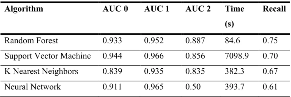
The first tested CNN is the VGG16 but with the non-binary targets, known as not infected, bacterial infection and viral infection. The one-versus-many method results in various AUC values, shown in Table 2.8. Besides the AUC, the time and recall scores are listed per experimented algorithm. Appendix 6 contains the corresponding !o/pppppp value and curve per algorithm to create more nuanced insights about the performance.

Table 2.8 – Non-binary VGG16 results

Algorithm AUC 0 AUC 1 AUC 2 Time (s)

Recall

Random Forest 0.933 0.952 0.887 84.6 0.75

Support Vector Machine 0.944 0.966 0.856 7098.9 0.70 K Nearest Neighbors 0.839 0.935 0.835 382.3 0.67

Neural Network 0.911 0.965 0.50 393.7 0.61

Remarkable is the higher performance time of the SVM without obtaining the best recall or !o/pppppp score. Moreover, the implemented Neural Network is not

sophisticated enough to predict the three target values equally. Even though the model contains more than two output neurons and a “softmax” function to

determine probabilities, it seems complicated to distinguish the VGG16 extracted features non-binary.

The Random Forest has the highest micro-averaged AUC value and the best recall-score while performing faster than the other three algorithms based on the in 1605 seconds extracted VGG16 features.

2.5.2. VGG19

VGG19 is the next tested CNN under the same circumstances. This expanded VGG version takes 5 minutes longer to extract the non-binary dataset than the one of the previous experiment. Table 2.9 contains the results of the tests per different algorithm and the corresponding micro-averaged curves are shown in Appendix 7.

33 Table 2.9 – Non-binary VGG19 results

Algorithm AUC 0 AUC 1 AUC 2 Time (s)

Recall

Random Forest 0.937 0.963 0.899 87.7 0.77

Support Vector Machine 0.940 0.962 0.832 6919.5 0.68 K Nearest Neighbors 0.856 0.948 0.844 382.0 0.7

Neural Network 0.628 0.973 0.872 220.9 0.67

Increasing the layers of the CNN network could not solve the disability of the Neural Network to create a well-scoring one-versus-many AUC. In this case it seems like the Neural Network lost its knowledge of how to determine whether or not an image contains any type of pneumonia. Concludingly this type of NN is not capable enough to distinguish multiple target values equally. A score of 0.628 is improved compared with the previous results, but still not better than the other algorithms.

The RF is again the winner of this experiment, with a recall of 0.77 and a !o/pppppp of 0.885, having slightly improved compared with the previous VGG version. The SVM shows its struggles gaining information of multiple classes again by performing an notably long time.

2.5.3. InceptionV3

The third experiment of this non-binary section is the testing of the algorithms based on the 1070 seconds long InceptionV3 extracted features. The results of this test are listed in Table 2.10 and the curves are shown in Appendix 8.

Table 2.10 – Non-binary InceptionV3 results

Algorithm AUC 0 AUC 1 AUC 2 Time (s)

Recall

Random Forest 0.907 0.929 0.874 303.2 0.67

Support Vector Machine 0.939 0.939 0.855 15171.6 0.72 K Nearest Neighbors 0.918 0.930 0.855 782.3 0.76

34 A new algorithm performs best: The K-Nearest-Neighbors algorithm. This

algorithm has the highest !o/pppppp value without scoring the highest AUC per different one-versus-many method. Additionally, the recall score of 0.76 is the runner-up after NN. Knowing that the NN could not predict the 2-versus-(0 and 1) accurately, namely a score of 0.567, the runner-up recall score is assumable in this case. For non-binary prediction this is still a lower recall score than the binary results, where there were minimal false negative predictions.

2.5.4. ResNet50

The 50-layers deep CNN is the next network of this experimental phase. For the binary test of algorithms this type of feature extraction was the one with the longest performing time of algorithms, which could possibly lead to a similar effect for the non-binary cases. The results of this experiment are listed in Table 2.11 with the ROC curves attached in Appendix 9.

Table 2.11 – Non-binary ResNet50 results

Algorithm AUC 0 AUC 1 AUC 2 Time (s)

Recall

Random Forest 0.940 0.956 0.893 232.2 0.77

Support Vector Machine 0.953 0.972 0.886 29839.7 0.74 K Nearest Neighbors 0.896 0.961 0.865 1554.8 0.75

Neural Network 0.887 0.963 0.871 3401.1 0.71

The Neural Network was able to create a well performing prediction of classes in all three cases. This means that this CNN creates an output which could be used as a NN input. Nevertheless, the ROC curve plot in Appendix 9 shows a non-fluently shaped curve, as noted in previous results. This could be caused by the micro-average method. Appendix 10 includes a plot of the three one-versus-many cases and aids in justifying this expectation. Assumed is that averaging the false-positive- and true-positive rates introduces odd shaped curves, but still represents all three parts of the method.

Although the NN was able to distinguish between the different classes, it could not compete against the fast-performing Random Forest with a recall of 0.77,

35 produces a predictive model scoring a !o/pppppp of 0.891. This means that the RF is the best performing algorithm based on this 1597 second during feature

extraction.

2.5.5. InceptionResNetV2

The last tested CNN is the longest performing binary network, but with its

1502 seconds it has the second place of performing time in the non-binary CNN feature extractions. The tested algorithms are listed below in Table 2.12 and the corresponding ROC-curves with calculated !o/pppppp are shown in Appendix 11.

Table 2.12 – Non-binary InceptionResNetV2 results

Algorithm AUC 0 AUC 1 AUC 2 Time (s)

Recall

Random Forest 0.896 0.937 0.879 230.3 0.72

Support Vector Machine 0.947 0.957 0.865 10559.7 0.73 K Nearest Neighbors 0.887 0.936 0.862 582.4 0.75

Neural Network 0.420 0.946 0.597 269.7 0.68

After taking a long time to extract the image features, the NN could not create a useful distinction between the three classes, providing two bad-scoring AUCs out of three different one-versus-many tests. The best matching curve with highest !o/pppppp attached is measured for the K Nearest Neighbor algorithm. With an !o/pppppp of 0.870 and the highest recall, 0.75, this is the best performing algorithm based on the InceptionResNetV2 extracted features. With an approximately twenty times faster performing time compared with the SVM, the KNN would be used combined with this CNN.

2.5.6. Non-binary summarized

The five best performing CNN and algorithm combinations are listed in Table 2.13 which exists of Random Forests and K Nearest Neighbors algorithms. All of them with an !o/pppppp scoring in a range between 0.870 and 0.981. The best performing combination is the ResNet50 with a RF in this experiment. A recall of 0.77 still

36 requires some improvement, while some Pneumonia cases would not be recognized.

Table 2.13 – Non-binary results summary

CNN/algorithm Performance CNN (s) /algorithm (s) vwx pppppp Recall VGG16 – RF 1150 - 84.6 0.874 0.75 VGG19 – RF 1490 - 87.7 0.885 0.77 InceptionV3 - KNN 1070 - 782.3 0.886 0.76 ResNet50 - RF 1597 - 232.2 0.891 0.77 InceptionResNetV2 - KNN 1502 - 582.4 0.870 0.75 2.6. CONCLUSION

Considering Table 2.7 and Table 2.13 of previous sections, there is a major difference between the quality and models of binary and non-binary testing. The binary experiments lead to significantly better scores for !o/pppppp and recall, with time consuming algorithms when compared with the non-binary ones.

There are CNN and algorithm combinations which determine multiple classes for the extracted image features, however this could be enhanced by increasing the ability of insights creation by expanding the train and test data sets. Currently it settles for RF and KNN, but the Neural Network could possibly create more valuable knowledge with a bigger number of data observations.

The ResNet50 is the best performing CNN for binary and non-binary, but respectively SVM and RF create the difference. Competing this against the Semantic Learning Machine creates the possible need of a Genetic Algorithm in this kind of multi-class image prediction.

37

3. SEMANTIC LEARNING MACHINE ALGORITHM

This chapter contains a description of the Stochastic Neural Network construction called Semantic Learning Machine followed by a binary and non-binary experiment as done in previous chapter. Comparing the results with the previously tested algorithms creates knowledge about the ability of multi-class prediction based on various CNN extracted features.

3.1. EXPLAINED

The Semantic Learning Machine (SLM) is a stochastic Neural Network construction algorithm originally derived from Geometric Semantic Genetic Programming (GSGP). The fact it searches over unimodal landscapes is probably the most promising characteristic [10]. It uses the error as a measurement of the distance to the known targets. Previous research show that it has the capability of outperforming various prediction algorithms such as the common backpropagation based NN. The SLM method implies that there are no local optima; just one single local optimum which is ideally reached through the unimodal landscape. The SLM method can be compared with a Hill Climbing algorithm without accepting local optima [9].

SLM uses an application of multiple non-fixed-topology NNs and minimizes the error of distance by mutating during the evolution, which introduces some parameters and properties of the SLM. Evolutionary algorithms use iterations and population sizes to preserve the model’s searching space from infinity.

The question of matter in this research is if it outperforms other algorithms based on the Pneumonia extracted image features.

3.2. METHODOLOGY

An intensive research and engineering of SLM implemented by Jagusch, J.B. [10] is used as the base of this chapter’s experiments. The binary test required some additions regarding the output vectors for this specific comparison with previously tested algorithms. The adjustments to use the SLM for non-binary perspectives are mainly extended by Gonçalves, I. and Castelli, M.

38 Specialisation inside the SLM is possible by setting the learning step as fixed (FLS) or optimized (OLS). The SLM-OLS method will be used for both binary and non-binary experiments, while the question is if the SLM outperforms the other algorithms. Resampling the dataset into ten random sampled datasets is used to reduce the possible overfitting after iterating a while. The setup of these experiments is based on the setup of Vanneschi et al. [26] and Gonçalves et al [8]. A number of iterations is used in this research differs to this research, using 200 iterations/generations. Population/sample size is set to 100 and the training-testing division is set to 70-30, which is commonly used in predictive models.

3.3. EXPERIMENTS

Running these experiments to compare the different CNNs used as a source of the SLM is explained in this section. For binary and non-binary testing the Root Mean Squared Error (RMSE) will be used for the proof of significance. Moreover, the recall, performance time and AUC value will be used averaged over the number of runs done per CNN for general performance insights.

3.3.1. Binary

This experiment contains a SLM set with the previous mentioned assumptions for each of the CNN extracted image features: VGG16, VGG19, InceptionV3, ResNet50, InceptionResNetV2. The RMSE per CNN is presented as a boxplot in Figure 3.1. This boxplot is based on 10 runs per CNN, which means that each boxplot is based on 10 RMSE values. The dark lines in the middle show the average of the runs with half of the observations included in the complete box.

39 The ResNet50 CNN seems to introduce the best performing SLM application, the corresponding insight measures are listed in Table 3.1. The InceptionResNetV2 method creates the least spread between the RMSE’s against a VGG19 with a large box; middle half of the observations. The complete table is generated by averaging each measure over 10 SLM runs.

Table 3.1 – Binary SLM results

CNN RMSE Recall AUC Time (s)

VGG16 0.378 0.501 0.832 192.8

VGG19 0.306 0.875 0.974 258.0

InceptionV3 0.320 0.805 0.946 346.4

ResNet50 0.289 0.813 0.958 502.1

InceptionResNetV2 0.301 0.827 0.958 358.2

The VGG16 CNN scores the worst for each prediction quality measurement. With a slight change from 16 to 19 layers, it seems to improve within the VGG’s. The ResNet50 CNN with its lowest RMSE, does not have the highest average scores for the recall and AUC measures but the significance will be shown in the next chapter with its p-value compared with the common algorithms of Chapter 2.

3.3.2. Non-binary

Secondly, the SLM is tested for binary purposes. This compared with the non-binary results of Chapter 2 shows the capability of this algorithm of predicting multiple classes. A maximum number iteration of 50 is used to prevent local CPU performance issues. Figure 3.2 illustrates the distribution of the RMSE per CNN applied to the SLM in a boxplot graph.