Nova School of Business and Economics
The Effect of Basel III
on Earnings
Management using
Loan Loss Provisions
A project carried out on the International Master in
Management under the supervision of Xanthi Gkougkousi
Iselin Rosvold – Student Number 2841
26.05.2017
1 Content 1.0 Introduction ... 2 2.0 Theory ... 3 2.1 Basel Accords ... 3 2.2 Earnings Management ... 6
2.3 Loan Loss Provisions as a Tool for EM ... 7
2.4 Accounting Regulation ... 8
3.0 Previous Research on Basel Accords’ effect on EM using LLPs ... 8
4.0 Hypothesis Development ... 9
4.1 Research Question ... 9
4.2. Hypothesis ... 11
5.0 Methodology ... 13
5.1 Data Sample ... 13
5.2 Dependent and Independent Variables ... 13
5.3 Outliers ... 17
5.3 Descriptive Statistics ... 18
5.5 Regression Analysis ... 19
Estimation Methods ... 19
Breusch-Pagan Lagrange multiplier (LM) ... 19
Hausman Test ... 19
5.6 Regression Diagnostics ... 20
Heteroscedasticity ... 20
Autocorrelation ... 20
Multicollinearity ... 20
Checking Normality of Residuals ... 20
6.0 Analysis and Result Discussion ... 21
6.1 EBTP-Model ... 21
6.2 Basel III-Model ... 24
7.0 Conclusions, limitations and further research ... 25
2
The Effect of Basel III on Earnings Management
using Loan Loss Provisions
ABSTRACT
In this paper, I look at the effect of the implementation of Basel III on the practice of earnings smoothing using loan loss provisions in listed European banks. The aim is to contribute to a better understanding of how international regulation influence discretionary behavior, as well as
considering if the Basel enhancements reduce aggressive income smoothing, as the activity can lead to consequences contrary to the regulation’s objectives. My main findings were statistically
insignificant, however it indicated an effect of a reduced earnings smoothing activity using loan loss provisions in the three years after Basel III was implemented.
Key words: Earnings management, international regulation, loan loss provisions, European banks
1.0 Introduction
The third Basel Accord was implemented in 2011 to improve stability and soundness of individual banks and the global financial system. It was the international regulatory government’s answer to the loophole in financial standards and regulation which became evident under the financial crisis in 2007/2008. The objectives of this new capital accord include improving management of credit, market and operational risks. In this research, I will look at the effect the implementation of this Basel Accord has on the practice of earnings management, more specific earnings smoothing using loan loss provisions in European banks. It will be beneficial to know if there is a more aggressive earnings smoothing activity correlated with the implementation of Basel III, as it can have
3 unintended consequences on the objectives of the Basel Accord, and further oppose the purpose it. Discretionary provisioning of loan loss reserves can reduce banks’ transparency and hinder supervision by regulators (Finch 2009; Bushman and Williams 2012), it can be pro-cyclical (Skala 2015) which further can increase market risk globally for banks (Basel Committee On Banking Supervision 2011), furthermore it may lead to higher operational risk for banks on an individual level (Basel Committee on Banking Supervision 2015), and it gives managers a trade-off dilemma of either having a solid capital reserve or stabile earnings. This trade-off can result in higher credit risk when the managerial decision is to smooth earnings.
The majority of earnings management studies show that income smoothing practices using loan loss provisions, has been present in many financial institutions for decades (Leventis, Dimitropoulos, and Anandarajan 2011; Anandarajan, Hasan, and McCarthy 2007; Curcio and Hasan 2015; among others), and are derived from many different incentives. According to Ozili (2017), there do exist research on earnings management’s effect of the implementation of the first and second Basel Accord, but limited, if not none, on the third accord.
This paper’s structure starts with a presentation of relevant fundamental theory, followed by the research question, its relevance, and the hypothesis. I will briefly present previous research on the topic of earnings management under the Basel regulations. Further, I explain the method used in the research, before I go through the analysis and results, and discuss the interpretation of these. The paper ends with a conclusion including the study’s limitations and suggested further research.
2.0 Theory
2.1 Basel Accords
The Basel Accords are three sets of banking capital regulations (Basel I, II and III) set by the international supervisory authority, Basel Committee on Bank Supervision (BCBS). The first
4 accord was created in 1988, with the intent to mitigate the credit risk in banks on an international level. An essential reason for this agreement was the frequent bank failures during the 1980s. The fact that countries’ external indebtedness was growing unsustainably, created a need for credit risk management by increasing capital requirements for financial institutions (Zaher 2007).
The minimum capital requirement was set to be a capital adequacy ratio1 of 8% (Basel Committee on Banking Supervision 2015).The Basel Accord also divided the capital in two tiers, where Tier 1 is the core capital generated to support when banks absorb unexpected losses, and Tier 2 includes hybrid instruments and capital reserves, which is less reliable to cover losses. As the world’s capital markets evolved, there was a need for enhancements in the Basel Accord, and in 2008 Basel II was implemented. After the financial crisis in 2007-2008, there was a common consensus that the need for an even more enhanced supervisory accord was present. Consequently, Basel III was already implemented in 2011.
BASEL III
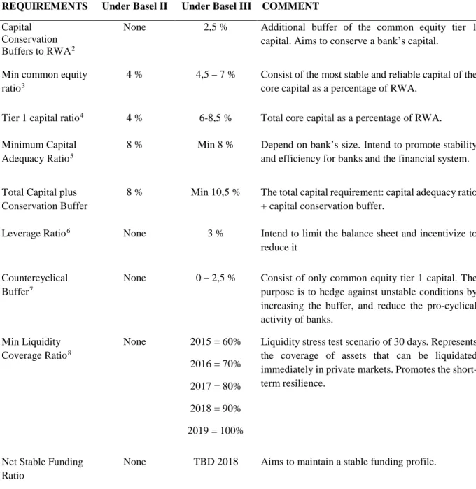
Basel III brings focus to greater resilience at the individual bank level, with the aim to reduce risk of a system-wide unhealthy economic development, such as the case of the subprime-crisis. This accord mitigates not just credit risk, but also market and operational risk. The purpose of the third accord is to improve banks’ ability to absorb losses and shocks, improve risk management and governance, and strengthen their transparency and disclosures. The changes from the second to the third Basel Accord is summarized in table 1 below. As the improvements are extensive and comprehensive, some of the requirements are implemented by a phase in-period. I will elaborate on the implications of the Basel III’s enhancements in the hypothesis discussion in section four.
1 The capital adequacy ratio is the total capital over risk weighted assets (RWA). RWA is the value of the bank’s assets
5
Table 1: Changes in the requirements from Basel II to Basel III
REQUIREMENTS Under Basel II Under Basel III COMMENT
Capital Conservation Buffers to RWA2
None 2,5 % Additional buffer of the common equity tier 1 capital. Aims to conserve a bank’s capital.
Min common equity ratio3
4 % 4,5 – 7 % Consist of the most stable and reliable capital of the core capital as a percentage of RWA.
Tier 1 capital ratio4 4 % 6-8,5 % Total core capital as a percentage of RWA.
Minimum Capital Adequacy Ratio5
8 % Min 8 % Depend on bank’s size. Intend to promote stability and efficiency for banks and the financial system.
Total Capital plus Conservation Buffer
8 % Min 10,5 % The total capital requirement: capital adequacy ratio + capital conservation buffer.
Leverage Ratio6 None 3 % Intend to limit the balance sheet and incentivize to
reduce it
Countercyclical Buffer7
None 0 – 2,5 % Consist of only common equity tier 1 capital. The purpose is to hedge against unstable conditions by increasing the buffer, and reduce the pro-cyclical activity of banks. Min Liquidity Coverage Ratio8 None 2015 = 60% 2016 = 70% 2017 = 80% 2018 = 90% 2019 = 100%
Liquidity stress test scenario of 30 days. Represents the coverage of assets that can be liquidated immediately in private markets. Promotes the short-term resilience.
Net Stable Funding Ratio
None TBD 2018 Aims to maintain a stable funding profile.
References: (Basel Committee On Banking Supervision 2011; Basel Committee on Banking Supervision 2015; Basel Committee on Banking Supervision 2014; Basel Committee on Banking Supervision 2013)
2 Additional buffer of common equity tier 1 capital to risk-weighted assets 3 Calculated: Tier 1 common equity to risk-weighted assets
4 Calculated: Total tier 1 capital to risk-weighted assets
5 Calculated: Total capital (Tier 1 + Tier 2) to risk-weighted assets
6 Computed as tier 1 capital to the total of on- and off-balance assets, less intangible assets 7 An additional buffer which increase in unstable financial times. Represents percentage of RWA. 8 Computed as the percentage of total high-quality liquid assets
6 2.2 Earnings Management
Earnings management (EM) is the practice of managers using their own judgement when structuring transactions and financial reports with the intent to control the outcome of earnings (Healy and Wahlen 1999). In this thesis, I will look at the legal practice of EM, which is the managerial judgement of reporting numbers within the boundaries of reporting standards. When conducting EM, managers either maximize or minimize income, or they smooth the income. Bank income smoothing is the process in which banks make reported earnings appear stable over time so that reported earnings never seem to be too high or too low (Ozili 2017a). There exist two types of legal earnings management (1) real actions, which involves managing working capital, and (2) accounting policy choice, which includes deciding on accounting policies and use of discretionary accruals. The latter allow you to some degree decide on the valuation of certain accruals, within the mentioned boundaries of the reporting standards. The use of discretionary accruals to smooth earnings is the part of EM that I will focus on in this paper. As I state in the intro, I will focus on the use of loan loss provisioning (LLP) for the practice of income smoothing.
LLPs may also be used for signaling and capital management (Greenawalt and Sinkey 1988). Though the latter is closely related to the Basel Accord, I limit my research to income smoothing. The practice can be beneficial in terms of saving for a rainy day (Greenawalt and Sinkey 1988), protecting banking jobs (Defond and Park 1997; Fudenberg and Tirole 1995), reduce information asymmetry between owners and managers (Tucker and Zarowin 2006), and improving bank stability by smoothing out abnormal fluctuations in reported earnings (Wall, L. D. and Koch 2000). However, EM can also influence regulatory effects and distort the disclosure of true information, and further reduce the usefulness of financial information to decision makers. In addition, income smoothing may be considered unethical if the managers opportunistically receive bonuses (Healy
7 and Wahlen 1999), reduce the informativeness of reported earnings (Leventis, Dimitropoulos, and Anandarajan 2011; Tucker and Zarowin 2006), or lower the quality of reported earnings (Ahmed, Neel, and Wang 2013). According to Andrews et al. (2010), the banks engage in EM using LLPs for several reasons depending on their business objectives, governance, and performance. Here, the volatility level of earnings plays an essential role.
2.3 Loan Loss Provisions as a Tool for EM
“Bank lending to borrowers gives rise to credit risk where borrowers are unable to repay the principle and/or interest on loan due to unfavorable economic conditions and related factors. To mitigate credit risk, in principle, banks will set aside a specific amount as a cushion to absorb expected loss on banks’ loan portfolio and this amount is referred to as loan loss provisions (LLPs) or provisions for bad debts; therefore, loan loss provisions estimate is a credit risk management tool used by banks to mitigate expected losses on bank loan portfolio” (Ozili 2017a).
As stated earlier, LLPs are a discretionary accrual, which implies managerial judgement on its size. During the last decades, there have existed a growing concern that the objectives behind the LLP activity are not solely driven by credit risk, but rather opportunistic financial reporting incentives (Healy and Wahlen 1999; Gombola, Yueh-fang Ho, and Huang 2016). Several previous researches have proven that LLPs are used as a tool to manage earnings (Fonseca and González 2008; Leventis, Dimitropoulos, and Anandarajan 2011; Anandarajan, Hasan, and McCarthy 2007; Collins, Shackelford, and Wahlen 1995; among others). However, there are also researchers who did not find evidence for earnings management using LLPs (Ahmed, Takeda, and Thomas 1999). The unique feature of this accrual, and probably the reason why it is widely used in EM, is that changes in LLPs simultaneously influence the bank’s profitability and risk (Bushman and Williams 2012). This creates a trade-off where increased LLPs gives lower earnings, but a higher buffer
8 against expected absorbed losses. While decreased LLPs, result in higher earnings, but it also a higher risk that the bank’s total loan loss reserves do not cover expected losses9.
2.4 Accounting Regulation
In 2005, the first form of international accounting policy was implemented, the international financial reporting standards (IFRS). In 2015, more than 100 countries had implemented IFRS as mandatory practice for listed companies. Today however, there are still many companies using the specific country’s general accepted accounting policies (GAAP), including listed companies in the Unites States. Accounting standards are an essential determinant of banks’ behavior (Basel Committee On Banking Supervision 2011). According to Leventis et al. (2011), the practice of EM using LLPs was significantly different after the implementation of IFRS. Consequently, I will focus on European listed banks reporting under IFRS to make sure that all firms in the sample operate under similar regulatory requirements and use the same accounting standards.
3.0 Previous Research on Basel Accords’ effect on EM using LLPs
There does exist some research on how the three Basel Accords affect the banks’ use of LLPs for earnings management. With the implementation of the first accord, there has been found evidence for a more aggressive earnings management activity (Collins, Shackelford, and Wahlen 1995; Anandarajan, Hasan, and McCarthy 2007). Researchers argue that this probably is because the first accord had an incentive to engage in more aggressive EM because of the loophole that LLP was limited to only 1.25% in the capital adequacy ratio. This implies that changes in LLP would not
9 Increasing LLPs with €1 increases LLRs with €1 but reduces earnings with €1-(€1*tax rate). This implies that
capital increases with €1*tax rate (Collins, Shackelford, and Wahlen 1995). Decreasing LLPs with €1 reduces LLRs with €1 and increases earnings with €1-(€1*tax rate). Capital than reduces with €1*tax rate (Collins, Shackelford, and Wahlen 1995).
9 affect the regulatory capital if the total loan loss reserves exceeded 1,25%. However, Ahmed et al. (1999) did not find any evidence for this activity in the same period. One of the objectives of the second accord, was to reduce the discretionary judgement possibilities for banks. This was done by requiring the banks to separate their loans into categories according to the probability of default (Basel Committee on Banking Supervision 2015). As a result, researchers found indications for a decreased earnings management activity, but it was still present (Spitteler 2011).
More recent studies prove that banks also engage in earnings smoothing with LLPs after the implementation of the third Basel Accord (Stoian and Norden 2013; Magnis and Iatridis 2017). Gombola, Yueh-fang Ho, and Huang (2016) find that the earnings management activity post Basel III, is positively related to leverage and negatively related to liquidity, which are two factors that got stricter regulated in the Basel III accord. Research by Ozili (2017b), shows that the discretionary provisioning among Western European banks in the post-crisis period is driven by both credit risk and income smoothing considerations. However, none of these new research papers test for a difference in the EM activity before and after the implementation of the third Basel Accord. Furthermore, by focusing on this difference, this research’s findings can contribute to the income smoothing literature, as well as providing an additional perspective for regulators to see if the third Basel Accord is pursuing its purpose, which is a concern I will discuss in the next section.
4.0 Hypothesis Development
4.1 Research Question
How does the implementation of the third Basel Capital Accord effect the activity of earnings management using LLPs to smooth income in European banks?
10 As already mentioned, several studies from the last decades have found conclusive evidence that earnings management practices using LLPs are common in financial institutions across the world (Greenawalt and Sinkey 1988; Wahlen, 1994; Leventis et al 2011; among others), and some studies did not find sufficient evidence for this (Ahmed, Takeda, and Thomas 1999), but as I already stated, there is not yet done research on Basel III’s effect on the aggressiveness of EM activity.
As the banking sector has the mandate to lend money to their communities, they play a key role in the national and global economies (Lobo 2016). Because of their given importance, their estimates on LLP, which affect the stability and soundness of the bank, will further influence national and global capital markets by changes in this function. This is also one of the reasons why LLPs have become one of the most debated accounting number in financial reporting of banks since the global financial crisis (Ozili 2017a). It is in this post-crisis period that the third Basel Capital Accord has been implemented. For this reason, in addition to the alterations made from the second accord, it will be interesting to see if there exist any differences in income smoothing practices pre-and post-Basel III. Several previous studies include models with provisioning incentives of capital management, and proven this to be a natural activity to conduct when there are changes in the international regulatory capital requirements (Anandarajan, Hasan, and McCarthy 2007; Ahmed, Takeda, and Thomas 1999; Curcio and Hasan 2015; Collins, Shackelford, and Wahlen 1995). Consequently, I exclude this focus in my research question.
My choice to examine the combination of income smoothing with LLPs and the implementation of Basel III, is based on the implications that this EM activity can have on the capital accord’s purpose and objectives. There are four ways the activity can affect these. First, we have the issue that EM using LLPs can reduce the degree of transparency in the financial reports. Judging the size of LLPs based on earnings volatility, rather than credit risk, may not reflect the underlying
11 economic reality (Ozili 2017a), which effect the objective of strengthening transparency and disclosure. A second issue is that the activity can affect the financial stability by being pro-cyclical (Basel Committee On Banking Supervision 2011), which interfere with the intended consequences of introducing a countercyclical buffer. The same effect can also arise as EM using LLPs have the effect of making provisioning out of time, because of the influencing factor of cyclicality. According to Laeven and Majnoni (2003), delays in loss provisioning have been found to contribute to reducing lending activities, as the delay will put pressure on the bank to increase provisions even more exactly in the part of the cycle where capital requirements are most binding, and this will further affect the financial stability.
Third, it is found that banks conducting provisioning designed for earnings smoothing, will have higher operational risk, than the banks that perform provisioning based on anticipated future loan losses (Basel Committee on Banking Supervision 2015). This takes us to the final issue, which is the mentioned trade-off between having solid loan loss reserves, which mitigate the operational risk, or smooth earnings. As we see from the reasons above, this research will be beneficial from a regulatory perspective, to better understand needed enhancements which can mitigate unintended effects if this is found. In addition, it can contribute to the earnings management theory, because of the mentioned lack of research done in this area combined with the implementation of Basel III. 4.2. Hypothesis
H0: Basel III will have no effect on banks’ earnings smoothing activity.
HA: Earnings smoothing activity is less aggressive in the years after the implementation of the
12 As I discussed in the third section, earlier studies have found evidence for both increasing and decreasing effects in EM activity related to changes in the regulations of the first and second Basel Accords. Other previous studies show that stricter supervision of banks reduce the extent of bank income smoothing (Leventis, Dimitropoulos, and Anandarajan 2011; Cavallo and Majnoni 2001; Oosterbosch 2010; Duru and Tsitinidis 2013). The changes from Basel II to Basel III make the requirements regarding discretionary accruals stricter. Consequently, I believe it will reduce the activity of income smoothing among the banks that operates under this new Basel Accord.
To be more specific, there are four distinct regulatory enhancements from Basel II to Basel III that I base my hypothesis upon. (1) Because the enhancements include a significant increase in the capital adequacy ratio, there will most likely be an increase in LLP related to the need to meet the minimum capital requirements. As I discussed earlier, this is a natural consequence of changes in regulatory capital. As capital management has proven to have a negative correlation with LLP, this need to increase capital can reduce the respective year’s part of provisioning in which can be discretionary evaluated for smoothing purposes. In other words, it can hinder the management to increase earnings via LLPs if the provisioning is already altered for capital management incentives; (2) Studies show that income smoothing is negatively related with liquidity and bank leverage (Gombola, Yueh-fang Ho, and Huang 2016). The new Basel Accord’s requirements include high liquidity and leverage ratios which are presented in table 1. This implies that the implementation of these ratios will decrease the smoothing activity; (3) The stricter disclosure requirements in Basel III, can reduce EM as this has been proven before when banking supervision gets stricter (Cavallo and Majnoni 2001), or with higher audit quality (Kanagaretnam, Lobo, and Mathieu 2004); (4) Studies show a strong positive relation between EM and risk-taking, which indicates that risk-taking is a factor that can lead to earnings volatility (Andrews et al. 2010). As a result of
13 the mentioned enhancements in the accord, the banks will have a lower risk profile, and further, the bank’s earnings will naturally become smoother over time. This eliminates the need for conducting earnings smoothing (Andrews et al. 2010).
5.0 Methodology
5.1 Data Sample
To test the H0, I will use a sample of 75 European banks from 22 different countries, see appendix
3 for more comprehensive information about the sample. The financial data is panel data from the Basel II period of 2008-2010 (pre-Basel3) and Basel III period of 2011-2013 (post-Basel3). All banks are listed, and therefore, as mentioned, are reporting under IFRS. The total of observed years is 418, where 205 are pre-Basel3 and 213 are post-Basel3. All financial data is collected from Bloomberg Database, while data concerning GDPs is collected from World Economic Outlook Database, edition April 2016 (International Monetary Fund 2017).
The disadvantage with panel data is that it is more complex than purely cross-sectional or time series data. The most important drawback is the difficulty in designing the sample scheme to reduce the problem of subjects leaving the study prior to its completion, also known as attrition (Frees 2004). This have reduced the sample size from 636 to 418 observations, but in turn increased the validity of the study. In this process, I have limited the sample to listed commercial banks and excluded all in which are unlisted or private.
5.2 Dependent and Independent Variables
To detect earnings smoothing using LLPs, I will look at the relationship between the respective year’s LLPs and earnings before provisions and taxations. I will use a modified version of the regression model that Ahmed et al. (1999) use to examine the effect of Basel I on earnings and
14 capital management, where I exclude independent variables that are not relevant and add a few control variables which I find relevant for the research’s purpose and specific period. They are also in line with what Fonseca and González (2008) state that the banks’ income smoothing depends on; regulatory supervision, financial structure and financial development. The basic model is also used in more recent research on earnings management by, among others, Anandarajan et al. (2003, 2007) and Leventis et al. (2011). The model is based on the accrual monitory model developed by Jones (1991) which is proven to be the most accurate model for detecting earnings management (Dechow, Sloan, and Sweeney 1995). Hence, I will use the following model:
𝐿𝐿𝐿𝐿𝐿𝐿 = 𝛽𝛽0+ 𝛽𝛽1 𝐸𝐸𝐸𝐸𝐸𝐸𝐿𝐿 + 𝛽𝛽2 𝐸𝐸𝐸𝐸𝐸𝐸𝐿𝐿 ∗ 𝐸𝐸𝐵𝐵𝐵𝐵 + 𝛽𝛽3 ∆𝐺𝐺𝐺𝐺𝐿𝐿 + 𝛽𝛽4 ∆𝑁𝑁𝐿𝐿𝐿𝐿 + 𝛽𝛽5 𝑁𝑁𝑁𝑁𝑁𝑁 + 𝛽𝛽6∆𝐿𝐿𝐿𝐿𝐿𝐿𝐿𝐿𝐿𝐿
+ 𝛽𝛽7𝑁𝑁𝑁𝑁𝑁𝑁 + 𝛽𝛽8𝐸𝐸𝐵𝐵𝐵𝐵 𝛽𝛽9 𝑁𝑁𝑁𝑁𝐶𝐶𝐵𝐵𝐶𝐶𝐵𝐵 + 𝑒𝑒
where:
LLP Loan loss provisions to average loans outstanding
EBTP Ratio of earnings before taxes and provisioning to average total assets
EBTP*BAS Interaction of EBTP with Basel III
ΔGDP Change in gross domestic product
ΔNPL Change in non-performing loans to average loans outstanding
NCR Ratio of net commission revenue to total assets
ΔLoans Changes in outstanding loans
NCO Net charge offs to average loans outstanding
BAS Dummy variable: (0) = pre-Basel3 (1) = post-Basel3
CRISIS Dummy variable: (1) = financial crisis year (2008) and (0) = other years
e Residual
I will run two regressions where I first exclude the interaction variable EBTP*BAS. This way, I examine the earnings management activity for the whole period (2008-2013), without any distinction of pre- and post-Basel3, other than the dummy variable BAS. In the second regression,
15 I will look at the difference in the activity after the implementation, as I include the interaction variable EBTP*BAS. In the following, I will explain the different variables and my expectations of the results according to the stated HA in the previous part.
LLP
𝐿𝐿𝐿𝐿𝐿𝐿 =(𝐿𝐿𝐿𝐿𝐿𝐿𝐿𝐿𝐿𝐿 𝑁𝑁𝑂𝑂𝑂𝑂𝐿𝐿𝑂𝑂𝐿𝐿𝐿𝐿𝑂𝑂𝑃𝑃𝐿𝐿𝑂𝑂𝐿𝐿𝐿𝐿𝐿𝐿𝐿𝐿 𝐿𝐿𝐿𝐿𝐿𝐿𝐿𝐿 𝐿𝐿𝑃𝑃𝐿𝐿𝑃𝑃𝑃𝑃𝐿𝐿𝑃𝑃𝐿𝐿𝐿𝐿𝑡𝑡
𝑡𝑡+ 𝐿𝐿𝐿𝐿𝐿𝐿𝐿𝐿𝐿𝐿 𝑁𝑁𝑂𝑂𝑂𝑂𝐿𝐿𝑂𝑂𝐿𝐿𝐿𝐿𝑂𝑂𝑃𝑃𝐿𝐿𝑂𝑂𝑡𝑡−1)/2
The dependent variable is the ratio of loan loss provisions to loans outstanding (LLP), which is also used by Ahmed et al. (1999) and Anandarajan et al. (2007).
EBTP
𝐸𝐸𝐸𝐸𝐸𝐸𝐿𝐿 =𝐸𝐸𝐿𝐿𝑃𝑃𝐿𝐿𝑃𝑃𝐿𝐿𝑂𝑂𝐿𝐿 𝐸𝐸𝑒𝑒𝐵𝐵𝐿𝐿𝑃𝑃𝑒𝑒 𝐸𝐸𝐿𝐿𝑇𝑇𝑒𝑒𝐿𝐿 𝐿𝐿𝑂𝑂𝐿𝐿𝑂𝑂 𝐿𝐿𝑃𝑃𝐿𝐿𝑃𝑃𝑃𝑃𝐿𝐿𝑃𝑃𝐿𝐿𝐿𝐿𝐿𝐿(𝐸𝐸𝐿𝐿𝑂𝑂𝐿𝐿𝑇𝑇 𝐵𝐵𝐿𝐿𝐿𝐿𝑒𝑒𝑂𝑂𝐿𝐿 𝑡𝑡
𝑡𝑡+ 𝐸𝐸𝐿𝐿𝑂𝑂𝐿𝐿𝑇𝑇 𝐵𝐵𝐿𝐿𝐿𝐿𝑒𝑒𝑂𝑂𝐿𝐿𝑡𝑡−1)/2
The first independent variable EBTP, is a ratio of earnings before provisions and tax to average total assets. In order to practice income smoothing, a bank will decrease LLPs when pre-managed earnings are low and vice versa (Kanagaretnam, Lobo, and Mathieu 2004). Further, the relation between LLPs and earnings is expected to be positive which implies that the coefficient for EBTP will have a positive sign when a company engages in earnings smoothing, which I believe will be the case. The EBTP*BAS variable, is an interaction variable of the EBTP ratio in post-Basel3, with 0 in pre-Basel3. As the HA states that the EM activity will be less aggressive in this period, the
relationship will be less correlated between LLP and EBTP under the new capital regulations than under the old capital regulations. Therefore, I expect this variable to have a negative result, showing a decrease in the EM activity in post-Basel3.
ΔGDP
Δ𝐺𝐺𝐺𝐺𝐿𝐿 =𝐺𝐺𝑃𝑃𝐿𝐿𝐿𝐿𝐿𝐿 𝐺𝐺𝐿𝐿𝐷𝐷𝑒𝑒𝐿𝐿𝑂𝑂𝑃𝑃𝐷𝐷 𝐿𝐿𝑃𝑃𝐿𝐿𝑂𝑂𝑂𝑂𝐷𝐷𝑂𝑂𝐺𝐺𝑃𝑃𝐿𝐿𝐿𝐿𝐿𝐿 𝐺𝐺𝐿𝐿𝐷𝐷𝑒𝑒𝐿𝐿𝑂𝑂𝑃𝑃𝐷𝐷 𝐿𝐿𝑃𝑃𝐿𝐿𝑂𝑂𝑂𝑂𝐷𝐷𝑂𝑂𝑡𝑡
𝑡𝑡−1
As previous research has shown, banks tend to provision pro-cyclical (Basel Committee On Banking Supervision 2011; Skala 2015), and are therefore sensitive to the operating country’s gross
16 domestic product (GDP). Therefore, I include the control variable ΔGDP which represents change in GPD in the respective country. This aims to control for the effect of macro-economic conditions. Because of the pro-cyclical behavior of banks, they tend to increase LLPs in bad times and decrease the LLPs in good economic times. Consequently, I expect to see a negative coefficient for ΔGDP.
ΔNPL
𝐿𝐿𝐿𝐿𝐿𝐿 =𝑁𝑁𝐿𝐿𝐿𝐿 − 𝑝𝑝𝑒𝑒𝑃𝑃𝐵𝐵𝐿𝐿𝑃𝑃𝐷𝐷𝑃𝑃𝐿𝐿𝑂𝑂 𝑇𝑇𝐿𝐿𝐿𝐿𝐿𝐿𝐿𝐿(𝐿𝐿𝐿𝐿𝐿𝐿𝐿𝐿𝐿𝐿 𝑁𝑁𝑂𝑂𝑂𝑂𝐿𝐿𝑂𝑂𝐿𝐿𝐿𝐿𝑂𝑂𝑃𝑃𝐿𝐿𝑂𝑂 𝑡𝑡/𝑁𝑁𝐿𝐿𝐿𝐿 − 𝑝𝑝𝑒𝑒𝑃𝑃𝐵𝐵𝐿𝐿𝑃𝑃𝐷𝐷𝑃𝑃𝐿𝐿𝑂𝑂 𝑇𝑇𝐿𝐿𝐿𝐿𝐿𝐿𝐿𝐿𝑡𝑡−1
𝑡𝑡+ 𝐿𝐿𝐿𝐿𝐿𝐿𝐿𝐿𝐿𝐿 𝑁𝑁𝑂𝑂𝑂𝑂𝐿𝐿𝑂𝑂𝐿𝐿𝐿𝐿𝑂𝑂𝑃𝑃𝐿𝐿𝑂𝑂𝑡𝑡−1)/2
Similar to Ahmed et al. (1999), I include the control variable of non-performing loans (NPL), which is a proxy for the non-discretionary part of the loan loss provisioning. The changes in NPL as a ratio of total loans outstanding, represents the respective year’s increase or decrease default risk of the outstanding loans in which the bank holds. This change is positively correlated to the LLP because banks are likely to set higher provisions if they expect a higher amount of loans to default (Kanagaretnam, Lobo, and Mathieu 2004). Therefore, I expect this relationship to be positive.
NCR
𝐸𝐸𝐸𝐸𝐸𝐸𝐿𝐿 =(𝐸𝐸𝐿𝐿𝑂𝑂𝐿𝐿𝑇𝑇 𝐵𝐵𝐿𝐿𝐿𝐿𝑒𝑒𝑂𝑂𝐿𝐿𝑁𝑁𝑒𝑒𝑂𝑂 𝑁𝑁𝐿𝐿𝐷𝐷𝐷𝐷𝑃𝑃𝐿𝐿𝐿𝐿𝑃𝑃𝐿𝐿𝐿𝐿 𝐿𝐿𝐿𝐿𝑂𝑂 𝐹𝐹𝑒𝑒𝑒𝑒 𝑁𝑁𝑒𝑒𝑃𝑃𝑒𝑒𝐿𝐿𝑂𝑂𝑒𝑒𝑡𝑡
𝑡𝑡+ 𝐸𝐸𝐿𝐿𝑂𝑂𝐿𝐿𝑇𝑇 𝐵𝐵𝐿𝐿𝐿𝐿𝑒𝑒𝑂𝑂𝐿𝐿𝑡𝑡−1)/2
The next variable, NCR, represents net commission revenue. This is a control variable which was first introduced by Hasan and Hunter (1999). If a bank has a high commission revenue, they have a strong non-depository activity, and might be less dependent on lending activities. For the bank to signal that they have a safe position and confidence, they might set additional LLPs (Hasan and Hunter 1999). Because of this, I expect a positive relation between NCR and LLP.
ΔLoans
Δ𝐿𝐿𝐿𝐿𝐿𝐿𝐿𝐿𝐿𝐿 = 𝐿𝐿𝐿𝐿𝐿𝐿𝐿𝐿𝐿𝐿 𝑂𝑂𝑂𝑂𝑡𝑡𝐿𝐿𝑡𝑡𝐿𝐿𝐿𝐿𝑂𝑂𝑂𝑂𝐿𝐿𝑂𝑂𝑡𝑡
𝐿𝐿𝐿𝐿𝐿𝐿𝐿𝐿𝐿𝐿 𝑂𝑂𝑂𝑂𝑡𝑡𝐿𝐿𝑡𝑡𝐿𝐿𝐿𝐿𝑂𝑂𝑂𝑂𝐿𝐿𝑂𝑂𝑡𝑡−1
17 last year. I expect this relationship to be positively correlated, as an increase in outstanding loans imply an increase in credit risk, in which a bank will naturally provision for.
NCO
𝑁𝑁𝑁𝑁𝑁𝑁 =(𝐿𝐿𝐿𝐿𝐿𝐿𝐿𝐿𝐿𝐿 𝑁𝑁𝑂𝑂𝑂𝑂𝐿𝐿𝑂𝑂𝐿𝐿𝐿𝐿𝑂𝑂𝑃𝑃𝐿𝐿𝑂𝑂𝑁𝑁𝑒𝑒𝑂𝑂 𝑁𝑁ℎ𝐿𝐿𝑃𝑃𝑂𝑂𝑒𝑒 𝑁𝑁𝐵𝐵𝐵𝐵𝐿𝐿𝑡𝑡
𝑡𝑡+ 𝐿𝐿𝐿𝐿𝐿𝐿𝐿𝐿𝐿𝐿 𝑁𝑁𝑂𝑂𝑂𝑂𝐿𝐿𝑂𝑂𝐿𝐿𝐿𝐿𝑂𝑂𝑃𝑃𝐿𝐿𝑂𝑂𝑡𝑡−1)/2
This ratio is the respective year’s net charge offs, to average outstanding loans. The charge offs are an expense that is written off the loan loss reserve in the balance sheet. To prevent this reserve from getting too low, the logical behavior of the bank will be to increase the same year’s LLPs. Consequently, I here expect positive correlation between NCO and LLP.
BAS
This is a dummy variable where 0 and 1 represent the years during pre-Basel3 and post-Basel3, respectively. The result of this variable will show the influence of the implementation of Basel3 on LLP. As the capital accord represents stricter regulation, that aims on enhancing the soundness of the banks, I believe that the provisioning will be higher under the new regulations. Moreover, I expect the BAS coefficient to be positive.
CRISIS
CRISIS is a dummy variable which represents the financial crisis in 2007-2008. Consequently, I put the dummy equal to one for all the observations in year 2008, and equal to 0 for all the other observations. In line with the pro-cyclical theory saying banks are most likely to increase LLPs in recession, I expect the CRISIS variable to be positively correlated with LLP.
5.3 Outliers
The first analysis that I conduct on the data in the dependent and independent variables is to examine if there are cases in our ratios where there exist outliers within these variables. This
18 procedure detects if the data sample has some observations that are either significantly higher or lower than the vast majority of the observations within the same variable (Ghosh and Vogt 2012). If these outliers are not corrected for, it can have a significant effect on the results. Because I have already reduced the sample, I want to keep the remaining data. However, I do not want to keep outliers that can have a great effect on the final result. Further, I choose to winsorize the outliers instead of eliminating or keeping them. This is a procedure that allows for replacing the outliers with more suitable observations with maximum 5% (Ghosh and Vogt 2012). To detect if there are existing outliers within a variable I compare the mean with the median for all variables, if there is a significant difference, I inspect the need for winsorizing. This resulted in winsorizing the 5% of high tail of LLP, ΔNPL, NCR, ΔLoans and NCO, plus the 5% of low tail of ΔGDP.
5.3 Descriptive Statistics
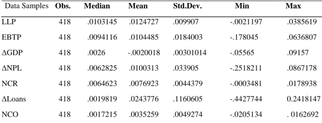
Table 2 below displays descriptive statistics of the variables after winsorizing outliers. The mean of loan loss provisions to outstanding loans is 1 percent, which is about the same as found in previous research (Anandarajan, Hasan, and McCarthy 2007). Neither of the remaining statistics deviate significant from findings in other the previous studies. Appendix 5 provides tables with the descriptive statistics of the data sample divided into pre-Basel 3 and post-Basel 3.
Table 2: Descriptive Statistics
Data Samples Obs. Median Mean Std.Dev. Min Max
LLP 418 .0103145 .0124727 .009907 -.0021197 .0385619 EBTP 418 .0094116 .0104485 .0184003 -.178045 .0636807 ΔGDP 418 .0026 -.0020018 .00301014 -.05565 .09157 ΔNPL 418 .0062825 .0100313 .033905 -.2518211 .0867178 NCR 418 .0064623 .0076923 .0044379 -.0003481 .0178938 ΔLoans 418 .0019819 .0243776 .1160605 -.4427744 0.2418147 NCO 418 .0017215 .0035259 .0049274 -.0205134 . 0162692
19 5.5 Regression Analysis
Estimation Methods
Panel data regression can be tested by three different types of models: Pooled ordinary least square (OLS), fixed effects (FE) and random effects (RE) model. To test which of the models that will give the most accurate results, I performed validity tests, using Breusch-Pagan Lagrange multiplier (LM) and Hausman (Torres-Reyna 2007).
Breusch-Pagan Lagrange multiplier (LM)
The LM is used for testing for random effects, and helps us to decide between using a random effects regression or a simple pooled OLS regression. The null hypothesis in the LM test is that the variance across entities is zero, hence no significant difference across units. Thus, if the LM test is significant, we will use the RE model instead of the OLS model (Torres-Reyna 2007). In this test, I found that the test was significant. Hence, RE model is better that OLS (Appendix. 1.1).
Hausman Test
When deciding between using the FE and RE model, I apply a Hausman test. Here the null hypothesis is that the preferred model is the RE, versus the alternative the FE. The Hausman test basically tests whether the unique errors terms are correlated with the regressors, and the null hypothesis is that they are not. Consequently, if the Hausman test is insignificant we will use the RE model, and if it is significant we will use the FE model (Torres-Reyna 2007). The results were significant, which implies that the FE model is better to run than the RE model (Appendix 1.2). As observed from the LM and Hausman tests, we can clearly see that the FE model is the most suitable estimation model for running the regression with my data sample.
20 5.6 Regression Diagnostics
Heteroscedasticity
In order to estimate reliable regression models, it is of crucial not to violate some fundamental assumptions regarding the residuals. One of them is the assumption of homoscedasticity, which means that the residual has equal disturbance variance 𝑞𝑞2 between units observed. According to the results presented in appendix 1.3, we can see that my result is in favor of rejection of the null hypothesis of homoscedasticity. This implies that there do exists a problem with heteroscedasticity.
Autocorrelation
When analyzing data over time, the problem with autocorrelation often occurs. If the error terms are correlated across time, the hypothesis testing is not reliable. Serial correlation causes the results to be less efficient, due to bias standard error. Thus, in order to have valid estimators I need to check for autocorrelation and eventually take necessary precautions (Gujarati 2011). The test and its results are presented in appendix 1.4, and show a presence of autocorrelation.
Multicollinearity
Multicollinearity among the explanatory variables can lead to large variances and covariances, which can widen the confidence intervals. As a result, statistical inference become harder to make since the impact of individual variables is hard to identify. When I tested my data, I found no discount in the result values. Hence, there is no proof for multicollinearity (Appendix. 1.5).
Checking Normality of Residuals
This procedure involves examining if the residuals are normally distributed in the models. Furthermore, I visually inspect the residual’s distribution by examining the plotted graph of the estimated residuals. The distribution showed in Appendix. 1.6, does not differ significantly from the normal distribution expectation. Moreover, I found that the residual is normally distributed.
21
6.0 Analysis and Result Discussion
From the conclusions of the tests and diagnostics conducted in the previous section, I find that the best suitable model to perform the regression in will be a fixed effects, cluster model (xtreg FE cluster). This controls for heteroscedasticity and autocorrelation, which both are present in the data. 6.1 EBTP-Model
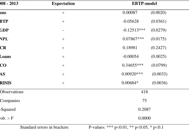
Table 3 below presents the results for the first regression model (EBTP-model) where I test for earnings management for the whole period (2008-2013) without including the interaction variable representing the implementation of the third Basel Accord (EBTP*BAS). The result says that the 𝑁𝑁2 = 23,79%. However, the results for EBTP, NCR and ΔLoans are statistically insignificant,
which means that also the explanation degree is not statistically correct.
Table 3: Results of FE Cluster regression of EBTP-Model of LLP
2008 - 2013 Expectation EBTP-model Cons + 0.00087 (0.0020) EBTP + -0.05628 (0.0361) ΔGDP - -0.12513*** (0.0279) ΔNPL + 0.07867*** (0.0175) NCR + 0.18981 (0.2427) ΔLoans + -0.00054 (0.0025) NCO + 0.34655*** (0.0799) BAS + 0.00920*** (0.0033) CRISIS + 0.00684* (0.0036) # Observations # Companies R-Squared Prob. > F 418 75 0.2087 0.0000 Standard errors in brackets P-values: *** p<0.01, ** p<0.05, * p<0.1
22 All though some of the result are not statistically significant, the results still indicates that these variables have an effect on LLP. We can see that the EBTP coefficient is -.05628. As stated earlier, I expected this to be positive, in which would represent a presence of earnings smoothing activity in the respective time-period. Nevertheless, this negative number implies that for every percent the EBTP increases, the respective year’s LLP will decrease by 5.628%. This tells us that the relationship between these two variables is opposite of what a EM-relationship implies. Thus, there is no proof of earnings smoothing during 2008-2013 in the European banks in the data sample that I have collected for this research. Previous research that is done within the same period, have found other evidence. Stoian and Norden (2013) found evidence for EM in the years 1999-2011, Gombola, Yueh-fang Ho, and Huang (2016) shows a presence of EM in banks during 1999-2013, Magnis and Iatridis (2017) finds evidence for a limited, but still present, EM activity after implementation of Basel II, Ozili (2017b) state that income smoothing is an incentive for EM in the post-crisis period, and (Garsva, Skuodas, and Rudzioniene 2012) finds evidence for it between 2005-2010. I have not yet found any research that find the same results as me in European banks during this period. One reason may be that none of these studies focus on the same year span as I have included. Another reason may explanatory factor may be the doubtfulness validity of the results due to the high p-value of this variable, making it statistically insignificant.
The control variables ΔGDP, ΔNPL, NCR and NCO are all giving expected results. ΔGDP has a coefficient of -.1251 which tells us that the LLP will decrease with an increase in the respective country’s GDP. This is a logical relationship, where banks will provision less if their country experience national economic growth. The result is proven to be statistically significant at a confidence level of 99%. Another significant result, is ΔNLP with a positive coefficient of 7,87% with a confidence level of 99%. As stated earlier, this also represent a logical relationship to LLP.
23 Non-performing loans gives an understanding of the risk of default of the bank’s outstanding loans, hence, its credit risk. The correlation is conveying that the bank’s provision is higher when there is an increase in the default risk, which is according to what one can expect from the behavior of provisioning activities. The results of both these variables are in line with the previously discussed pro-cyclicality behavior of banks (Skala 2015), where they tend to provision higher in tough economic times which implies a higher credit risk, and less when the economy is growing, as represented by an increase in the country’s GDP.
Both NCR and NCO have high effects on LLP. The result says that one percentage increase in NCR will increase the LLP with 18,98%. Though this is not significant, it still indicates that banks with high commission revenue, tends to set higher provisions. As mentioned before, Hasan and Hunter (1999) argue that this is done to signal that the bank is solid. The high positive correlation between NCO and LLP (35,65%) is significant at a 99% confidence level. It conveys that the LLP will increase with 35,65% for every percentage increase in NCO. This relationship is expected, as a higher provisioning will replace the “charge offs” that is written down in the loan loss reserves. ΔLoans does not have an expected effect on LLP. The coefficient is negative, which tells us that the provisions decrease as the bank lend out more money. However, the correlation is very weak, only -0.05% with a std. error of 0.2%. Taking into consideration the size of the coefficient, the std. error is significantly large. One can question if this small correlation can be defined as negative, or rather closer to zero. Moreover, the effect of changes in loans on LLP is relatively minimal. Both dummy-variables BAS and CRISIS, show a positive relationship to LLP. This proves that both during the financial crisis and post-Basel3, the LLP increased 0.68% and 0.92%, respectively. As explained earlier, these are natural provisioning behavior of the banks considering the changes in the financial markets and the capital regulations in which these dummy-variables represent.
24 6.2 Basel III-Model
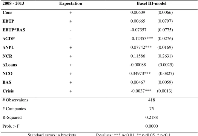
Table 4: Results of FE Cluster regression of Basel III-Model of LLP
2008 - 2013 Expectation Basel III-model
Cons + 0.00609 (0.0066) EBTP + 0.00665 (0.0797) EBTP*BAS - -0.07357 (0.0775) ΔGDP - -0.12353*** (0.0276) ΔNPL + 0.07742*** (0.0169) NCR + 0.11586 (0.2631) ΔLoans + -0.00088 (0.0025) NCO + 0.34973*** (0.0827) BAS + 0.00467 (0.0059) Crisis + -0.0037*** (0.0013) # Observaions # Companies R-Squared Prob. > F 418 75 0.2188 0.0000 Standard errors in brackets P-values: *** p<0.01, ** p<0.05, * p<0.1
In the second regression model (Basel III-model), I include the interaction variable EBTP*BAS, which provides an understanding of how the third Basel Accord impact the correlation between EBTP and LLP. In table 4 above we find the results of this regression. The 𝑁𝑁2 = 24,97%, which means that this model provides a little higher degree of explanation than the EBTP-model. As we see from the table, only three out of ten estimates are statistically significant. I can therefore not say that the model and the effects of all the included variables are true with a high level of confidence, but I still recognize that there exist indications for effects. I further conclude that in this specific data sample that I have collected, there is no statistical significant evidence that the implementation of the third Basel Accord influenced earnings smoothing using loan loss provisions. This advocate for keeping the H0, stating no effect on EM. However, the interaction
25 estimate does show an effect on EM activity using LLPs, even though it is not statistically significant. This indicates that the improvements in the third Basel Accord reduced the aggressiveness of earnings smoothing by 7,35% in the post-Basel3 years. When further examining the plot of the relation between EBTP*BAS and LLP (Appx. 2.2), the pattern is not clearly presented, but we can see that there is a slightly stronger pattern of a negative correlation, than a positive one. This is presented by a higher density of the sample in the lower right corner (high EBTP and lower LLP), than in the upper right (high EBTP and high LLP).
7.0 Conclusions, limitations and further research
In this master thesis, I have applied widely used explanatory variables from the research practice on earnings management using loan loss provisions in listed European banks. The purpose was to look at the effect of the regulatory improvements from the second Basel Accord to the third, in an attempt to contribute to a better understanding of the discretionary behavior of loan loss provisioning. In addition, to see if international regulation enhancements can have a positive effect on this behavior, as an aggressive EM may have negative consequences on regulations’ purpose. Most of the results I found was not statistically significant, but did, however, indicate that the independent variables had effects on LLP. The main findings include the EBTP-model showing indications of a negative correlation between EBTP and LLP. This implies that during 2008-2013, earnings and provisioning have an opposite relationship than what an earnings smoothing-relation would show. Most of the control variables showed expected results, except for ΔLoans which only had a minimal effect. The Basel III-model showed that the implementation of the enhancements in the Basel Accord reduced the EM activity by 7.35% in the three following years, even though this result was not statistically significant. In conclusion, I did not find a statistical significant evidence for rejecting the H0, but there are still indications stating that Basel III reduced the EM activity.
26 Because of the high p-values, one can question the validity of these results. I consequently think this effect should be tested for in a more comprehensive study, with an extended sample. One suggestion is to include a greater year span. The implication of this is that you then may have to include years before 2008, in which only the first Basel Accord was implemented. Thus, you will then look at the effect of the Basel III, against both Basel I and II. Another suggestion is to expand number of banks. This can be difficult as you need certain accounting information that is lacking among some of the banks. This may also mean you need to include unlisted or private banks in which are not obligated to report under IFRS. Further this can lead to a causality problem, because reporting standards can be an essential factor in provisioning behavior.
The results of my research may to some degree depend on the statistical estimation model. I used a fixed effect cluster model in which I found was the most suitable for this data sample, according to the tests discussed in section five. I am positive that a 100% explanatory model for LLP is much more complex than the one I have proposed, as the determinations of LLP estimates is based on assumptions, methodology and other unobservable managerial choices (Ozili 2017a). This is where the strength of the FE model comes in, as it eliminates omitted variable bias when unobservable variables are present. A significant limitation with this model, however, is that it cannot include the effect of variables with little variation within one bank over the year span (Blumenstock 2003). Further research should, as mentioned, include a more comprehensive data sample to see if the indicated effect of Basel III is significant. Other further research may include several incentives for provisioning such as capital management, signaling and capital risk. These have been widely researched previously, however very little, if not none, on the current Basel Accord. The interesting part of looking at LLP’s activity incentivized by credit risk, is to examine how pro-cyclical banks are, and the degree of fulfillment of capital regulation’s purpose.
27
8.0 References
Ahmed, Anwer S., Michael Neel, and Dechun Wang. 2013. “Does Mandatory Adoption of IFRS Improve Accounting Quality? Preliminary Evidence.” Contemporary Accounting Research 30 (4): 1344–72. doi:10.1111/j.1911-3846.2012.01193.x.
Ahmed, Anwer S., Carolyn Takeda, and Shawn Thomas. 1999. “Bank Loan Loss Provisions: A Reexamination of Capital Management, Earnings Management and Signaling Effects.”
Journal of Accounting and Economics 28 (1): 1–25. doi:10.1016/S0165-4101(99)00017-8.
Anandarajan, Asokan, Iftekhar Hasan, and Cornelia McCarthy. 2007. Use of Loan Loss Provisions
for Capital, Earnings Management and Signalling by Australian Banks. Accounting and Finance. Vol. 47. doi:10.1111/j.1467-629X.2007.00220.x.
Andrews, Charles, Francois Grunenwald, Fernando de la Mora, and Shyam Venkat. 2010. “The New Basel III Framework : Navigating Changes in Bank Capital Management.”
Basel Committee on Banking Supervision. 2013. “Complete Set of Agreed Changes to the Formulation of the Liquidity Coverage Ratio Published in December 2010.” Working Paper,
Bank for International Settlemens.
———. 2014. “Basel III: The Net Stable Funding Ratio.” Working Paper, Bank for International
Settlemens.
———. 2015. “The Interplay of Accounting and Regulation and Its Impact on Bank Behaviour: Literature Review.” Working Paper, Bank for International Settlemens. http://www.bis.org/bcbs/publ/wp28.pdf.
Basel Committee On Banking Supervision. 2011. “Basel III: A Global Regulatory Framework for More Resilient Banks and Banking Systems.” Working Paper, Bank for International
Settlemens. http://www.bis.org/publ/bcbs189.pdf.
Baum, Christopher F. 2001. "Residual diagnostics for cross-section time series regression models."
The Stata Journal: 101-104.
Blumenstock, Joshua. 2003. “Fixed Effects Models.”
Bushman, Robert M., and Christopher D. Williams. 2012. “Accounting Discretion, Loan Loss Provisioning, and Discipline of Banks’ Risk-Taking.” Journal of Accounting and Economics 54 (1). Elsevier: 1–18. doi:10.1016/j.jacceco.2012.04.002.
Cavallo, Michele, and Giovanni Majnoni. 2001. “Do Banks Provision for Bad Loans in Good Times?”
Collins, Julie H, Douglas A Shackelford, and James M Wahlen. 1995. “Bank Differences in the Coordination of Regulatory Capital, Earnings, and Taxes.” Journal of Accounting Research 33 (2): 263–91. doi:10.2307/2491488.
Curcio, Domenico, and Iftekhar Hasan. 2015. Earnings and Capital Management and Signaling:
The Use of Loan-Loss Provisions by European Banks. The European Journal of Finance. Vol.
28 Daske, Holger, Luzi Hail, Christian Leuz, and Rodrigo Verdi. 2008. “Mandatory IFRS Reporting around the World: Early Evidence on the Economic Consequences.” Journal of Accounting
Research 46 (5): 1085–1142. doi:10.1111/j.1475-679X.2008.00306.x.
Dechow, Patricia M., Richard G. Sloan, and Amy P. Sweeney. 1995. “Detecting Earnings Management.” The Accounting Review 70 (2): 193–225. doi:10.2307/248303.
Defond, Mark L, and Chul W Park. 1997. “Smoothing Income in Anticipation of Future Earnings.”
Journal of Accounting and Economics 23 (2): 115–39. doi:10.1016/S0165-4101(97)00004-9.
Duru, Keneth, and Alexandros Tsitinidis. 2013. “Managerial Incentives and Earnings Management: An Empirical Examination of the Income Smoothing in the Nordic Banking Industry.” Uppsala University.
Finch, Niegel. 2009. “IAS 39 and the Practice of Loan Loss Provisioning Thoughout Australasia.”
Journal of Law and Financial Managment 8 (2): 13–19.
Fonseca, Ana Rosa, and Francisco González. 2008. “Cross-Country Determinants of Bank Income Smoothing by Managing Loan-Loss Provisions.” Journal of Banking and Finance 32 (2): 217–28. doi:10.1016/j.jbankfin.2007.02.012.
Fudenberg, Drew, and Jean Tirole. 1995. “A Theory of Income and Dividend Smoothing Based on Incumbency Rents.” Journal of Political Economy 103 (1): 75–93. doi:10.1086/261976. Frees, Edward W. 2004. Longitudinal and panel data: analysis and applications in the social
sciences: Cambridge University Press.
Garsva, Gintautas, Sigitas Skuodas, and Kristina Rudzioniene. 2012. “Earnings Management in European Banks : The Financial Crisis and Inceased Incentives for Manipulation through LLPs.” Transformations in Busiiness and Economics 11: 42–59.
Ghosh, Dhiren, and Andrew Vogt. 2012. “Outliers: An Evaluation of Methodologies.” Joint
Statistical Metings, 3455–60.
Gombola, Michael J, Amy Yueh-fang Ho, and Chin-chuan Huang. 2016. “The Effect of Leverage and Liquidity on Earnings and Capital Management : Evidence from U . S . Commercial Banks.” International Review of Economics and Finance 43 (200): 35–58. doi:10.1016/j.iref.2015.10.030.
Greenawalt, Mary Brady, and Joseph F. Sinkey. 1988. “Bank Loan-Loss Provisions and the Income-Smoothing Hypothesis: An Empirical Analysis, 1976-1984.” Journal of Financial
Services Research 1 (4): 301–18. doi:10.1007/BF00235201.
Gujarati, Damodar. 2014. Econometrics by example. Palgrave Macmillan
Hasan, I., and W. C. Hunter. 1999. "Income-smoothing in the depository institutions: An empirical investigation." Advances in Quantitative Analysis of Finance and Accounting 1-16.
Healy, P M, and J M Wahlen. 1999. “A Review of the Earnings Management Literature and Its Implications for Standard Setting.” Accounting Horizons 13 (4): 365–83. doi:10.2308/acch.1999.13.4.365.
29 Jones, Jennifer J. 1991. “Earnings Management During Import Relief Investigations.” Journal of
Accounting Research 29 (2): 193–228. doi:10.2307/2491047.
Kanagaretnam, Kiridaran, Gerald J. Lobo, and Robert Mathieu. 2004. “Earnings Management to Reduce Earnings Variability: Evidence from Bank Loan Loss Provisions.” Review of
Accounting and Finance 3 (1): 128–48. doi:10.1108/eb043399.
Laeven, Luc, and Giovanni Majnoni. 2003. “Loan Loss Provisioning and Economic Slowdowns: Too Much, Too Late?” Journal of Financial Intermediation 12 (2): 178–97. doi:10.1016/S1042-9573(03)00016-0.
Leventis, Stergios, Panagiotis E. Dimitropoulos, and Asokan Anandarajan. 2011. “Loan Loss Provisions, Earnings Management and Capital Management under IFRS: The Case of EU Commercial Banks.” Journal of Financial Services Research 40 (1–2): 103–22. doi:10.1007/s10693-010-0096-1.
Lobo, Gerald J. 2016. “Accounting Research in Banking – A Review.” China Journal of
Accounting Research 10: 1–7. doi:10.1016/j.cjar.2016.09.003.
Magnis, Chris, and George Emmanuel Iatridis. 2017. “The Relation between Auditor Reputation, Earnings and Capital Management in the Banking Sector: An International Investigation.”
Research in International Business and Finance 39: 338–57. doi:10.1016/j.ribaf.2016.09.006.
Oosterbosch, Renick Van. 2010. “Earnings Management in the Banking Industry.” Erasmus MC:
University Medical Center Rotterdam.
Ozili, Peterson K. 2017a. “Bank Loan Loss Provisions Research: A Review.” https://ssrn.com/abstract=2905874.
Ozili, Peterson K. 2017b. “Discretionary Provisioning Practices among Western European Banks.”
Journal of Financial Economic Policy 9 (1): 109–18. doi:10.1108/JFEP-07-2016-0049.
Perry, Brian. “Understanding the Basel 3 International Regulations”. Investopedia. 2013.
Skala, Dorota. 2015. “Saving on a Rainy Day? Income Smoothing and Procyclicality of Loan-Loss Provisions in Central European Banks.” International Finance 18 (1): 25–46. doi:10.1111/1468-2362.12058.
Spitteler, Evelien. 2011. “Loan Loss Provisions , Capital Management and Earnings Management under Basel II : Evidence from European Commercial Banks.” Amsterdam Business School. Stoian, Anamaria, and Lars Norden. 2013. “Bank Earnings Management through Loan Loss
Provisions: A Double-Edged Sword?” http://www.dnb.nl/en/binaries/Working Paper No 8-2004_tcm47-146665.pdf.
Torres-Reyna, Oscar. "Panel data analysis." Fixed & Random Effects. 2007.
Tucker, Jennifer, and Paul Zarowin. 2006. “Does Income Smoothing Improve Earnings Informativeness?” The Accounting Review 81 (1): 251–70.
Wall, L. D. and Koch, T. W. 2000. “Bank Loan-Loss Accounting: A Review of Theoretical and Empirical.” Federal Reserve Bank of Atlanta Economic Review Second Qua: 1–19.
30 Williams, Richard. 2015. "Multicollinearity." Multicollinearity.
Wooldridge, Jeffrey M. 2002. “Econometric Analysis of Cross Section and Panel Data” MIT Press Zaher, Fadi. "How Basel 1 Affected Banks". Investopedia. 2007.