Universidade de Lisboa
Faculdade de Ciências
Departamento de Biologia Animal
Thermal Tolerance and Sensitivity of
Amphibian Larvae from Paleartic and
Neotropical Communities
Marco Jacinto Katzenberger Baptista Novo
Mestrado em Biologia da Conservação
2009
i
Universidade de Lisboa
Faculdade de Ciências
Departamento de Biologia Animal
Thermal Tolerance and Sensitivity of
Amphibian Larvae from Paleartic and
Neotropical communities
Marco Jacinto Katzenberger Baptista Novo
Mestrado em Biologia da Conservação
2009
Dissertação orientada por
Dr. Miguel Tejedo
Department of Evolutionary Ecology, Doñana Biological Station, CSIC
e
Prof. Rui Rebelo
Departamento de Biologia Animal, Faculdade de Ciências, Universidade de
Lisboa
ii
To Maria, Jacinto and Manuela
Thank you for making my life such a wonderful and exciting ride!
Rhinella schneideri, (Werner, 1894)
On the cover – Rhinella granulosa, (Spix, 1824)
iii
“All over the world the wildlife that I write about is in grave danger. It is
being exterminated by what we call the progress of civilization. (…) Does a
creature have to be of direct material use to mankind in order to exist? By
and large, by asking the question "what use is it?" you are asking the
animal to justify its existence without having justified your own.”
Gerald Durrell
“We can't leave people in abject poverty, so we need to raise the standard
of living for 80% of the world's people, while bringing it down considerably
for the 20% who are destroying our natural resources.”
Jane Goodall
iv
ABSTRACT
Amphibians across the world are threatened by climate change. This work deals with the analysis of thermal tolerance and sensitivity and their latitudinal variation at the community level, with the intent of examining the prediction that tropical amphibians are at higher risk of extinction due to global warming than temperate species since their environmental temperatures are closer to their upper thermal limits.
To test this prediction, two larval amphibian communities were selected from contrasting latitudes: subtropical (Argentina) and temperate Mediterranean (Iberian Peninsula) climates. In both locations, the following key parameters were obtained: 1) environmental pond temperatures (Thab), by monitoring ponds at different locations using water dataloggers; 2) critical thermal maximum, using a dynamic method called CTmax or knockdown temperature, to assess how close environmental temperatures are from their upper thermal limit; and 3) optimum temperature (Topt), by analysing tadpole’s maximum swimming speed at different temperatures and building thermal performance curves (TPCs), to determine how changes in environmental temperatures will affect the ability to perform ecologically relevant functions and therefore their general fitness.
Warming Tolerance (WT) (WT=CTmax-Thab) and Thermal Safety Margins (TSM) (TSM=Topt-Thab) were also calculated for all species.
Analyses of CTmax and optimal performance temperature indicate that species have adapted their critical and optimal temperatures to cope with environmental conditions. Species exposed to higher maximum or average temperatures usually have higher CTmax or optimum temperatures, respectively. In addition, there is a significant positive correlation between these traits.
Results also show that Argentinean subtropical species, although having higher CTmax and optimum temperature values, have lower WT and narrower TSM. Therefore, these species generally appear to be in greater extinction risk than temperate species from the Iberian Peninsula, under predicted scenarios of rising temperatures and climate change.
Keywords: thermal tolerance, thermal sensitivity, performance, global warming,
v
RESUMO
Este trabalho aborda a questão de como os organismos irão lidar com a ameaça do aquecimento global. Seleccionaram-se os anfíbios como objecto de estudo por estes serem o grupo de vertebrados terrestres mais ameaçado e por potencialmente serem altamente sensíveis aos efeitos da subida da temperatura. A sua ectotermia, fase larvar aquática e mobilidade limitada poderão aumentar o impacto que o aquecimento global terá nos anfíbios e nas suas populações. Pretendeu-se abordar esta complexa questão através de uma análise de duas comunidades, procurando desvendar se espécies de anfíbios sujeitas a regimes térmicos distintos, por exemplo comunidades de anfíbios tropicais “versus” temperadas, diferem no risco de extinção face aos desafios impostos pelos cenários previstos de mudança climática.
Analisaram-se a tolerância e a sensibilidade térmicas, ao nível específico e de toda a comunidade, e a sua variação latitudinal. Examinou-se a previsão de que os anfíbios tropicais se encontram sujeitos a um risco de extinção mais elevado devido ao aquecimento global do que as espécies temperadas, uma vez que as temperaturas ambientais a que estão sujeitos estão mais perto dos seus limites térmicos superiores.
De modo a testar esta previsão, seleccionaram-se duas comunidades de larvas de anfíbios, abrangendo os climas subtropical (Argentina) e temperado mediterrânico (Península Ibérica). Para cada comunidade, foram obtidos os seguintes parâmetros-chave: temperaturas ambientais das charcas; temperatura crítica máxima (CTmax) de uma selecção de espécies, para determinar a proximidade do seu limite térmico máximo às temperaturas ambientais; e curvas de “performance” térmica (TPCs) durante a fase larvar, de modo a perceber como as temperaturas ambientais afectam a sua capacidade de realizar funções ecologicamente relevantes e, portanto, a sua “fitness” geral.
Para a comunidade subtropical, seleccionaram-se áreas de estudo no norte da Argentina. Foram incluídas charcas da região do “El Gran Chaco”, províncias de Formosa e Chaco, e também da parte norte da província de Corrientes, abragendo uma área geográfica entre 24-27ºS e 58-61ºW. Estas regiões caracterizam-se por um regime sazonal de precipitação, concentrada durante o verão austral, o que condiciona os anfíbios a reproduzirem-se num período especialmente quente e húmido. O “El Gran Chaco” é , inclusive, uma das regiões mais quentes da América do Sul.
As áreas de estudo para a comunidade temperada de anfíbios situaram-se na Península Ibérica, onde os girinos foram recolhidos em Portugal e Espanha, cobrindo uma distribuição norte-sul desde Oviedo, Astúrias (43ºN), até Doñana, Andaluzia (37ºN), e uma distribuição este-oeste desde Granada, Andaluzia (3ºW), até Verdizela, na costa portuguesa (9ºW). A maioria dos anfíbios da Península Ibérica reproduz-se com temperaturas mais frias, durante o Outono, Inverno e/ou Primavera; apenas as espécies que vivem a altitudes mais elevadas se reproduzem no início do Verão.
De modo a estimar a tolerância ao aquecimento e as margens de segurança térmicas, são necessários dados ambientais sobre a temperatura da água das charcas.
vi
Para a monitorização dos perfis térmicos dos habitats de reprodução, colocaram-se “dataloggers” para água no fundo das charcas (zona fria) e na margem (zona quente), de modo a obter todo o gradiente térmico existente. No total, foram monitorizadas 20 charcas.
No total, estudaram-se 19 espécies quanto à sua tolerância e sensibilidade térmicas: 9 da comunidade subtropical na Argentina (Pseudis limellum, Pseudis
paradoxa, Scinax acuminatus, Scinax nasicus, Elachistocleis bicolor, Trachycephalus venulosus, Hypsiboas raniceps, Leptodactylus latinasus, Leptodactylus bufonius e Physalaemus albonotatus) e 9 da comunidade temperada da Península Ibérica
(Pelobates cultripes, Pelodytes ibericus, Alytes cisternasii, Alytes dickhilleni, Rana
temporaria, Rana iberica, Hyla meridionalis, Hyla arborea and Epidalea calamita).
Os limites máximos de tolerância térmica foram determinados usando um método dinâmico designado por CTmax ou temperatura de “knockdown”. Foram testados 15-20 girinos por espécie, em laboratório. Os animais estiveram no mínimo 4 dias à temperatura de aclimatização de 20°C e foram mantidos em recipientes de plástico, a uma densidade larvar semelhante, com um fotoperíodo de 12D:12L e alimentadas “ad libitum”. Determinou-se o CTmax aquecendo os girinos a uma taxa de 1 ºC/min. Colocou-se cada larva em 400 ml de água sem cloro numa taça de vidro de 700 ml parcialmente submergida dentro de um recipiente de 2000 ml. A água no recipiente maior foi aquecida uniformemente por um agitador magnético Agimatic‐N (P‐Selecta). Cada teste começou à temperatura de aclimatização. Monitorizou-se a temperatura da água com um termómetro digital (digi‐thermo) (± 0,1°C). Registou-se a perda de “righting response” (LRR) e o início dos espasmos (OS). Uma vez atingido o OS, o girino foi colocado em água fria para permitir a sua recuperação.
Para estimar a sensibilidade térmica foram construídas curvas de “performance” térmica para cada espécie (TPCs). Estas TPCs foram baseadas na capacidade locomotora medida como “burst swimming” nos girinos. Utilizou-se um canal de metacrilato, no qual as larvas nadaram a temperatura controlada. Cada girino foi colocado no canal e estimulado com uma vareta fina até que produzisse um “burst swim”. Os testes foram gravados com uma câmara de video digital, colocada 2 m acima do canal. Foram testadas 15-20 larvas por espécie, com aclimatização igual à do CTmax, às temperaturas de 20°, 24°, 28°, 32°, 35° e 38°C para as espécies argentinas e de 10°, 15°, 20°, 24°, 28°, 32° e 35°C para as espécies ibéricas. Algumas espécies argentinas não toleram aclimatização a 20°C (por exemplo, alguns Leptodactilídeos) pelo que se considerou que as temperaturas inferiores a 20°C pudessem estar fora do intervalo de “performance” locomotora natural para esta comunidade. O mesmo argumento justifica a temperatura máxima testada nas comunidades paleárticas.
A relação entre tolerância térmica, sensibilidade e temperatura de habitat foi examinada num contexto filogenético, de modo a determinar até que ponto os padrões observados poderão derivar estritamente de um fundo genético comum entre espécies próximas. Como tal, foi usado o teste TFSI (“test for serial independence”)
vii
para caracteres contínuos e o método de PIC (“phylogenetically independent contrasts”) para determinar se cada caracter estava significativamente associado à sua história filogenética e para corrigir as correlações encontradas tendo em conta a sua filogenia.
As espécies de anfíbios da Argentina apresentaram, em geral, um valor de CTmax mais elevado que as espécies da Pensínsula Ibérica. À escala global, para as 19 espécies estudadas, os limites térmicos máximos de tolerância reflectiram as condições ambientais. Tanto antes como depois de corrigir pela filogenia, obteve-se uma correlação significativa entre as temperaturas ambientais e os limites térmicos máximos de tolerância.
Quanto à temperatura óptima de “performance”, os resultados foram semelhantes aos das análises dos limites térmicos máximos. Em geral, as espécies argentinas possuem um valor óptimo de temperatura mais elevado que as espécies ibéricas. Porém, existe muita variabilidade para este caracter nas espécies da Península Ibérica. Com base nessa variabilidade, foi possível discriminar dois grupos: espécies que se reproduzem na Primavera e princípios de Verão, com valores de óptimo bastante semelhantes aos das espécies argentinas; e espécies que se reproduzem no Outono/Inverno e/ou em habitats frios (ribeiras ou montanha), com valores de óptimo claramente inferiores aos das espécies subtropicais.
Os resultados indicaram também que as espécies adaptaram a sua temperatura óptima de modo a lidar com as condições ambientais locais, pelo que existe uma correlação significativa entre temperatura óptima e temperatura média ambiental.
Tanto para o Ctmax como para a temperatura óptima de “performance”, espécies expostas a temperaturas ambientais mais elevadas possuem valores também mais elevados para estes dois caracteres.
As espécies de anfíbios da Argentina, apesar de possuírem valores de CTmax e de temperatura óptima mais elevados, têm menor tolerância ao aquecimento e margens de segurança térmica mais estreitas que as espécies da Península Ibérica. Portanto, num cenário de mudança climática, em que se prevê um aquecimento global, as espécies de anfíbios subtropicais estarão em maior risco de extinção que os anfíbios de regiões temperadas.
Palavras-chave: tolerância térmica, sensibilidade térmica, aquecimento global,
viii
INDEX
1. Introduction 1
1.1. State of the art 1
1.2. Objectives and study organisms 4
1.3. Thermal tolerance studies 7
1.4. Thermal sensitivity studies 8
2. Methodology 10
2.1. Field work 10
2.1.1. Study areas 10
2.1.2. Monitoring environmental temperatures 11
2.2. Comparative evaluation of the upper thermal maxima and
Warming Tolerance 12
2.3. Evaluation of thermal sensitivity of locomotor performance and
Thermal Safety Margins 14
2.4. Phylogenetic analyses 15
3. Results 17
3.1. Monitoring environmental temperatures 17
3.2. Upper thermal maxima and Warming Tolerance 20
3.3. Thermal sensitivity and Thermal Safety Margins 24
3.4. CTmax vs Optimum Temperature and Warming Tolerance vs
Thermal Safety Margins 30
4. Discussion 33
4.1. Thermal tolerance 33
4.2. Thermal sensitivity 34
4.3. Evaluating vulnerability to warming temperatures 35
5. Acknowledgments 38
6. References 40
7. Annexes 47
Annexe I. Monitored ponds 47
Annexe II. Phylogenetic trees 48
Annexe III. CTmax 50
- 1 -
1. INTRODUCTION 1.1. State of the art
Temperature affects virtually all physiological processes. It determines both rates of chemical reactions (Hochochka and Somero, 2002) and many ecological interactions (Dunson and Travis, 1991). Therefore, it is expected that environmental temperature changes associated with global warming will have broad ecological consequences for species and communities (Southward et al., 1995; Pearson and Dawson, 2003; Case et al., 2005). Recent reports, using meta‐analyses, have presented comprehensive synthesis of the impact of climate change on a range of species (Parmesan and Yohe, 2003; Root et al., 2003). However, extensive debate still exists on whether the observed biological changes can be conclusively linked to an anthropogenic effect on climate or contrarily it may be better attributed simply to sampling bias (Jensen, 2003).
To assess how climate change will really impact organims, deep knowledge is required on three main key issues: a) the current conditions and future climatic scenarios; b) how close organisms are to their thermal tolerance in nature; and c) to know the degree to which organisms are able to adjust or acclimatize their thermal sensitivity (Stillman, 2003; Gilman et al., 2006). One can expect that organisms with the greatest risk of extinction from rapid climatic change are those with a low tolerance to warming, limited acclimation ability and reduced dispersal, incapacitating them to avoid/adjust to new challenging conditions.
Ectotherms comprise most of the terrestrial biodiversity and are expected to be especially vulnerable to global warming since their basic physiological functions, development and behaviour are strongly affected by temperature. In these organisms, most physiological processes proceed rapidly over a range of body temperatures defining a thermal performance curve or TPC (Huey and Stevenson, 1979). This thermal sensitivity curve rises gradually from a minimum critical temperature (CTmin), to an optimum temperature (Topt), and then falls rapidly to a critical thermal maximum (CTmax). Critical thermal limits define the thermal tolerance range of an organism. Temperatures either below or above the range of tolerance result in impaired physiological function (Hillman et al., 2009).
Impacts of global warming on biodiversity are often assumed to be geographically dependent, being predicted to be smaller in the tropics relatively to those in temperate regions (Root et al., 2003; Parmesan, 2007) because the projected rate of climate warming in the tropics is lower than the one expected for higher latitudes (IPCC, 2007a). However, this prediction based on absolute temperature change may be misleading due to several factors associated with behaviour, physiology and ecology of organisms.
First, there are wide indications that thermal tolerance in different groups of ectotherms is related to the magnitude of temperature variation they normally experience (Janzen, 1969; Addo‐Bediako et al., 2000; Ghalambor et al., 2006), thereby
- 2 -
increasing with latitude. Most evidences suggest that temperate zone species should have relatively broad thermal tolerances (e.g. the difference between critical thermal minimum [CTmin] and maximum [CTmax]) than tropical ones, primarily because they are much more cold tolerant. Some available compilations of body temperatures are consistent with the prediction that their variability is reduced in the tropics and increases with latitude, for example in salamanders (Feder and Lynch, 1982), lizards (van Berkum, 1988) and crabs (Stillman and Somero, 2000).
Fig.1- Survival in a warmer climate. Data from diverse terrestrial ectotherms suggest that tropical species living in stable aseasonal climates, such as the Amazonian lizard Enyalioides palpebralis (top inset), have narrower thermal tolerances than do higher-latitude species such as the temperate lizard
Nucras tessellate (bottom inset), and also live in climates that are closer to their physiological optima.
The former may thus be highly vulnerable even to modest climate warming (in Tewksbury et al., 2008; Copyright © 2008 by the American Association for the Advancement of Science, Science).
Second, the impacts of environmental warming should be more negative on thermally specialized animals (Ghalambor et al., 2006) and/or on those that have a lower acclimation capacity (Stillman, 2003). From previous works, tropical ectotherms appear to be thermal specialists with lower acclimation capacity than higher‐latitude species (van Berkum, 1988; Addo‐Bediako et al., 2000; Hoffmann et al., 2003; Ghalambor et al., 2006; Gilman et al., 2006; Calosi et al., 2008; Deutsch et al., 2008).
- 3 -
Third, tropical ectotherms which are exposed to higher temperatures throughout the year might be expected to express higher heat tolerance. However, it seems that critical thermal maximum of terrestrial ectotherms does not vary much across latitude (Addo‐Bediako et al., 2000; Ghalambor et al., 2006; Deutsch et al., 2008; Tewksbury et al., 2008). Since many tropical ectotherms live in environments where body temperatures are close or even above optimal temperatures for performance (Deutsch et al., 2008), any small increment in temperature may have catastrophic consequences. These evidences suggest these species, constituting the richest faunistic biodiversity of the world, would be at a greater risk of extinction due to global warming comparing to species from higher latitudes. Nevertheless, a realistic evaluation of a higher geographic impact on the tropical ectotherms, due to predicted increase in temperatures, is lacking. This will need to combine both accurate knowledge of specific tolerance of organisms and the environmental temperature they are exposed to.
A vast majority of the research on thermal adaptation and thermal tolerance has been conducted on a few well‐studied model‐organisms, such as Drosophila sp., undergoing experimental stress under laboratory conditions (Hoffmann and Parsons, 1997; Hoffmann et al., 2003). In spite of this being a fundamental first step, the interest in producing information on focal threatened taxa, and specially those distributed across sensible habitats (e.g., amphibians in tropical and mountain areas), is rising as conservation actions will demand a higher level of knowledge of the physiological ecology and genetics of species in these particular systems.
Recently, Deutsch et al. (2008) provided a first quantitative assessment of this prediction, employing a physiological framework which integrated fitness curves, reflecting thermal tolerance of terrestrial insects from around the world, with projected geographic distribution of climate change, for the next century. To assess latitudinal variations in global warming impact on ectotherms, assuming that their basic physiological functions, such as locomotion, growth, development and reproduction, are heavily dependent on environmental temperature, two operative metrics were defined:
1. Warming tolerance (WT=CTmax–Thab), as the difference between the organism’s critical thermal maximum and the current temperature of its environment. This metric is related to the average warming that an ectotherm can tolerate before environmental temperatures reach its upper tolerance limit. The prediction is that tropical species would have lower WT than temperate or high‐latitude species.
2. Thermal safety margin (TSM=Topt–Thab), as the difference between the organism’s thermal optimum (Topt) and its current environmental temperature (Thab). The prediction was that tropical species would have a narrower TSM because they live at environmental temperatures closer to their physiological optimum. Therefore, any small increase in temperature could trigger a decrease in their performance. On the other hand, species from temperate or high‐latitude are exposed to cooler
- 4 -
temperatures than their optimal and, therefore, global warming may even increase their fitness and population growth rates.
Fig.2- Predicted impact of warming on the thermal performance of ectotherms in 2100. (A) Impact versus latitude for insects using thermal performance curves fit to intrinsic population growth rates measured for each species (black circles) and for a global model (red line) in which performance curves at each location are interpolated from empirical linear relationships between seasonality and both warming tolerance and thermal safety margin. (B and C) Results from the simplified conceptual model are shown globally for insects (B) for which performance data are most complete, and versus latitude for three additional taxa of terrestrial ectotherms: frogs and toads, lizards, and turtles (C), for which only warming tolerance was available (in Deutsch et al., 2008, fig. 3,© 2008 by The National Academy of Sciences of the USA).
Their results (figure 2) show that tropical insects and ectothermic vertebrates (reptiles and amphibians), despite being subjected to a lower increase in air temperatures, will suffer a large decrease in their fitness since they are currently living very close to their optimal temperature. Regarding species from higher latitudes, currently living in cooler temperatures, a changing climate may even benefit them.
However, this approach is opened to several criticisms. The major shortcomings of this approach are: first, habitat and body temperatures were estimated using only air temperature measurements of their habitats and thus disregarding the potential of thermoregulation of most ectotherms; and second, their estimates of CTmax were pooled from literature sources that did not control by acclimation and other factors that may induce bias on CTmax estimates (see Methodology 2.2.).
1.2. Objectives and study organisms
The main objective of this thesis is to assess whether tropical amphibians species (living normally under higher environmental temperatures) are at higher risk of extinction than temperate species (living normally under colder environmental temperatures) when facing global warming, since they are expected to exhibit both
- 5 -
lower warming tolerance (WT=CTmax–Thab) and narrower thermal safety margins (TSM=Topt–Thab).
Amphibians are considered the most endangered group of vertebrates since near one third of all extant species are threatened with extinction (Stuart et al., 2004). They have a number of physiological, ecological and life‐history characteristics that make them highly susceptible to environmental change such as ectothermy, permeable skin and complex life‐cycles (with metamorphosis), the last one presumed to be an adaptation to the sequential occupation of temporary wetlands and terrestrial environments (Wells, 2007). All of these traits also determine an important dependence on environmental factors and, in addition, can explain the geographic pattern of amphibian species richness. The tropics hold much higher species richness, containing more than 85 % of the current amphibian species (Duellmann, 1999; Wells, 2007; Stuart et al., 2008). Particularly, the Neotropical realm of Central and South America alone concentrates the highest diversity of amphibians on earth with 2916 recognized species, 49 % of world total (IUCN, 2006; Stuart et al., 2008).
Fig.3- Global diversity of amphibian species (in Global Amphibian Assessment, IUCN, 2006). Many of the reported cases of amphibian declines and extirpation of local populations have been caused by the pathogenic fungus Batrachochytrium
dendrobatidis (Stuart et al., 2004; Lips et al., 2006; Wake and Vredenburg, 2008), or
similar emergent diseases. Although it is unclear the extent to which global warming could have triggered devastating chytridiomicosis outbreaks (Rohr et al.,2008), there is mounting evidence that epidemic diseases may be driven by changes in the thermal environment (Pounds et al., 2006; Raffel et al., 2006; Bosch et al., 2007; Ruthig, 2008). So far, there has been no report on amphibian population decimation directly attributable to warming. Nevertheless, there is an obvious risk that the direct effects
- 6 -
of increasing temperatures and other manifestations of climate change can cause a second wave of extinctions in the mid/long‐term.
Fig. 4- Global distribution of threatened amphibians (in Global Amphibian Assessment, IUCN, 2006). See Global Amphibian Assessment for detailed maps of critical areas.
This work will look at the larval stage of amphibians. For several reasons, tadpoles can be considered a model organism for studying thermal tolerances in ectotherms, in general, and in amphibians, in particular:
1) The tadpole phase is a growth and developmental period and all analyzed traits are independent of reproductive condition;
2) Tadpoles are aquatic and their body temperatures are the same as the temperature of surrounding environment (Spotila et al., 1992);
3) Tadpoles living in water can not suffer the correlated dehydration response of terrestrial stages, when heating. However, they can suffer other stressors associated with increased temperature such as a decrease in water dissolved oxygen and subsequently in their aerobic performance (see Pörtner and Knust, 2007) or an increase in osmotic stress (Gómez‐Mestre and Tejedo, 2003, 2004) that may interact with thermal tolerances (Re et al. 2006);
4) Although tadpoles are capable of behaviourally regulating their body temperatures through selection amongst a range of available temperatures (Noland and Ultsch, 1981; Wollmuth et al., 1987; Hutchison and Dupré, 1992), their physical environments eventually limit the extent of their thermoregulation (Huey, 1974; Wu and Kam, 2005). This is particularly dramatic for tadpoles occupying temporary ponds because these are typically shallow and with small water volume and can suffer intense heating, especially those receiving direct sunlight, with important daily thermal gradients and without thermal stratification.
- 7 -
Fig.5- Tadpole of Pseudis paradoxa, (Linnaeus, 1758). Foto by Ricardo Reques.
In ponds located in tropical environments with a wet summer breeding season, tadpoles may be exposed to temperatures over 40°C. During heating waves, tadpoles may not be able to escape from dangerous temperatures before ponds dry completely, even though they are capable of behavioural thermoregulation (Wells, 2007), unless they can reach metamorphosis and jump to land. Here, a wider range of microhabitats can be found and possibly they will be able to select a more thermally favourable microclimate (Navas et al, 2007). The expected increase in global mean temperature, together with more frequent extreme hot events, such as heat waves, will accentuate this condition (IPCC, 2007b). On the other hand, global warming is predicted to shorten pond hydroperiods in many areas such as Central America and Australia due to parallel shortage in rainfalls (IPCC, 2007b) which may potentially increase local extinction of amphibian populations.
Most of the literature concerning temperature effects and responses has focused groups of ectothermic vertebrates other than amphibians (fish and reptiles). However, thermal physiology research in amphibians, in spite of seminal contributions in the 50s ‐ 70s (Brattstrom, 1959, 1962 and 1968; Lillywhite, 1970; Hutchison, 1961; Heatwole et al., 1965; Mahoney and Hutchison, 1969), has been intensively developed specially in later decades (see reviews in Rome et al., 1992; Hutchison and Dupré, 1992; Ultsch et al., 1999; Wells, 2007; Navas et al., 2008; Hillman et al., 2009).
1.3. Thermal tolerance studies
The analysis of thermal tolerances in amphibians was initially developed by Brattstrom (1968) in anurans, and Hutchison (1961), in salamanders. Interestingly, Brattstrom’s study included comparative data of CTmax for 53 species of frogs from a latitudinal and altitudinal gradient in North and Central America. He found that CTmax varied both at the species and population levels.
For most anuran larvae, CTmax was determined to fall between 38°C and 42°C (Ultsch et al., 1999). The differences in CTmax among populations may be a response
- 8 -
to interdemic thermal habitat through local genetic adaptation in thermal tolerance. A number of studies have demonstrated within species variation in heat tolerance (e.g., Hutchison, 1961; Brattstrom, 1968 and 1970; Delson and Whitford, 1973; Miller and Packard, 1977; Hoppe, 1978; Hertz et al., 1979; Garland and Adolph, 1991; Meffe et al., 1995; Schwarzkopf, 1998; Gvoždík and Castilla, 2001; Winne and Keck, 2005; Huang and Tu, 2008). However, few studies have performed common garden experiments designed to distinguish between genetic and acclimation induced differences in physiology (Garland and Adolph, 1991). In amphibians some evidences have been reported that CTmax may adaptively differ between populations (Skelly and Freidenburg, 2000; Chen et al., 2001; Wu and Kam 2005; C. Navas, unpublished data).
Other factors should be taken into account. Ontogeny may affect CTmax, which drops 3°C‐4°C when larvae are close to metamorphic climax (Floyd, 1983), requiring deeper analysis of maximum heating during this risk‐sensitive phase. Acclimation to higher temperatures may affect the estimate of CTmax, increasing its value up to 4°C (Brattstrom, 1968; Navas et al., 2008). It is recognized that CTmax exhibits a phylogenetic signal and differences between amphibian lineages can be found both in adult stages (Navas et al., 2008), and tadpoles, (H. Duarte and J.P. do Amaral, unpublished data).
Finally, some controversy exists whether CTmax is dependent on latitude. Analysis on insects revealed no geographical trend (Addo‐Bediako et al., 2000). In amphibians, the analysis of Brattstrom (1968) data set is inconclusive: Snyder and Weathers (1975) found a significant decline in CTmax with increasing latitude (r=0,70; p<0,05) whereas the re‐analysis of Ghalambor et al. (2006) showed that the trend was not significant (p >0,70).
Since estimates of CTmax are susceptible to error due to several factors, including variations in end‐points (Lutterschmidt and Hutchison, 1997), acclimation temperature (Navas et al., 2008), or even differences in researcher perceptions, it is top-priority to standardize all the measurements in order to provide testable comparisons.
1.4. Thermal sensitivity studies
The study of thermal sensitivity and optimal temperature in locomotor performance has been largely developed in ectotherms in general (e.g. Bauwens et al., 1995; Claussen et al., 2000) and in amphibians in particular (Rome et al., 1992; Whitehead et al., 1989; Tejedo et al., 2000; Wilson, 2001; Gomes et al., 2002). Maximum sprint speed is an ecologically relevant index of organismal performance capacity and has been employed as a good proxy to estimate optimal temperatures in ectotherms since it may correlate with fitness (Jayne and Bennett, 1990; Le Galliard et al., 2004; Husak, 2006).
Two hypotheses have been suggested to explain the evolution of thermal sensitivity using thermal performance curves. The ‘‘warmer is better’’ (or
- 9 -
‘‘thermodynamic constraint’’) hypothesis states that the maximal performance of organisms with high optimal temperatures should be higher than that of organisms with low optimal temperatures (Huey and Kingsolver, 1989; Savage et al., 2004). The ‘‘Jack‐of all‐temperatures is a master of none’’ (Huey and Hertz, 1984) hypothesis assumes a trade‐off between maximal performance and the breadth of the performance curve (Levins, 1968; Huey and Slatkin, 1976). Few interespecific analyses have tested these hypotheses and also whether generalist/specialist species predominate either in tropical or temperate communities.
In this work, tadpoles from 19 different species were tested for critical thermal maximum (CTmax) and for maximal locomotor performance to obtain their upper thermal limit and an estimation of their optimum temperature, respectively. Optimum temperature and CTmax are likely to be co-adaptive traits (Huey and Bennett, 1987; Angilletta, 2009), therefore their relationship was also analysed. Species tested include 10 from the Argentinean community (Pseudis limellum, Pseudis paradoxa, Scinax
acuminatus, Scinax nasicus, Elachistocleis bicolor, Trachycephalus venulosus, Hypsiboas raniceps, Leptodactylus latinasus, Leptodactylus bufonius and Physalaemus albonotatus) and nine from the Iberian community (Pelobates cultripes, Pelodytes ibericus, Alytes cisternasii, Alytes dickhilleni, Rana temporaria, Rana iberica, Hyla
meridionalis, Hyla arborea and Epidalea calamita). Pond water (environmental)
temperatures were also measured in situ and used to calculate Warming Tolerance (WT) and Thermal Safety Margins (TSM). WT and TSM results allow an evaluation of the vulnerability to warming for the species from both Argentinean and Iberian communities and will help to determine which group of species is more threatened facing global warming.
- 10 -
2. METHODOLOGY 2.1. Field work 2.1.1. Study areas
Fig.6- Study areas. a) location of monitored ponds in the Iberian Peninsula (temperate community); b) location of monitored ponds in Argentina (subtropical community). See table 1 and Annexe 1 for pond details.
a)
- 11 -
Regarding the subtropical community from northern Argentina, sampled ponds were located in the El Gran Chaco region, in the provinces of Formosa and Chaco, and also in the northern part of the province of Corrientes, ranging from 24ºS to 27ºS and 58ºW to 61ºW (see figure 6). The El Gran Chaco region is one of the warmest areas of South America, characterized by a seasonal regimen of precipitation concentrated during the austral summer, thus, amphibians from this region breed in a hot humid season.
The study area for the temperate amphibian community was situated in the Iberian Peninsula (see figure 6). Sampled populations were spread throughout Portugal and Spain, spanning a north-south distribution from Oviedo, Asturias (43ºN), to Doñana, Andalusia (37ºN), and an east-west distribution from Granada, Andalusia (3ºW) to the Portuguese coast, at Verdizela (9ºW). Amphibian species from the Iberian Peninsula (temperate community) differ from the subtropical species because they breed at cooler environmental temperatures, during autumn, winter and/or spring; only species living in higher mountain areas breed in the early summer.
2.1.2. Monitoring environmental temperatures
Fig.7- a) A pond from Gran Chaco reagion, Formosa, Argentina. b) Zacallon 1 pond from Las Navas, Andaluzia, Spain
Thermal profiles of breeding habitats were monitored using temperature dataloggers. In each pond where tadpoles were collected, two dataloggers were placed: one at the bottom, considered to be the coolest zone; and the other on the shoreline, the hottest zone of the pond. This procedure was used to obtain the pond’s thermal profile and the range of temperatures tadpoles are exposed to.
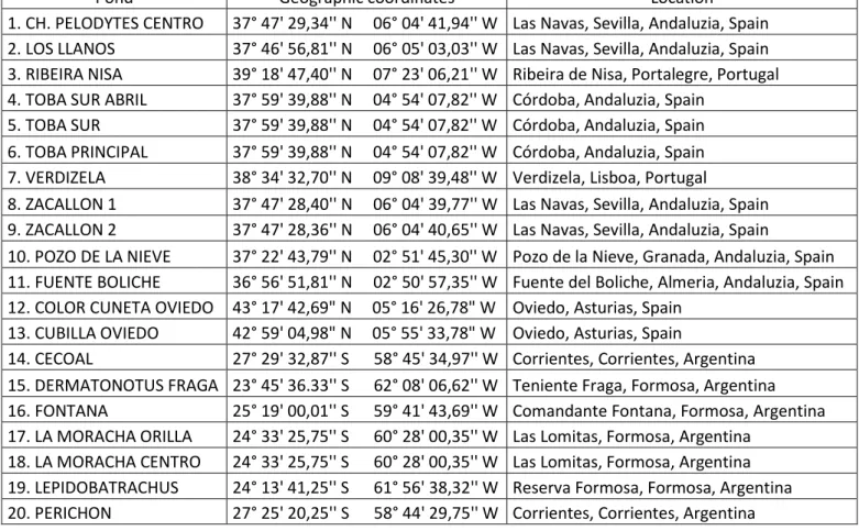
In total, 20 ponds were monitored for both communities, Table 1 (see also Annexe I).
- 12 -
Table 1- Pond location and geographic coordinates.
Pond Geographic coordinates Location
1. CH. PELODYTES CENTRO 37° 47' 29,34'' N 06° 04' 41,94'' W Las Navas, Sevilla, Andaluzia, Spain 2. LOS LLANOS 37° 46' 56,81'' N 06° 05' 03,03'' W Las Navas, Sevilla, Andaluzia, Spain 3. RIBEIRA NISA 39° 18' 47,40'' N 07° 23' 06,21'' W Ribeira de Nisa, Portalegre, Portugal 4. TOBA SUR ABRIL 37° 59' 39,88'' N 04° 54' 07,82'' W Córdoba, Andaluzia, Spain
5. TOBA SUR 37° 59' 39,88'' N 04° 54' 07,82'' W Córdoba, Andaluzia, Spain 6. TOBA PRINCIPAL 37° 59' 39,88'' N 04° 54' 07,82'' W Córdoba, Andaluzia, Spain 7. VERDIZELA 38° 34' 32,70'' N 09° 08' 39,48'' W Verdizela, Lisboa, Portugal
8. ZACALLON 1 37° 47' 28,40'' N 06° 04' 39,77'' W Las Navas, Sevilla, Andaluzia, Spain 9. ZACALLON 2 37° 47' 28,36'' N 06° 04' 40,65'' W Las Navas, Sevilla, Andaluzia, Spain
10. POZO DE LA NIEVE 37° 22' 43,79'' N 02° 51' 45,30'' W Pozo de la Nieve, Granada, Andaluzia, Spain 11. FUENTE BOLICHE 36° 56' 51,81'' N 02° 50' 57,35'' W Fuente del Boliche, Almeria, Andaluzia, Spain 12. COLOR CUNETA OVIEDO 43° 17' 42,69" N 05° 16' 26,78" W Oviedo, Asturias, Spain
13. CUBILLA OVIEDO 42° 59' 04,98" N 05° 55' 33,78" W Oviedo, Asturias, Spain
14. CECOAL 27° 29' 32,87'' S 58° 45' 34,97'' W Corrientes, Corrientes, Argentina 15. DERMATONOTUS FRAGA 23° 45' 36.33'' S 62° 08' 06,62'' W Teniente Fraga, Formosa, Argentina 16. FONTANA 25° 19' 00,01'' S 59° 41' 43,69'' W Comandante Fontana, Formosa, Argentina 17. LA MORACHA ORILLA 24° 33' 25,75'' S 60° 28' 00,35'' W Las Lomitas, Formosa, Argentina
18. LA MORACHA CENTRO 24° 33' 25,75'' S 60° 28' 00,35'' W Las Lomitas, Formosa, Argentina 19. LEPIDOBATRACHUS 24° 13' 41,25'' S 61° 56' 38,32'' W Reserva Formosa, Formosa, Argentina 20. PERICHON 27° 25' 20,25'' S 58° 44' 29,75'' W Corrientes, Corrientes, Argentina
2.2. Comparative evaluation of the upper thermal maxima and Warming Tolerance
Some controversies exist with the employment of different tolerance indices since this diversity inherently reduces the possibility of comparisons among population and species (Berrigan, 2000; Cooper et al., 2008).
To avoid these problems, all upper thermal tolerances were determined by applying the same dynamic method known as CTmax or knockdown temperature (Huey et al., 1992; Lutterschmidt and Hutchison, 1997) which involves increasing the test temperature until an end-point is reached, usually the onset of muscular spasms. Recording of CTmax was done by the same person to reduce any possible bias.
Additionally, some artefacts are associated with CTmax estimates. For instance, basic experimental design such as increased rates of temperature change, cumulative heat shock or very long assays can reduce or inflate the estimates (Czajka and Lee, 1990; Cooper et al., 2008; Chown et al., 2009).
Acclimation also alters heat resistance, often in predictable ways. Higher acclimation temperature induces higher heat resistance (Levins, 1969; Worthen and Haney, 1999; Hoffmann et al., 2003; Navas et al. 2008). In order to avoid bias, acclimation temperature and heating rate used were the same for all studied species from both communities.
- 13 -
A random sample of 15 tadpoles per species was analyzed, with larval developmental stages between 25-39 Gosner’s (Gosner, 1960). Acclimation temperature was set to 20ºC, for a minimum of 4 days. Acclimated individuals were maintained in plastic containers, at a similar larval density, with 12D:12L photoperiod and fed ad libitum.
CTmax was determined by heating tadpoles at a rate of 1°C/min. Tadpoles were individually placed in 400 ml of dechlorinated tap water in a 700 ml glass bowl that was partially submerged within a larger 2000 ml beaker (see figure 8). The water in the larger beaker was heated by an Agimatic‐N (P‐Selecta) magnetic stirrer ensuring a uniform heating of the water in the inner trial beaker. Each trial started at the same temperature as the acclimation temperature. Water temperature was monitored with an electric thermometer (digi‐thermo) (± 0.1°C).
Fig.8- CTmax testing. Overall look of equipment used.
Loss of righting response (LRR) and the onset of spasms (OS) were recorded. OS was defined as the end‐point for CTmax determination following Lutterschmidt and Hutchison (1997) recommendations. Once reached the end‐point, the tadpole was quickly removed from the beaker and placed in cold water in order to recover.
Tested individuals were weighed, to the nearest 0,001g, after excess skin water was gently removed, by placing larvae on a piece of mesh over blotting paper, staged following Gosner’s (1960) and photographed on a scale to estimate body and total lengths.
Statistical analyses of CTmax and WT included analyses of variance, for inter and intraspecific comparisons, and correlations, to determine covariation of traits. Since not all assumptions were met, nonparametric tests were used in most cases (Spearman’s rank R correlation and Kruskal-Wallis ANOVA & Median test). A significance level of α=0,05 was used for all statistical tests. Statistical analyses were
- 14 -
computed using STATISTICA 7.0 software (StatSoft 2000). All data appear as means ± 1 SE or SD.
2.3. Evaluation of thermal sensitivity of locomotor performance and Thermal Safety Margins
Thermal performance curves (TPCs) were obtained in order to estimate thermal sensitivity. TPCs were based on maximal locomotor performance by measuring tadpoles maximal burst swimming speed. Locomotor performance is considered to be a proxy, representing maximum physiological performance, and a critical variable in fleeing from predators (e.g. Feder, 1983; Werner and McPeek, 1994; Watkins 1996).
To determine maximum swimming speed, burst swimming of tadpoles was estimated. Tadpoles were placed on a thermally controlled and opened cross section methacrylate tube and gently prodded with a thin stick to stimulate swimming. Each trial was recorded using a digital camera installed around 2 m above the tube (see figure 9). Tadpoles were acclimated for at least 4 days at 20°C and 9-38 individuals per species were tested (see table 5).
TPCs were defined using 6-7 temperatures within the natural range recorded in the ponds (see Annexe I). For Argentinean species, the test temperatures were 20°, 24°, 28°, 32°, 35° and 38°C and for the Iberian species 10°, 15°, 20°, 24°, 28°, 32° and 35°C. Temperatures were randomized and tadpoles were tested on consecutive days, one temperature per day. Prior to swimming, tadpoles were submitted for half an hour to the test temperature.
Previous analysis with a Chacoan frog community (northern Argentina) revealed that a few species could not tolerate acclimation at 20°C (some Leptodactilids from the Cavicola group, Leptodactylus sp.). This situation matched the thermal profiles measured in the ponds so temperatures lower than 20°C were considered to be out of the natural thermal range for the subtropical Argentinean community. A similar argument was used to select the maximum temperature tested for the Iberian community.
Swimming recordings were analyzed with software Measurement in Motion v3.1 (http://www.motion.com/products/measurement/index.html) that provided tadpole swimming speed at each video recording frame.
After the swimming trials, all tested tadpoles were staged and wet weighed to the nearest 0,001 g. Dorsal and lateral pictures were taken and digitized for morphometric measurements of total length, head‐body length, head‐body height, tail muscle height, total tail height, total tail area, tail muscle area, head‐body width, and tail muscle width (see Dayton et al., 2005) to conduct further morphofunctional analyses, not included in this thesis.
A simple Gaussian model was applied to the data (Angilletta, 2006) in order to estimate optimum temperatures for swimming performance. Statistical analyses of
- 15 -
Topt and TSM were similar to those described for the analyses of CTmax and WT (see Methodology 2.2.).
Fig.9- Swimming performance testing. Overall aspect of equipment assemblage.
2.4. Phylogenetic analyses
The relation of thermal tolerance and sensitivity to habitat temperature was examined within a phylogenetic context to determine the extent to which the observed patterns might derive strictly from phylogenetic relatedness among species (see Stillman and Somero, 2000).
Different phylogenetic techniques may yield different results, especially when the number of species involved is low, since they are based on contrasting evolutionary assumptions (Martins et al. 2002). The use of at least two phylogenetic approaches with different assumptions has been recommended (Martins et al., 2002), in addition to a nonphylogenetic analysis (Garland et al., 1999).
Data were tested for serial independence (TFSI) on continuous characters, to determine whether a trait was significantly associated with its phylogenetic history,
- 16 -
using the software Phylogenetic Independence v2.0 (Abouheif, 1999; see also http://www.biology.mcgill.ca/faculty/abouheif/protocols.html).
Diagnosis was based on a measurement of the autocorrelation of each trait across phylogeny, in the form of a C‐statistic, resulting from similarity between adjacent phylogenetic observations. Topology and associated numerator distribution were randomized 1,000 times and the C‐statistic was calculated for each randomized topology to build the null hypothesis. Observed C‐statistic was compared to the randomized distribution to calculate its level of significance.
If the former analyses revealed that examined traits (CTmax, Topt and Thab) exhibited significant phylogenetic autocorrelation, the coevolution of all traits will require a correction for phylogeny since data is not independent. In order to avoid this bias, correlations between traits were obtained using the method of phylogenetically independent contrasts (PIC) as described by Felsenstein (1985), with PDTREE module (PDAP package by Midford et al., 2003) for Mesquite (v. 2.6) software (Maddison and Maddison, 2009).
PIC is a method of correcting for phylogeny. It requires that both the tree topology and the branch lengths are known, and that characters are allowed to be modelled by Brownian motion on a linear scale. Given these conditions, the phylogeny specifies a set of contrasts among species, contrasts that are statistically independent and can be used in regression or correlation studies (Felsenstein, 1985).
Using independent contrasts, PDTREE also allows the estimation of ancestral states (values at internal nodes or at any point along a branch) and their standard errors (Garland et al., 1999). In most cases, PIC is mathematically and statistically equivalent to generalized least-squares (GLS) models (Garland et al., 2005).
Previous works have used similar analysis to evaluate evolutionary trends amongst traits in amphibians (see Gvozdik and van Damme, 2008, for an example with European newts).
For these analyses, three phylogenetic trees were constructed based on Frost et al (2006), including only the studied species: one for each community and one combining all species from both communities (see Annexe II). All branch lengths were set equal to one.
- 17 -
3. RESULTS
3.1. Monitoring environmental temperatures
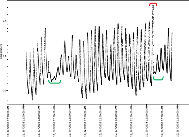
Thermal profiles of the ponds were obtained from the dataloggers placed in the water. Figure 10 shows the output of a selected datalogger. By examining the output, it is possible to identify periods of stormy and clouded days associated with rains (marked in green) and periods where the pond was entirely dry (marked in red), with the sensor presumably measuring air temperature. This information was taken into account while estimating maximum, average and minimum temperatures for the ponds.
Fig.10- Temporary pond at Comandante Fontana (Formosa province, Argentina, 25° 19' 00,01'' S, 59° 41' 43,69'' W) depth range (max‐min) between 25‐0 cm depth, 18th November‐26th December 2008.
Table in Annexe I provides data on all the ponds monitored and their water temperatures.
Figure 11 shows both shoreline and maximum depth water temperatures for a selected pond, during three consecutive days. Two conclusions can be derived from these observations: first, during the coldest time of the day there is no apparent difference between the two sites while during the warmest there is a clear thermal divergence, with higher values at the shoreline; second, both sites cool at the same rate but differ on their heating rate.
- 18 -
This situation has several biological implications. Tadpoles cannot escape the minimum temperature because the pond’s water is thermally homogeneous. During the warmest part of the day, tadpoles can behaviourally thermoregulate selecting amongst a range of temperatures, thus avoiding, into some extent, somewhat undesirable and dangerously high temperatures.
There is a significant difference between the two communities regarding both their Average (Kruskal-Wallis test: H1,20=13,00; p=0,0003; N=20) and Maximum
Temperature (ANOVA: F1,20=13,79032; p=0,000072; N=20) with higher temperatures
occurring in the subtropical community (maximum: 38,24°C, SD=2,85°C; average: 26,66°C, SD=1,5°C). In the temperate Iberian community, habitat temperatures were generally cooler (maximum: 28,28°C, SD=4,67°C; average: 13,60°C, SD=3,07°C).
Fig.11- The same pond as in figure 3 but with two different temperature records: at maximum depth (25 cm depth, blue) and at the shore (3 cm depth, red) between 18th‐21st November 2008.
For each species, average and maximum temperatures were scored for all ponds monitored where each particular species was collected (Table 2). These values were used in the calculation of species thermal safety margins and warming tolerance, respectively.
- 19 -
Table 2- Average and maximum temperatures per species and per community (Iberian Peninsula (IP) and Argentina (ARG).
Species Community Average Temperature Maximum Temperature
Pond T ºC Pond T ºC
A. cisternasii IP Toba Sur Abril 10,64 Toba Sur Abril 24,16
A. dickhilleni IP Fuente Boliche 12,52 Fuente Boliche 25,13
E. calamita IP LosLlanos 14,58 Toba Sur 34,16
P. cultripes IP Zacallon 1 10,88 Ch.Pelodytes 35,54
P. ibericus IP Toba Principal 18,11 Ch.Pelodytes 35,54
H. arborea IP Verdizela 21,06 Verdizela 31,37
H. meridionalis IP Toba Principal 18,11 Toba Sur 34,16
R. iberica IP Ribeira Nisa 14,02 Ribeira Nisa 29,05
R. temporaria IP Cubilla Oviedo 12,21 Cubilla Oviedo 24,47
E. bicolor ARG CECOAL 24,17 CECOAL 34,16
H. raniceps ARG Perichon 25,38 Perichon 38,21
L. bufonius ARG Fontana 27,32 Fontana 40,09
L. latinasus ARG La MorachaOrilla 27,43 La MorachaOrilla 38,73
L. limellum ARG Perichon 25,38 Perichon 38,21
P. albonotatus ARG Fontana 27,32 Fontana 40,09
P. paradoxa ARG Perichon 25,38 Perichon 38,21
S. acuminatus ARG Perichon 25,38 Perichon 38,21
S. nasicus ARG Perichon 25,38 Perichon 38,21
T. venulosus ARG La MorachaOrilla 27,43 La MorachaOrilla 38,73
To estimate Warming Tolerance, maximum temperature was selected instead of average temperature because it better reflects the risk that high environmental temperatures represent to the tadpoles (in disagreement with Deutsch et al., 2008 who used mean annual temperature for calculating both Warming Tolerance and Thermal Safety Margins). For instance, if habitat temperature rises above CTmax value, even if it happens only once, it will be fatal for the species survival. Therefore it is considered to be more realistic to estimate warming tolerance using the highest habitat temperature found because it represents the most extreme situation that the species was exposed to during this monitoring period.
To estimate Thermal Safety Margins, average temperature of the pound was used. It is argued that, when comparing optimal temperatures with habitat temperatures, it seems more realistic to use average temperature of the pond rather than the highest temperature recorded because it represents, to some extent, the temperature tadpoles where exposed to during all their larval phase. Maximum temperature can represent a temperature tadpoles were only occasionally exposed to during their larval stage.
- 20 -
3.2. Upper thermal maxima and Warming Tolerance
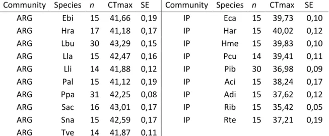
In total, 19 species were tested for CTmax, 10 from the Argentinean community and 9 from the Iberian Peninsula. Results are shown in Table 3.
Table 3- Community of origin, sample size, average CTmax response and respective SE of all species studied.
Community Species n CTmax SE Community Species n CTmax SE
ARG Ebi 15 41,66 0,19 IP Eca 15 39,73 0,10
ARG Hra 17 41,18 0,17 IP Har 15 40,02 0,12
ARG Lbu 30 43,29 0,15 IP Hme 15 39,83 0,10
ARG Lla 15 42,47 0,16 IP Pcu 14 39,41 0,11
ARG Lli 14 41,88 0,12 IP Pib 30 36,98 0,09
ARG Pal 15 41,12 0,19 IP Aci 15 38,24 0,17
ARG Ppa 31 42,25 0,08 IP Adi 15 37,62 0,12
ARG Sac 16 43,01 0,17 IP Rib 15 35,42 0,05
ARG Sna 15 42,59 0,17 IP Rte 15 37,21 0,19
ARG Tve 14 41,87 0,11
ARG: Argentina community, IP: Iberian Peninsula community. Species - Ebi: Elaschistocleis bicolor; Hra:
Hypsiboas raniceps; Lbu: Leptodactylus bufonius; Lla: Leptodactylus latinasus; Lli: Pseudis limellum; Pal: Physalaemus albonotatus; Ppa: Pseudis paradoxa; Sac: Scinax acuminatus; Sna: Scinax nasicus; Tve: Trachycephalus venulosus; Aci: Alytes cisternasii; Adi: Alytes dickhilleni; Eca: Epidalea calamita; Har: Hyla arborea; Hme: Hyla meridionalis; Pcu: Pelobates cultripes; Pib: Pelodytes ibericus; Rib: Rana iberica; Rte: Rana temporaria.Both CTmax and SE were expressed in :C.
Species differ significantly in CTmax value within both the Iberian community (Kruskal-Wallis test: H8,149=126,8174; p<0,001) and the Argentinean community
(F9,171)=25,529, p<0,0001), see also Annexe III.
Using the mean CTmax for each species (Table 3), a significant difference between the two communities was found (Kruskal-Wallis test: H1,19=13,500; p=0,0002;
N=19). Argentinean community (42,13°C, SD=0,73°C) has a value of CTmax almost 4ºC higher than the Iberian community (38,27°C, SD=1,59°C), as shown in figure 12. Nevertheless, the Iberian community displayed more variation in CTmax (Levene's test: F1,17=6,8906; p=0,0177; N=19).
- 21 -
Comparing Communities - CTmax
Species C T m a x Iberian Peninsula Argentina A. ci st e rn a si i A. d ickh il le n i E. ca la m it a P. cu lt ri p e s P. i b e ri cu s H . a rb o re a H . m e ri d io n a li s R . ib e ri ca R . te m p o ra ri a E. b ico lo r H . ra n ice p s L . b u fo n iu s L . la ti n a su s L . li m e ll u m P. a lb o n o ta tu s P. p a ra d o xa S. a cu m in a tu s S. n a si cu s T . ve n u lo su s 35 36 37 38 39 40 41 42 43 44
Fig.12– Estimated mean value of CTmax (solid lines) and SD (dotted lines) for each community.
Warming Tolerance is shown in Table 4. There is a significant difference between the two communities in WT (Kruskal-Wallis test: H1,19=5,6067; p=0,0179;
N=19; Argentina: 3,85 :C, SD=1,64:C; Iberian Peninsula: 7,88 :C, SD=4,39:C). Table 4- Warming Tolerance (WT) for all species from both communities.
Iberian Peninsula Argentina
Species WT Species WT A. cisternasii 14,08 E. bicolor 7,50 A. dickhilleni 12,49 H. raniceps 2,97 E. calamita 5,57 L. bufonius 3,21 P. cultripes 3,87 L. latinasus 3,75 P. ibericus 1,44 L. limellum 3,67 H. arborea 8,65 P. albonotatus 1,04 H. meridionalis 5,67 P. paradoxa 4,04 R. iberica 6,37 S. acuminatus 4,80 R. temporaria 12,74 S. nasicus 4,38 T. venulosus 3,14
- 22 -
Iberian species have higher warming tolerance (figure 13), and continue to show more variation than the Argentinean community (Levene's test: F1,17=11,6626;
p=0,003299; N=19).
Interestingly, species from Argentinean community although having higher values of CTmax generally have lower warming tolerance. There is a slight negative correlation, although not significant, between CTmax and WT (Spearman’s rs=-0,379;
p=0,1096).
Comparing Communities - Warming Tolerance
Species W T Ab s M a x Iberian Peninsula Argentina A. ci st e rn a si i A. d ickh il le n i E. ca la m it a P. cu lt ri p e s P. i b e ri cu s H . a rb o re a H . m e ri d io n a li s R . ib e ri ca R . te m p o ra ri a E. b ico lo r H . ra n ice p s L . b u fo n iu s L . la ti n a su s L . li m e ll u m P. a lb o n o ta tu s P. p a ra d o xa S. a cu m in a tu s S. n a si cu s T . ve n u lo su s 0 2 4 6 8 10 12 14 16
Fig.13– Estimated mean value of Warming Tolerance (WT) (solid lines) and SD (dotted lines) for each community.
There is a strong correlation between maximum habitat temperature and CTmax (Spearman’s rs=0,758; p=0,000169), as shown in figure 14. This implies that
species exposed to higher temperatures also have higher CTmax values. When considering both communities separately, no significant correlations were found (Iberian Peninsula: Spearman’s rs=0,21; p=0,5874 and Argentina: Spearman’s rs=0,098;
- 23 -
Correlation between CTmax and Thabitat (Abs Max) CTmax = 28,4949+0,3418*Abs Max; 0,95 Conf.Int.
Correlation: Spearman R=0,758; p=0,000169 Adi Aci Eca Pcu Pib Har Hme Rib Rte Ebi Hra Lbu Lla Lli Pal Ppa Sac Sna Tve 22 24 26 28 30 32 34 36 38 40 42 Abs Max 35 36 37 38 39 40 41 42 43 44 C T ma x
Fig.14– Correlation between maximum habitat temperature (Abs Max) and CTmax. Green lines represent 95% confidence intervals. Argentinean community in red and Iberian community in blue. Species - Ebi: Elaschistocleis bicolor; Hra: Hypsiboas raniceps; Lbu: Leptodactylus bufonius; Lla:
Leptodactylus latinasus; Lli: Pseudis limellum; Pal: Physalaemus albonotatus; Ppa: Pseudis paradoxa; Sac: Scinax acuminatus; Sna: Scinax nasicus; Tve: Trachycephalus venulosus; Aci: Alytes cisternasii; Adi: Alytes dickhilleni; Eca: Epidalea calamita; Har: Hyla arborea; Hme: Hyla meridionalis; Pcu: Pelobates cultripes;
Pib: Pelodytes ibericus; Rib: Rana iberica; Rte: Rana temporaria.
Regarding CTmax, a phylogenetic signal was obtained for the combined tree of the two communities (C=0,541211; p=0,011) but phylogenetic autocorrelations were not found when analysing either the Iberian community (C=0,170625; p=0,12) or Argentinean community (C=0,089523; p=0,3730) separately. For maximum habitat temperature, a phylogenetic signal was obtained for all three combinations (Argentina: C=0,144591; p=0,033; Iberian Peninsula: C=0,454365; p=0,033 and combined communities: C=0,69786; p=0,001).
This suggests that the tip correlation between CTmax and maximum habitat temperature may be affected by phylogenetic history and therefore, the use of phylogenetic independent contrasts is justified (Rheindt et al., 2004).
After correcting for phylogeny, in none of the three possible cases (Iberian community, Argentinean community and the combination of both) a correlation was found. However, the p-value for the combined tree was 0,1097, close to statistical significance (figure 15).
- 24 -
Fig.15– Plot of contrasts vs. positivized contrasts for combined tree for both Argentina and Iberian Peninsula communities (CTmax, Thabitat). Number of contrasts: 18; Pearson Product-Moment Correlation Coefficient: 0,379; Two tailed p-value: 0,10977; Regression lines through origin: Black is ordinary least squares (OLS), Green is major axis (MA) and Red is reduced major axis.
3.3. Thermal sensitivity and Thermal Safety Margins
In total, 18 species were tested for thermal sensitivity, 9 from the Argentinean community and 9 from the Iberian Peninsula. Results are shown in Table 5.
Table 5- Community origin, sample size, estimated optimum temperature (Opt) and temperature of highest performance (T) of all species studied.
Community Species n Opt T Community Species n Opt T
ARG Ebi 19 31,02 28 IP Eca 20 35,61 35
ARG Hra 18 36,14 35 IP Har 14 36,09 35
ARG LEP 9 38,04 35 IP Hme 15 37,64 35
ARG Lli 16 33,09 28 IP Pcu 20 37,98 35
ARG Pal 18 36,17 38 IP Pib 38 26,93 24
ARG Ppa 21 30,56 28 IP Aci 20 22,82 24
ARG Sac 19 35,81 38 IP Adi 19 23,00 24
ARG Sna 20 35,03 38 IP Rib 14 26,64 28
ARG Tve 20 39,09 38 IP Rte 14 23,70 24
ARG: Argentina community, IP: Iberian Peninsula community. Species - Ebi: Elaschistocleis bicolor; Hra:
Hypsiboas raniceps; LEP: Leptodactylus sp.; Lli: Pseudis limellum; Pal: Physalaemus albonotatus; Ppa: Pseudis paradoxa; Sac: Scinax acuminatus; Sna: Scinax nasicus; Tve: Trachycephalus venulosus; Aci: Alytes cisternasii; Adi: Alytes dickhilleni; Eca: Epidalea calamita; Har: Hyla arborea; Hme: Hyla meridionalis; Pcu: Pelobates cultripes; Pib: Pelodytes ibericus; Rib: Rana iberica; Rte: Rana temporaria.
- 25 -
The symbol “T” shown in Table 5 refers to the treatment temperature at which tadpoles had the best overall swimming performance and Topt is the estimated optimum temperature (see also figure 16 and Annexe IV).
Alytes cisternasii
Vertical bars denote 0,95 confidence intervals
10 15 20 24 28 32 Temperature (ºC) 0,30 0,35 0,40 0,45 0,50 0,55 0,60 0,65 0,70 0,75 0,80 0,85 0,90 Sp e e d ( m/ s )
Fig.16–Swimming speed of Alytes cisternasii (blue), by treatment temperature. Best overall swimming performance (red circle) and estimated Optimum temperature and performance curve (green circle and line).
Optimum temperatures were higher in the Argentinean community, although not statistically different from those of the Iberian Peninsula community (Kruskal-Wallis test: H1,18=2,387914; p=0,1223; N=18; Argentina: 34,99:C, SD=2,93:C; Iberian
Peninsula: 30,05:C, SD=6,63:C), as shown in figure 17. Variance in optimum temperature was higher for the Iberian community (Levene’s test: F1,16=22,12609;
p=0,000239; N=18).
If the comparison is made using T temperature (from Table 5), a significant difference is found (Kruskal-Wallis test: H=4,421337; p=0,0355; N=18) which confirms the tendency found in the previous test.
Interestingly, Iberian species Topt values can be differentiated into two groups: a cool Topt group that encompases Alytes cisternasii, Alytes dickhilleni, Pelodytes
ibericus, Rana iberica and Rana temporaria; and a warm Topt group, containing Epidalea calamita, Pelobates cultripes, Hyla arborea and Hyla meridionalis.
Covariate means: Weight: 0,885 g
- 26 -
These two groups differ significantly in their optimum temperature (Kruskal-Wallis test: H1,9=6,000; p=0,0143; N=9). The cool group also differs significantly from
the Argentinean community (Kruskal-Wallis test: H1,14=9,000; p=0,0027; N=14).
Average value of the warm group (36,82°C, SD=1,16°C) did not differ from the one found for the Argentinean community (Kruskal-Wallis test: H1,13=0,5952; p=0,4404;
N=13).
Comparing communities - Optimum Temperature
Species O p t Argentina Iberian Peninsula A. ci st e rn a si i A. d ickh il le n i E. ca la m it a P. cu lt ri p e s P. i b e ri cu s H . a rb o re a H . m e ri d io n a li s R . ib e ri ca R . te m p o ra ri a E. b ico lo r H . ra n ice p s L EP sp . L . li m e ll u m P. a lb o n o ta tu s P. p a ra d o xa S. a cu m in a tu s S. n a si cu s T . ve n u lo su s 22 24 26 28 30 32 34 36 38 40
Fig.17– Estimated Optimum Temperature (Opt) (solid lines) and SD (dotted lines) for each community. Thermal Safety Margins appears in Table 6. There is a significant difference between the two communities (F1,18=11,2286; p=0,0041; N=18), with the Iberian
community having higher value of TSM (13,51 :C; SD=3,34:C) than that found for Argentina species (9,09:C; SD=2,13:C), as shown in figure 18.
Similar to CTmax and WT, the species from Argentinean community, although having higher values of optimum temperature, generally have narrower thermal safety margins. There is no significant correlation between Optimum temperature (Topt) and TSM (Spearman’s rs=0,292; p=0,2396).
- 27 -
Table 6- Thermal Safety Margins (TSM) for all species from both communities.
Iberian Peninsula Argentina
Species TSM Species TSM A. cisternasii 12,18 E. bicolor 6,85 A. dickhilleni 10,48 H. raniceps 10,76 E. calamita 14,55 Leptodactylus sp. 10,72 P. cultripes 16,93 L. limellum 7,71 P. ibericus 8,82 P. albonotatus 8,85 H. arborea 15,03 P. paradoxa 5,18 H. meridionalis 19,53 S. acuminatus 10,43 R. iberica 12,62 S. nasicus 9,65 R. temporaria 11,49 T. venulosus 11,66
Comparing communities - Thermal Safety Margins (TSM)
Species T SM (ca lcu la te d w it h O p t) Community: ARG Community: IP A. ci st e rn a si i A. d ickh il le n i E. ca la m it a P. cu lt ri p e s P. i b e ri cu s H . a rb o re a H . m e ri d io n a li s R . ib e ri ca R . te m p o ra ri a E. b ico lo r H . ra n ice p s L EP sp . L . li m e ll u m P. a lb o n o ta tu s P. p a ra d o xa S. a cu m in a tu s S. n a si cu s T . ve n u lo su s 4 6 8 10 12 14 16 18 20 22
Fig.18– Thermal Safety Margins (TSM) (solid lines) and SD (dotted lines) for each community, using estimated optimum temperature.
Average habitat temperature and optimum temperature exhibit a strong correlation (Spearman’s rs=0,6977; p=0,001286, figure 19). This suggests that species
exposed to higher average temperatures have a higher optimum temperature. Considering both communities separately, there was also a significant correlation (Iberian Peninsula: Spearman’s rs=0,857; p=0,00314 and Argentina: Spearman’s rs