Parallel Switching Regulatory Control of Iron Ore Flowrate from Multiple Feeders with Time Delay

(1)

JOURNAL OF APPLIED INSTRUMENTATION AND CONTROL - V.06. N.1 1 ‘

Abstract — The suitable performance of an industrial process needs regulatory control loops to adjust the main process variables to their specified reference values (set-points), and to compensate for eventual load disturbances on the process. Regulatory control is fundamentally used in the industry for stabilizing process variables, and it is generally implemented through the plantwide control system architecture (SCADA or DCS). The absence or inefficiency of control in an industrial process always implies in losses of productivity, so that regulatory control is a key issue for improving process performance. In this context, this article presents the development and implementation of a control strategy for regulating the output mass flow (in t/h) of a Crushing facility in the Carajás Iron Ore Processing Plant I. The facility has eight feeders in parallel, and the goal is to control them so that their resulting combined output flow matches a specified production set-point (in t/h). The article first explains the process, the control problem, and the transfer function model of the process. Subsequently, one is presented the control strategy, which is based on a switching between a constant and a PI control action. The suitability of the strategy was investigated through computational simulations. Finally, the results and conclusions are discussed.

Index Terms— mass flowrate control, regulatory control, PID control, programmable logic controller, supervisory control and data acquisition, switching control.

I. INTRODUCTION

INERAL processing plants are formed by several processing facilities, involving stages of crushing, screening, classifying, grinding, hydrocycloning, and filtration, among others. The Carajás Iron Ore Processing Plant I, that belongs to VALE, had been responsible for an 83 million tons annual production (year 2005), mostly destined to exportation, having as main customers: Japan, Germany, China, Korea, and France. Its high installed capacity and high daily production goals, of about 260,000 tons/day, has demanded better practices

of industrial operation, maintenance and automation. The Automation Department is responsible for the definition, implantation, and quality assurance of control strategies to improve productivity and reduce wastefulness in the plants by the use of automation resources. In this scenario, this work addresses the problem of improving the production control of a Crushing facility of the referred plant.

II. ORE CRUSHING FACILITY

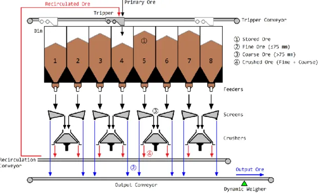
The Secondary Crushing facility of the Carajás Iron ore Plant [1;2;3] is shown in Figures 1 and 2. It’s formed by a large bin with eight cells, each of them having a feeder and a screen, besides four crushers, a recirculation conveyor, and an output conveyor. This facility receives a near raw ore from Primary Crushing facilities located far inside the mine, and its function is to reduce such ore to a maximum output size of 75 mm. The primary ore comes through an input conveyor assembled to a tripper car which discharges the ore inside the bin. The tripper moves forward and backward along the bin to spread the ore in the cells. Each cell has a nominal volumetric capacity of 1,040 m3_{, corresponding to 5,200 t, in average, depending on the} density, moisture content, and size distribution of the ore. Figure 3 shows one of the feeders under the bin. The feeders discharge the ore on their respective screens, which separate the fine ore (< 75 mm) from the coarse ore (≥ 75 mm). This 75-mm separation size is defined by the hole size of the screens meshes, and is termed as “cut-off size”.

The primary ore contains, in average, 90% of fine and 10% of gross material. The gross ore, which doesn’t pass through the screens meshes, falls in the crushers to be reduced in size, and then comes back to the bin through the recirculation conveyor, shown in Figure 4. The fine ore, which pass through the screens meshes, forms the output ore of the Crushing facility, and follows to a subsequent facility through the output conveyor, shown in Figure 5. Each feeder is driven by an induction motor powered by a variable frequency driver (VFD) to adjust its speed, and hence the mass flowrate delivered by the feeder.

Sidney A. A. Viana

____________________________________________________________________________

Parallel Switching Regulatory Control

of Iron Ore Flowrate from Multiple

with Time Delay

M

______________________________________________________________ S. A. A. Viana is an Specialist Automation & Control Systems Engineer, and Senior Member of the IEEE – The Institute of Electrical and Electronics Engineers. He is currently with the Advanced Analytics & Machine Learning Team, at VALE’s Centre of Excellence, Belo Horizonte, MG, Brazil (e-mail: [email protected]).).

(2)

Fig. 1. Illustration of the Secondary Crushing Facility of the Carajás Iron ore processing Plant.

Fig. 2. The Secondary Crushing Facility.

Fig. 3. One of the feeders under the bin.

Fig. 4. Recirculation conveyor.

(3)

The total output mass flowrate of the Secondary Crushing facility is the main process variable. It’s measured by a dynamic weigher (belt scale) assembled in the output conveyor. The output flowrate must follow the production set-point defined by Plant Operators, according to the production demand. The output flow is subject to the following operational constraints:

1) Capacity of the production lines, vL(max)

Each pair feeder/screen defines a production line of the Crushing facility. The output flow of a line is given by the ore that pass down through its respective screen. Each feeder is calibrated so that the maximum flow vL(max) of the line is 3,000

t/h. The ore that pass down through the screen is about 90% of the total ore delivered by the feeder, so that the maximum flow

vF(max) given by the feeder is about 3,000/0.9 = 3,300 t/h. t/h 300 , 3 (max) F v (1) t/h 000 , 3 (max) L v (2)

2) Number of feeders in operation, N

The output flow of the Crushing facility is the sum of the individual flows of the operating lines, and it is therefore limited by the maximum flow vL(max) of the lines and by the

number N of feeders in operation.

(max) (max) N.vL

y  (3)

Thus, for example, the maximum total output flow with four feeders in operation is about 12,000 t/h.

3) Time-delay, 

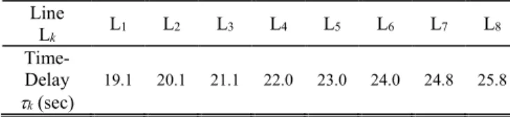
Each feeder (actuator) is located at a specific distance from the dynamic weigher (sensor), and therefore there are specific time-delays for each line, which are indicated in Table I, in Section III.

III. THE CONTROL PROBLEM

The control problem related to the feeders is described in the following.

A. Performance with no automatic control

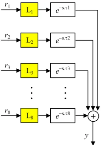
According to the process description in Section II, the block diagram of the ore production process of the Secondary Crushing facility, is shown in Figure 6, where Lk represents the k-th line (k = 1, 2, ..., 8); rk is the input of the k-th feeder (0% to 100%); k is the time-delay for feeder k; sp is the production

set-point; and y is the total output flow of the facility, measured by the dynamic weigher.

In terms of operation, the feeders inputs rk must be adjusted

so that the output flowrate y can be stabilized around the production set-point sp. In the original operation procedure, with no automatic control, the inputs rk were manually adjusted

by Plant Operators at the Control Room, through the Supervisory System. Under this open loop operation, the values of rk could not be changed dynamically to compensate for

variations in the output flowrate due to changes in the physical

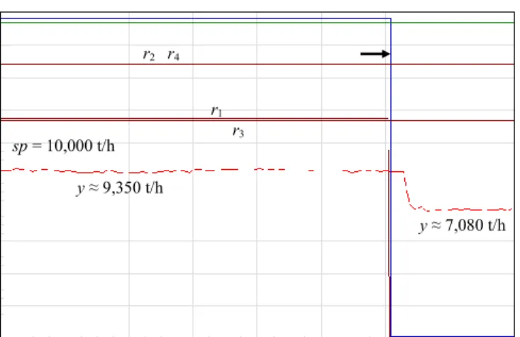
properties of the ore (density, moisture content, and size distribution) or due to stops of production lines. The operators had to continuously pay attention to the process through the Supervisory System to identify the need for compensations. This manual operation caused high workloads for the operators. An example of open loop operation of the Crushing facility is shown in Figure 7, for a 15-minutes period. The Plant was operating with feeders 1 to 4 with the following individual set-points rk: r1 = 81.17%, r2 = 100%, r3 = 80.18%, and r4 = 100%. The lines at the top of the graph indicate the operating status of the feeders (1: operating; 0: stopped). Those status lines are in slightly different scales in the graph to avoid overlapping, and they are also sequentially ordered for each feeder, so that the line at the uppermost position relates to feeder 1. The production set-point sp and the output flowrate y are in the same scale. The output flowrate was initially stabilized at about y = 9,350 t/h, however, bellow the production set-point sp = 10,000 t/h, due to the open loop operation. At the instant indicated by the arrow, the feeder 1 stopped operating and led the output flowrate to fall to y = 7,080 t/h, with no further compensation by the remaining operating feeders. Similar situation should occur in the case of starting any feeder with the output flowrate already stabilized at set-point sp: the operators must have to manually reduce the individual set-points rk of the operating

feeders before starting an additional feeder.

Furthermore, to assure overload protection of the output conveyor, the production set-point sp was also used as a

protective on-off limiter for the output flowrate y: whenever y

exceeds sp for 6 seconds, one of the operating feeders would be stopped to force y to decrease below sp. As an example, Figure 8 shows the set-point sp, the output flowrate y, and the operating status of the feeders for a 50-minutes period. The six arrows indicate stoppings of feeder 2 by the protective on-off limiter. Such stoppings became frequent in open loop operation, leading to losses of production.

Fig. 6. Block diagram for mass flowrate in the Secondary Crushing Facility. r1 y r2 r3 r8 L1 es.1 L2 es.2 L3 es.3 L8 es.8       +

(4)

B. Definition of the need for automatic control

As explained before, the open loop operation of the Crushing facility with a protective on-off limiter would never allow an effective regulation of the output flowrate, and led to frequent feeder stoppings, with consequent losses of production. Besides this ineffective operation scenario, the need for automatic control of the output flowrate was also related to three operational aspects of the facility:

1) Variability of mass flowrates

A feeder operating at a fixed speed gives a relatively uniform volumetric flowrate of ore. Nevertheless, the mass flowrate depends not only on the volumetric flowrate, but also on the density, moisture content, and size distribution of the ore. Moisture content and density variations cannot be controlled and cannot be eliminated from the process, so that the mass flowrate delivered by a feeder operating at a fixed speed will always have a variability, which can be considered as process noise. This variability will be naturally reflected on the total output flowrate y of the facility, and it may lead y to exceed the set-point sp causing actuation of the protective on-off limiter of the output conveyor, even if y is stabilized slightly below sp.

2) Productivity losses due to feeder stoppings

In case of stopping of a production line, the total output flowrate y will fall and stay at a lower value if there is no further increase of the individual inputs rk of the remaining

operating feeders. This condition leads to losses of production, as exemplified in Figure 7.

3) Operational safety on feeder startings

In case of starting of any feeder, the total output flowrate y will naturally increase. However, depending on the current set-point sp, the total output flow y may exceed the value of

sp causing actuation of the protective on-off limiter of the

output conveyor. Hence, the operators must decrease manually the individual inputs rk of the operating feeders

before starting any additional feeder.

In short, the Secondary Crushing facility had losses of production due to its open loop operation with the feeders set-points being determined manually by the operators, without feedback of the total output flowrate, and disregarding the effects of starting or stopping feeders. This ineffective operational scenario motivated the implementation of a regulatory control strategy for the feeders, in order to reduce the production losses resulting from the open loop operation.

C. The Process Model

By observing in loco the ore flow of the production lines, and analyzing recorded flowrate data measured by the dynamic weigher, one was concluded that the lines could be represented by a first-order plus time-delay (FOPDT) transfer function model [7;8]. The first-order model was found suitable because the feeder’s driver system is inherently overdamped. In addition, several flowrate response curves from all the lines were analyzed. For all the lines, the DC gain was found near unity, K ≈ 1, and the time constant was evaluated as T ≈ 6,3 s. Thus, the dynamic model considered for each production line was:   s s _e s e Ts K s G       1 3 . 6 1 1 ) ( (4)

The time-delays of the production lines were evaluated from recorded flow data, resulting in the approximate values shown in Table I. Notice that the time-delays are significantly higher than the time constant. The process model in (4) was used in the designing and evaluation of the automatic control strategy.

IV. THE CONTROL STRATEGY The control strategy is described in the following.

A. Switching Regulatory Control for a Time-Delayed Process

For a process with high time-delay controlled by a proportional-integral (PI) controller, the integral gain of the controller should be sufficiently low to avoid excessive overshoots and oscillations in the process output. Nevertheless, lower gains may lead to slower outputs with higher settling times. The strategy used to deal with this Fig. 7. Open loop performance of the Secondary Crushing Facility.

Fig. 8. Feeder 2 stoppings due to actuation of the protective on-off limiter.

sp = 10,000 t/h y ≈ 9,350 t/h r1 r3 r2 r4 y ≈ 7,080 t/h sp y

(5)

trade-off was a switching control between a constant control action and a PI control action. The constant control action should be defined by the steady state relationship between the process input (manipulated variable or control signal) and the process output (controlled variable or process output). The idea is to give a constant initial control action to force a fast initial response of the process output, and then turn to the PI control action to achieve the final regulation of the output.

For better understanding, the strategy will be exemplified regarding the control block in Figure 9, which represents a single line of the Crushing facility. The transfer function

G(s) is given by equation (4), and C(s) is a PI controller

tuned in such a way to avoid excessive overshoot in the output. The method used to tune the controller parameters was the Root Locus Method [7,8]. The resulting controller gains were: KP = 0.1, and KI = 0.018. Figure 10 shows the

performance of the system for a set-point r = 3,000 t/h. The PI control signal u starts increasing fastly due to the high actuating error caused by the time-delay of the output. The settling time is about 118 s. Now, in an attempt to make the output even faster, the integral gain of the controller was increased to KI = 0.025, resulting in an output with higher

overshoot, as shown in Figure 11. The higher value of KI

amplifies the integral component of the control signal, leading the output to increase significantly beyond its steady state value. Clearly, the time-delay imposes a performance limitation: it’s not possible to make the output faster without increasing the overshoot significantly.

To implement the switching control, the steady state relationship between the control signal u and the output y must be firstly determined. For the system in Figure 9, it can be shown that this steady state relationship has the form: uss

= (1/K).yss = α.yss. Assuming that the controller C(s) should

stabilize the process output at the set-point r, thus yss ≈ r,

and therefore uss = α.r. For the system in Figure 9, the output

stabilizes in yss = r = 3,000 t/h, meaning a steady state

relationship uss = (3,000/3,000).yss ≈ (1.0).r, which is valid

for any value of r. The steady state relationship defines the control signal that stabilizes the controlled variable in the set-point r. Therefore, whenever the set-point changes to a new value rn, the process input will be momentarily

switched to a constant control action uf = β.uss (0 ≤ β ≤ 1)

for a specific “forcing time” Tu in order to force a fast initial

transitory output. When the forcing time ends, the process input is switched to the PI control signal to achieve the final regulation of the output. During the forcing time, by which the constant control action un is acting on the process input,

the PI controller stays in “manual mode” and its output is not changed by the error, but it follows the constant control signal to achieve “bumpless transfer” [7;8] when the process input is switched to the PI controller. β and Tu are design

parameters which can be properly chosen with the use of simulations on the process model shown in Figure 9. The performance provided by the switching control is shown in Figure 12. The constant control signal was chosen as 80% of the value uss needed to stabilize the process

variable at the set-point r, that is, un = uf = β.uss = 0.8uss =

0.8(1.0)r = 2,400. This constant control signal actuates on the process input during a forcing time Tu = 20 s, by the end

of which the process input is switched to the PI controller, which then performs the final regulation of the output. Here,

sp u

y

TABLEI

TIME-DELAYS OF THE PRODUCTION LINES FROM THE CRUSHING FACILITY

Line Lk L1 L2 L3 L4 L5 L6 L7 L8 Time-Delay k (sec) 19.1 20.1 21.1 22.0 23.0 24.0 24.8 25.8

Fig. 9. Block diagram for closed loop control of a single production line.

Fig. 10. Closed loop performance with tuned controller.

G(s)

e

s.

C(s)

+ 

r

u

y

Fig. 11. Closed loop performance with increased integral gain.

Fig. 12. Closed loop performance with switching control.

sp u

(6)

the gains of the PI controller were KP = 0.01 and KI = 0.014,

obtained using the Root Locus Method. Notice that these gain values are lower than that used in the simulation of Figure 10 because the final regulation with the switching control does not require an “aggressive” actuation of the PI controller, due to the strong initial action of the constant control signal un = uf.

The parameter β defines the intensity of the constant control action uf, and its increase makes the output y faster. The increase

of the forcing time Tu tends to stabilize the output closer to the

value β.r. Several simulations performed with different values for β and Tu suggested two basic rules to choose such

parameters:

 Tu should be chosen between 80% and 90% of the

time-delay  of the process.

 β should be chosen between 0.8 and 1.0, to achieve small overshoots in the process output. If a high overshoot results, one can reduce the gains of the controller, reduce

Tu, or reduce β.

Since the main goal of work was to solve a practical control problem in an industrial context, it does not intend to formulate analytical criterions and formal equations for calculating β and

Tu. This is left as issue for further works.

B. Parallel Switching Regulatory Control of Mass Flowrate

The switching control strategy explained in Section IV was applied in parallel to the eight feeders of the Crushing facility. The block diagram of the control system is shown in Figure 13. As the individual output flowrate of the feeders are not directly measured, the total output flow y of the Plant was then fed back as a rating for the operating feeders, that is, for M feeders in operation, the fraction of y fed back to each feeder is yr = y/M.

Similarly, the individual set-points of the feeders are given as a rating of the production set-point sp of the facility.

The switching parallel control strategy of the feeders was implemented using the RS-Logix®_{5 software [14], which is the} ladder-based language used to program the PLC that controls the Crushing facility, an Allen-Bradley PLC-5®_{/40E [13].}

V. RESULTS

The ability of the switching parallel control strategy to compensate disturbances in the output flowrate y due to startings and stoppings of feeders is shown in Figure 14. Initially, the Crushing facility started operating with feeders 1 to 6, and a production set-point sp = 14,000 t/h. The control system adjusted the output flowrate y at the set-point, suppressing the steady state error from the open loop operation, as exemplified in Figure 7. Compare with the simulated performance in Figure 12. Also, notice in Figure 15 that the control signals (inputs of the feeders) remained with identical values, of about 74,35%, rather than the significantly different values given manually by the operators when the Crushing

facility operates in open loop, as exemplified in Figure 7. Some minutes after the Crushing facility started operating, feeder 7 was started, so that the control system set the PI controllers to “manual mode” and switched the feeders input to a constant control uf = β.uss = 0.8×74.35 = 59.48% for a forcing time Tu =

20 s. After this, the feeders inputs were switched back to their respective PI controllers to perform the final stabilization of the

Fig. 14. Performance of the parallel switching control to compensate startings and stoppings of the feeders.

Fig. 15. Control signals to the feeders. 74.35% 63.76% Control signal to feeder 6 Control signal to feeder 7 uk Stopping of feeder 6 Starting of feeder 7 sp y

Fig. 13. Block diagram of the parallel switching control system. L1 PI1 es.1 1/N L2 PI2 es.2 L3 PI3 es.3 L8 PI8 es.8 +  +  +  +           + 1/M sp un r y . yr Planta PLC Control signal to feeder 6 Control signal to feeder 7 74.35% 63.76% uk

(7)

total output flowrate. Notice that the new steady state values of the control signals were decreased from 74,35% to 63,76% due to the higher number of operating feeders. Some minutes after, feeder 6 stopped operating due to equipment failure, leading the output flowrate y to suddenly decrease. The control system instantly acted by increasing the control signals of the remaining operating feeders in order to compensate the stopping of feeder 6, thereby stabilizing again the output flowrate y around the required set-point sp.

These results show the efficiency of the control system to automatically regulate the output flowrate of Crushing facility regarding operating changes and disturbances in the process.

VI. CONCLUSION

The switching control strategy implemented has allowed a good automatic regulation of the output flowrate of the Secondary Crushing facility, reducing production losses from the open loop operation. Also, the elimination of manual adjustments of the feeders inputs in the open loop operation was another important result obtained: rather than control manually the feeders, the operators have only to supervise the feeders operation. This reduced considerably the work load of the operators and improved their work conditions.

The design parameters β and Tu were based on some

empirical knowledge about the industrial process of the Crushing facility. A suggestion for further works is the development of analytical criterions and equations for determination of β and Tu in a formal way.

Finally, one expects that this work encourages automation professionals in the conceiving of innovative control strategies for performance improvement of industrial plants.

ACKNOWLEDGMENT

The author would like to thank the Automation Department of the Carajás Iron Ore Plant for the opportunity in leading the development and implementation of this project. He is also grateful to all Plant Operators and Control Room Operators who actively participated in the project, for the technical discussions about the functional requirements to be achieved by the control system strategy during the Development Phase of the project, as well as for their valuable support during the Attended Operation Phase.

REFERENCES

[1] VALE – Projeto Ferro Carajás, “Britagem Secundária: Corte C-C – Projeto Básico, 1220-02-009 Revisão 4”, VALE, Parauapebas, PA, Brasil, 1986.

[2] VALE – Projeto Ferro Carajás, “Britagem Secundária: Corte D-D – Projeto Básico, 1220-02-011 Revisão 5”, VALE, Parauapebas, PA, Brasil, 1989.

[3] VALE – Projeto Ferro Carajás, “Repotenciamento 82,5 MTPA, Britagem Secundária: Corte C-C – Projeto Básico, 122K-02-4142 Revisão 3”, VALE, Parauapebas, PA, Brasil, 2001.

[4] VALE – Projeto Ferro Carajás, “Transportadores de Correia: Folha de Dados, FD-100K-42-9301 Revisão 2”, VALE, Parauapebas, PA, Brasil, 1997.

[5] VALE – Projeto Ferro Carajás, “Repotenciamento 82,5 MTPA, Transportadores de Correia: Relatório Preliminar de Alterações, RL-100K-42-4200 Revisão 0”, VALE, Parauapebas, PA, Brasil, 2001. [6] R. Edwards, A. Vien & R. Perry. “Making Regulatory Control a Priority”.

in Control 2000: Mineral and Metallurgical Processing: SME – Society of Mining, Metallurgy, and Exploration. 2000.

[7] G. F. Franklin, J. D. Powell & A. E. Naeini. Feedback Control of Dynamic

Systems, 3rd_{ed. Reading, MA: Addison-Wesley. 1994.}

[8] B. C. Kuo. Automatic Control Systems, 7th_{ed. Englewood Cliffs, New}

Jersey, NJ: Prentice-Hall. 1995.

[9] D. W. St-Clair. Controller Tuning and Control Loop Performance: A

Primer. 2nd_{ed. Straight-Line Control Company. 2003.}

[10] D. Roessler. “Fine-Tuning Imperative”. ISA Intech Magazine, pp. 22–26. June 2004.

[11] G. Stein. “Respect the Unstable”. IEEE Control Systems Magazine, vol. 23, no 4, pp. 12–25. Aug 2003.

[12] S. A. A. Viana, C. L. Nascimento Jr & L. A. M. Pantoja. “Controle Automático Regulatório de Vazão Mássica de Minério de Ferro”. in XV

CBA – Congresso Brasileiro de Automática. Gramado, RS, Brasil. 2004.

[13] PLC-5 Programmable Controllers Instruction Set Reference Manual

(Publication 1785-6.1). Allen-Bradley (Rockwell Automation),

Milwaukee, WI, USA, Nov 1998.

[14] Controlador Lógico Programável PLC-5: Curso Avançado de

Programação e Operação. Rockwell Automation, São Paulo, SP, Brasil,

1992.

[15] A. Alleyne, S. Brennan, B. Rasmussen, R. Zhang & Y. Zhang. Controls and Experiments: Lessons Learned. IEEE Control Systems Magazine, vol. 23, no. 5, pp. 20–34. Oct 2003.

[16] D. S. Bernstein. What Makes Some Control Problems Hard? IEEE

Control Systems Magazine, vol. 22, no. 4, pp. 8–19, Aug 2002.

[17] M. K. Masten. An Industrial Perspective of Control Engineering. IEEE

Control Systems Magazine, vol. 19, no. 6, pp. 8–10, Dec 1999.

Received: Mar 31, 2017

Accepted: February 05, 2018

Published: February 25, 2018

Commons Attribution (CC-BY) license

(8)

JOURNAL OF APPLIED INSTRUMENTATION AND CONTROL 8 ‘

Controle Regulatório de Comutação Paralela do Fluxo de

Minério de Ferro de Múltiplos com Atraso de Tempo

Resumo — O desempenho adequado de um processo industrial

depende de malhas de controle regulatório para ajustar as variáveis de processo aos seus valores de referência desejados (set-points), bem como compensar eventuais distúrbios de carga sobre o processo. O controle regulatório é usado de forma fundamental na indústria para estabilização de variáveis de processo, sendo implementado através de arquiteturas de Sistemas de Controle de Planta, tais como SCADA (Supervisory Control and Data Acquisition) ou DCS (Distributed Control System). A ausência ou ineficiência de controle em um processo industrial sempre implica em alguma perda de produtividade, fazendo do controle regulatório um fator chave para manutenção ou aumento de desempenho de processos. Neste contexto, o presente trabalho descreve o desenvolvimento e implementação de uma estratégia de controle para regular o fluxo mássico de produção (em t/h) de uma instalação de Britagem na Usina de Processamento de Minério de Ferro de Carajás. A instalação possui oito alimentadores de minério independentes que operam em

paralelo. O controle desses equipamentos deve ser tal que o fluxo mássico combinado dos alimentadores em operação ajuste-se ao valor desejado de produção (set-point) da instalação. O artigo primeiramente descreve o processo produtivo, o problema de controle e o modelo dinâmico do processo, na forma de função de transferência. Em seguida é apresentada a estratégia de controle regulatório, baseada no chaveamento entre duas ações de controle, uma fixa e outra do tipo proporcional-integral (PI). A aptidão da estratégia em controlar o processo foi avaliada inicialmente através de simulações computacionais usando o modelo do processo. Finalmente, são apresentados e discutidos os resultados obtidos com a implementação prática da estratégia à instalação industrial.

Palavras-chave — controlador lógico programável, controle de

vazão mássica, controle paralelo chaveado, controle PID, controle regulatório.