Setembro, 2018
Ricardo Manuel Pereira Pires
[Nome completo do autor]
[Nome completo do autor]
[Nome completo do autor]
[Nome completo do autor]
[Nome completo do autor]
[Nome completo do autor]
[Nome completo do autor]
Licenciado em Ciências da Engenharia Eletrotécnica e de Computadores
A web tool to detect and track Solar features
from SDO images
[Título da Tese]
Dissertação para obtenção do Grau de Mestre em Engenharia Eletrotécnica e de Computadores
Dissertação para obtenção do Grau de Mestre em [Engenharia Informática]
Orientador: Doutor André Teixeira Bento Damas Mora, Professor Auxiliar, FCT-UNL
Co-orientador: Doutor Ivan Dorotovič, Investigador,
Slovak Central Observatory, Hurbanovo, Slovak Republic
Júri
Presidente: Doutora Maria Helena Silva Fino, FCT-UNL
Arguente: Doutor José Manuel Matos Ribeiro da Fonseca, FCT-UNL
A web tool to detect and track Solar features from SDO images
Copyright © Ricardo Manuel Pereira Pires, Faculdade de Ciências e Tecnologia, Univer-sidade Nova de Lisboa.
A Faculdade de Ciências e Tecnologia e a Universidade Nova de Lisboa têm o direito, perpétuo e sem limites geográficos, de arquivar e publicar esta dissertação através de exemplares impressos reproduzidos em papel ou de forma digital, ou por qualquer ou-tro meio conhecido ou que venha a ser inventado, e de a divulgar através de repositórios científicos e de admitir a sua cópia e distribuição com objetivos educacionais ou de in-vestigação, não comerciais, desde que seja dado crédito ao autor e editor.
vii
A
CKNOWLEDGEMENTS
The success is only reachable with team work and support from those around us. For this reason, I would like to save a topic to thank everyone who helped me in any possible way during this process.
First and foremost, I have to thank my dissertation supervisor Dr. André Mora. Without his commitment, advise and encouragement throughout the entire process, this dissertation would have never been accomplished. Since very early, Dr. André Mora and Dr. José Fonseca’s classes motivated me to follow image processing for my master’s the-sis and I could not be more satisfied with that decision. Thank you so much for this topic proposal.
To all CA3 Research Group members, thank you for the support and fellowship during this year. All of you made this dissertation being so enjoyable to develop. Your experience and professional behavior influenced me to go always further and learn more to reach the high level of scientific investigations that you develop at Uninova.
I am grateful to Dr. Ivan Dorotovič from Slovak Central Observatory in Hurba-novo, Slovakia for all the knowledge and feedback provided during the entire process. Thank you as well for the invite to visit the observatory and the great welcoming during my stay in Slovakia, it was an excellent experience and opportunity to grow my interest in astronomy. It is always inspiring to meet someone who works around what they love. My journey through this university is finishing and now it is time to thank
Fac-uldade de Ciências e Tecnologia da Universidade Nova de Lisboa, DEE and all the people
work-ing there who somehow influenced my life durwork-ing this great years.
Staying away from family is never easy, but sometimes you have to make hard decisions to reach your dreams. I am forever grateful for the opportunity you provided
viii
me. I know you always believed in me and I always tried to not disappoint you. This was my main motivation to overcome the hard times here. Thank you, mom, dad and my brothers.
Finally, to all my friends, especially those I met in this institution, thank you for being part of this journey. Without your help on the good and bad times, this moment would never be possible. I will never forget all the moments I lived here with you, defi-nitely some of the best in my life. I can only hope our friendship to prevail.
This research work was performed in the frame of a mobility project Slovakia-Por-tugal, SRDA (APVV) Bratislava (SK-PT-2015-0004), FCT Lisbon project (COOP_PT/ESLOV/441).
ix
A
BSTRACT
Coronal bright points (CBPs) are useful features that can be used to calculate solar rotation even when no active regions are present. Unlike active regions, CBPs are dis-tributed at all latitudes on the solar disk and its lifetime varies from less than an hour to a few days.
Identifying and tracking CBPs are the main keys to successfully calculate the Solar corona rotation profile for different latitudes. Over the last years this topic has been an area of research in solar astronomy and some effective methods have been developed. The purpose of this dissertation was to design a web tool that retrieves, prepro-cesses, detects and tracks CBPs on solar images and that allows search and visualization of CBPs and solar information from a database, helping astrophysicists on their solar analysis.
The detection uses a gradient based segmentation algorithm that has proved to provide accurate data about CBPs’ dynamics.
It was developed a website to visualize the results, hosted by SPINLab. The track-ing from 480 images confirmed to be consistent within the expected when compartrack-ing with other authors’ work.
This topic was motivated by the astrophysicists need for a near to real-time tool that allows the most recent data, as well as archive with historical data, concerning the Solar corona rotation to be processed just a few minutes after the image being captured by Nasa’s Atmospheric Imaging Assembly on board of the Solar Dynamic Observatory.
x
Keywords: coronal bright points, feature tracking, Gradient Path Labelling (GPL), image processing, Python, segmentation algorithms, solar image, solar rotation, web tool
xi
R
ESUMO
Coronal Bright Points (CBP) são estruturas solares que podem ser utilizadas para
calcular a rotação solar mesmo quando não há regiões ativas presentes. Ao contrário das regiões ativas, os CBPs estão distribuídos em todas as latitudes do disco solar e o seu tempo de vida varia de menos de uma hora a alguns dias.
Identificar e seguir CBPs são umas das principais formas de calcular com sucesso o perfil da rotação solar em diferentes latitudes. Nos últimos anos, este tópico tem sido uma área de pesquisa na astronomia solar e foram desenvolvidos alguns métodos efica-zes.
O objetivo desta dissertação é projetar uma ferramenta web que obtém, pré-cessa, deteta e rastreia CBPs em imagens solares e que permite funcionalidades de pro-cura e visualização, auxiliando assim os astrofísicos na análise do Sol. A deteção usa um algoritmo de segmentação baseado em gradiente que provou fornecer dados precisos sobre a dinâmica dos CBPs.
Foi desenvolvido um website para visualizar os resultados, localizado no domínio do SPINLab. O rastreio de 480 imagens confirmou ser consistente dentro do esperado quando comparado com o trabalho de outros autores.
Este tópico foi motivado pelo facto de os astrofísicos precisarem de uma ferra-menta em tempo real que permita que os dados mais recentes, bem como um arquivo com dados históricos, com respeito à rotação solar sejam processados apenas alguns mi-nutos após a imagem ser capturada pelo Atmospheric Imaging Assembly a bordo do Solar
xii
Palavras-chave: algoritmos de segmentação, coronal bright points, imagens solares, Gradient Path Labelling (GPL), processamento de imagem, Python, rastreio, rotação so-lar, web tool
xiii
T
ABLE OF
C
ONTENTS
ACKNOWLEDGEMENTS ... VII ABSTRACT ... IX RESUMO ... XI TABLE OF CONTENTS... XIII TABLE OF FIGURES ... XV TABLE OF TABLES ... XVII ACRONYMS ... XIX
1 INTRODUCTION ... 1
1.1 OBJECTIVES... 2
1.2 THE SUN ... 2
1.2.1 Solar Structure ... 3
1.2.2 Surface of the Sun ... 5
1.2.3 Solar Activity ... 6
1.3 IMPORTANCE OF SOLAR ROTATION ... 7
1.4 RESEARCH PROBLEM ... 8
1.5 DISSERTATION OUTLINE ... 9
2 STATE OF THE ART ... 11
2.1 SOLAR DATA-ANALYSIS SOFTWARE... 12
2.2 DETECTION AND TRACKING ... 12
2.2.1 GPL ... 12
2.2.2 PSO/Snake Hybrid Algorithm ... 15
2.2.3 BP-Finder Algorithm ... 16
2.3 WEBTOOLS ... 18
2.3.1 Space Weather Prediction Center ... 18
xiv
2.3.3 Solar & Heliospheric Observatory ... 19
2.3.4 Solar Influences Data Analysis Center (SIDC) ... 19
2.4 GENERAL CONCLUSIONS ... 20
3 IMPLEMENTATION ... 21
3.1 IMAGE DATASET ... 21
3.1.1 FITS ... 21
3.1.2 Virtual Solar Observatory ... 23
3.1.3 Dataset ... 23
3.2 STONYHURST HELIOGRAPHIC COORDINATE SYSTEM ... 25
3.3 PROPOSED TOOL ... 26
3.3.1 FITS Images Acquisition ... 27
3.3.2 Pre-processing ... 27
3.3.3 CBPs Detection (GPL) ... 28
3.3.4 CBPs Tracking ... 31
3.3.5 Solar Rotation Calculations ... 33
3.4 WEBSITE... 34
4 RESULTS ... 37
4.1 CBPS DETECTION ... 37
4.2 CBPS TRACKING ... 39
4.3 SOLAR ROTATION PROFILE ... 40
4.4 WEBSITE... 42
4.4.1 Now ... 43
4.4.2 Archive ... 45
4.4.3 About ... 46
5 CONCLUSIONS AND FUTURE WORK ... 49
5.1 CONCLUSIONS ... 49
5.2 FUTURE WORK ... 50
xv
T
ABLE OF
F
IGURES
FIGURE 1.1–SOLAR STRUCTURE, FROM THE SUN TODAY,C.ALEX YOUNG,PH.D. ... 3
FIGURE 1.2–CBP DETECTED IN AIA193 IMAGE, FROM (CHANDRASHEKHAR ET AL.,2013)... 6
FIGURE 1.3-THE MEAN VALUES OF SIDEREAL ROTATION VELOCITIES OF CBPS AT DIFFERENT LATITUDES, FROM (BRAJSA,R.WOHL,2002). ... 8
FIGURE 1.4-IMAGE SEGMENTATION METHODS. ... 9
FIGURE 2.1–CBPS DETECTING PROCESS, FROM (DOROTOVIC,2017)... 13
FIGURE 2.2–GPL LABELLING METHOD, FROM (MORA ET AL.,2011). ... 14
FIGURE 2.3-BLOCK DIAGRAM OF PSO/SNAKE ALGORITHM FOR OBJECT DETECTION AND TRACKING, FROM (SHAHAMATNIA,MORA, ET AL.,2016). ... 16
FIGURE 2.4-IMAGE OF THE SUN IN THE 19.3 NM CHANNEL OBTAINED BY SDO/AIA ON 1ST OF JANUARY 2011.WHITE CIRCLES SHOW DETECTED CBPS, FROM (SUDAR ET AL.,2015)... 18
FIGURE 3.1-FITS IMAGE SAMPLE HEADER AND DATA. ... 22
FIGURE 3.2-DESIGN OF THE VSO SERVICE.FROM (GURMAN ET AL.,2005). ... 23
FIGURE 3.3-A DIAGRAM OF THE SUN, ALSO KNOWN AS A STONYHURST GRID, SHOWING LINES OF CONSTANT STONYHURST HELIOGRAPHIC LONGITUDE AND LATITUDE ON THE SOLAR DISK, FROM (THOMPSON,2006). ... 25
FIGURE 3.4-CIRCULAR DIAGRAM ILLUSTRATING THE PROPOSED TOOL STEPS SEQUENCE. ... 26
FIGURE 3.5-PYTHON CODE FOR QUERYING AND DOWNLOADING IMAGES FROM VSO WHERE TSTART AND TEND ARE STARTING TIME AND ENDING TIME FOR THE SEARCH QUERY.ADDITIONAL ATTRIBUTES AS INSTRUMENT,WAVELENGTH AND CADENCE ARE POSSIBLE. ... 27
FIGURE 3.6–COMPARISON BETWEEN RAW IMAGE (A) AND PREPARED IMAGE (B)... 28
FIGURE 3.7–GPL MERGING ILLUSTRATION.BEFORE MERGE AND ACTIVE REGIONS MASK FILTER ON THE LEFT IMAGE.AFTER REMERGING AND ACTIVE REGIONS MASK FILTER ON THE RIGHT IMAGE.FROM DOROTOVIČ ET AL.(2017). ... 29
xvi
FIGURE 3.8-SUN DISK BINARIZATION.THIS MASK IS USED TO DISCARD CBPS INSIDE ACTIVE REGIONS
(WHITE PIXELS). ... 30
FIGURE 3.9-CBPS DETECTION IN A SINGLE SDO/AIA IMAGE.ACTIVE REGIONS WERE CLEARLY
AVOIDED.THERE IS NO RELATION WITH THE PREVIOUS FIGURE SINCE THE CAPTURE DATES ARE
DIFFERENT BETWEEN THE TWO IMAGES. ... 30
FIGURE 3.10-PYTHON CODE TO CONVERT COORDINATES IN PIXEL TO HELIOGRAPHIC STONYHURST
COORDINATES SYSTEM.SUNPY PACKAGE IS USED TO PERFORM THE PIXEL_TO_WORLD(X, Y,
ORIGIN) FUNCTION. ... 31
FIGURE 3.11-CBPS DETECTION ALGORITHM FLOW CHART.DISTANCE RESPONSE TAKES IN
CONSIDERATION THE TIME SPAN BETWEEN CAPTURES AS EXPLAINED PREVIOUSLY. ... 32
FIGURE 3.12–PYTHON CODE WITH SUNPY PACKAGE TO ACQUIRE SOLAR EPHEMERIS PARAMETERS FOR
A SPECIFIC DATE TO CALCULATE THE SIDEREAL ROTATION FROM THE SYNODIC ROTATION. ... 34
FIGURE 3.13-SPINLAB WEBSITE HOMEPAGE. ... 35
FIGURE 3.14–SPINLAB WEBSITE SNAPSHOT FROM CBPS TRACKER PAGE.THIS PAGE CAN BE ACCESSED
FROM SOLAR DATA →UNINOVA MENU ON THE LEFT SIDE... 35
FIGURE 4.1–SDO/AIA SAMPLES FROM THE TESTING PERIOD, ONE IMAGE PER DAY.TOP LEFT FROM
THE 12TH, TOP RIGHT FROM THE 13TH, BOTTOM LEFT FROM THE 14TH AND BOTTOM RIGHT FROM
THE 15TH OF AUGUST. ... 38
FIGURE 4.2-POSITIONS OF ALL 2029 TRACKED CBPS DURING THE TESTING PERIOD. ... 38
FIGURE 4.3-HISTOGRAM OF THE TRACKED CBPS LIFETIME, WITH A MEAN VALUE OF 4.2 HOURS.NOTE,
THAT THE MINIMUM OF 10CBP DETECTIONS (120MIN) HAS BEEN APPLIED. ... 39
FIGURE 4.4-HISTOGRAM OF NUMBER OF INDIVIDUAL IDENTIFICATIONS FOR EVERY TRACKED CBP. ... 40
FIGURE 4.5-INDIVIDUAL MEASUREMENTS OF ROTATIONAL VELOCITY FOR THE TRACKED CBPS.BEST
FIT CURVE (Y =-2.4142X2-0.2487X +13.836) PROVIDED THE COEFFICIENTS OF THE SOLAR
ROTATION PROFILE FOR THE PRESENT WORK. ... 41
FIGURE 4.6–BEST FITTING CURVES FROM DIFFERENT APPROACHES AND DIFFERENT AUTHORS USING
EQUATION 2... 42
FIGURE 4.7-EXPORTING MENU, WITH ALL POSSIBLE OPTIONS FOR THE USER RETRIEVE THE DATA FROM
THE PLOTS. ... 43
FIGURE 4.8–‘NOW’ TAB FROM THE WEBSITE.FROM TOP TO BOTTOM:CBPS’ LIFETIME HISTOGRAM,
INDIVIDUAL IDENTIFICATIONS HISTOGRAM, ROTATIONAL VELOCITY AND LOCATION OVER SOLAR
CORONA. ... 45
FIGURE 4.9-DATE INPUT FOR USER SEARCH THE RESULTS IN ARCHIVE.A CALENDAR CAN BE USED FOR
FASTER INTERACTION WITH THE USER. ... 46
FIGURE 4.10-DATA TABLE CONTAINING THE CBPS RESULTS FROM THE USER INSERTED DATE
INTERVAL.THE OPTIONS OF COPY,EXPORT TO CSV,EXCEL,PDF AND PRINT CAN BE SEEN ON THE
TOP LEFT OF THE IMAGE, WHILE THE SEARCH BOX IS ON THE RIGHT SIDE. ... 46
xvii
T
ABLE OF
T
ABLES
TABLE 1-COMPARISON BETWEEN DIFFERENT IMAGE RESOLUTIONS ... 24
TABLE 2-RESULTS FROM DIFFERENT AUTHORS FOR THE CONSTANT COEFFICIENTS OF THE SOLAR
xix
A
CRONYMS
ACM – Active Contour Model
AIA - Atmospheric Imaging Assembly aCBP – Active Coronal Bright Point BP – Bright Point
CBP - Coronal Bright Point CME - Coronal Mass Ejections
dCBP – Detected Coronal Bright Point EIT - Extreme Ultraviolet Imaging Telescope EUV - Extreme Ultraviolet
FITS - Flexible Image Transport System GPL - Gradient Path Labeling
HRi – High Resolution image IDL - Interactive Data Language JPEG - Joint Photographic Experts LRi – Low Resolution image
LRRi – Low Resolution Resampled image PSO - Particle Swarm Optimization RGB - Red, Green and Blue
xx SIDC - Solar Influences Data Analysis Center
SILSO - Sunspot Index and Long-term Solar Observations SOHO - Solar and Heliospheric Observatory
USET - Uccle Solar Equatorial Table VSO – Virtual Solar Observatory WCS – World Coordinates System
1
1
I
NTRODUCTION
The Sun has been an object of study since the telescope was invented in the early 17th century. Solar irradiance, the flux of the Sun’s output directed toward Earth, is Earth’s main energy. Consequently, for this and many other reasons vital to mankind, it is important to keep observing the Sun and its events. This dissertation in focused in solving questions related with solar corona rotation which is one of the main factors defining the nearly 11-year cycle of sunspot activity.
The Italian scientist Galileo Galilei and the German mathematician Christoph Scheiner were the first to make telescopic observations of sunspots, being these the most frequently used and oldest tracers of the solar differential rotation profile (Newton and Nunn, 1951). Since then, the Sun rotation has been studied by many scientists to discover all the available information on solar rotation.
More recently, coronal bright points (CBPs), due to its own characteristics, re-vealed to be accurately identified and tracked in different solar satellites images. There-fore, CBPs have also been used to determine solar rotation profile. For example, Brajsa et al. (2001); Vrsnak et al. (2003); Wohl et al. (2010) used SOHO/EIT data, Hara (2009) analysed Yohkoh/SXT measurements, while Kariyappa (2008) used both Yohkoh and Hinode data. Lately, Sudar et al. (2015) used SDO/AIA measurements in 19.3 nm chan-nel.
Based on this dissertation, an article was elaborated: Automatic detection and tracking of coronal bright points in SDO/AIA images, Sun and Geosphere, 2018.
2
1.1 Objectives
This dissertation will focus on an automated process implemented with a segmen-tation algorithm to detect and track CBPs to accurately calculate the solar rosegmen-tation. Solar images, observed by the Atmospheric Imaging Assembly (AIA) instrument on board the Solar Dynamics Observatory (SDO) satellite (Boerner et al., 2012) will be used, just few minutes after they are available online. The results will be updated every hour and dis-played on the website, available to the entire solar science community.
1.2 The Sun
In this topic the Sun’s structure and main features will be briefly descripted to conciliate some definitions that will be used further on in this dissertation.
The sun is fundamentally a huge burning sphere of gas in the sky 149,600,000 kil-ometres away from Earth. With a diameter of about 1.4 million kilkil-ometres.
The composition of the Sun is mainly hydrogen (about 92.1% of the number of atoms, 75% of the mass). The second most present element in the Sun is Helium (7.8% of the number of atoms and 25% of the mass). The remaining percentage is made up of elements like carbon, nitrogen, oxygen, neon, magnesium, silicon and iron. The state of matter of the Sun is not solid or a gas but tenuous and gaseous plasma near the surface and gets denser down towards the Sun’s core (C. Alex Young, 2009).
3
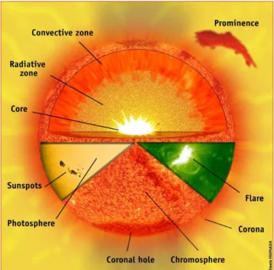
Figure 1.1 – Solar structure, from The Sun Today, C. Alex Young, Ph.D.
1.2.1 Solar Structure
In this topic will be provided some definitions about the solar structure to properly understand various concepts across this dissertation.
1.2.1.1 Core
The core is the most inner part of the Sun, release energy through nuclear fusion when gravity strongly embraces the Sun in a way that hydrogen compresses together to form helium. All the energy that reaches the Earth started in the core of the Sun. The core is highly dense and has a resplendent temperature close to 15 million degrees Celsius (C. Alex Young, 2009).
1.2.1.2 Radiative Zone
The radiative zone is located above the core, this layer of the Sun is where the density slowly decreases when moving away from the core. Nuclear fusion produces light in the core. The light travels out in the shell called the radiative zone. Radiative zone is less dense than the core but it is still enough so that light from the core recoils
4
around taking about 100,000 years to move through this layer and reach convection zone (C. Alex Young, 2009).
1.2.1.3 Convection Zone
This layer above the radiative zone is formed when the density of the radiative zone becomes low enough energy from the core in the form of light is converted into heat. The heat from the edge of the radiative zone rises until it cools enough that it sinks back down. C. Alex Young (2009) described this pattern as heated material rising then cooling into big bubbles called convection cells.
1.2.1.4 Solar Atmosphere
1.2.1.4.1 Photosphere
Photosphere is the origin of the light seen from the Sun. When the material reaches the top of the convection zone, it cools and emits light. This layer is not solid, but it is still called the surface of the Sun and it is also where the solar atmosphere starts. Its temperature is around 5,800 Celsius (C. Alex Young, 2009).
1.2.1.4.2 Chromosphere
This layer of the atmosphere has a thickens of around 2,000 km and a temperature increasing up to about 20,000 degrees Celsius when reaching the top of the chromo-sphere. Unlike the photosphere, the chromosphere light is not white but generally red visible light (C. Alex Young, 2009).
1.2.1.4.3 Corona
The corona starts at around 10,000 km above the solar photosphere, this is the highest layer of the solar atmosphere. The atmosphere of the Sun keeps getting hotter as you move outward from the solar surface. The reason behind this phenomenon is one of the biggest questions of astronomy and solar physics of the 20th and 21st centuries. When you move out to 20,000-25,000 km away from the solar surface, the corona reaches
5
a temperature of around 1-2 million degrees Celsius but has very low density (C. Alex Young, 2009).
1.2.2 Surface of the Sun
1.2.2.1 Sunspots
Sunspots are dark patches in the solar photosphere where strong magnetic field has emerged from below the solar surface, within active regions. The magnetic field plays the most important role in determining the properties of sunspots and by reducing the convective transport of heat from below it is responsible for sunspot darkness and for making sunspots cooler than their surroundings (Solanki, 2003).
Over a solar cycle the number of sunspots varies strongly (Harvey, 1992), from not even one at minimum solar activity to 10 or more of maximum solar activity. Large sunspots occasionally reach diameters of 60000 kilometres while smallest sunspots, more common, reach roughly 3500km in diameter (Bray and Loughhead, 1964). Sun-spots lifetime increases linearly with the maximum size they reach, ranging from a few hours to months. However, their mean lifetime is less than a day (Solanki, 2003).
1.2.2.2 Coronal Bright Points
CBPs are small and bright structures observed in extreme ultraviolet (EUV) and in X-ray frequencies of the solar spectrum. CBPs are present in the solar corona and are associated with bipolar magnetic features. The diameter of around 1-2x10⁴ km and a temperature of around 1.5-2x10⁶ K were estimated (Golub, Krieger and Vaiana, 1976).
Golub et al. (1974) examined the lifetime of 100 bright points, concluding that the majority had a mean lifetime of eight hours and around 1500 CBPs were estimated to be emerging each day.
These bright points can be found at all latitudes of the Sun and in both poles (Fig-ure 1.2). Approximately half of the points are uniformly distributed over the solar corona and the remaining half are confined mostly within 30° of the equator with significant longitudinal variation (Golub, Krieger and Vaiana, 1976).
6
Figure 1.2 – CBP detected in AIA 193 image, from (Chandrashekhar et al., 2013).
1.2.3 Solar Activity
1.2.3.1 Solar Wind
In the last decades, solar wind has been recognised as the main factor controlling the effects of space weather on Earth (Obridko and Vaisberg, 2017). The outer corona is heated up and until it expands away from the Sun as a stream of electrons, protons and other atomic particles. These particles are expelled outside the Sun at speeds of around 200-400 km/s. The solar wind fills the entire solar system, so all the planets sit inside the outer solar atmosphere (C. Alex Young, 2009). Charged particles and magnetic clouds are emitted in all directions as the wind travels outwards, partially reaching our planet.
1.2.3.2 Solar Flares
A solar flare occurs when magnetic energy that has built up in the solar atmos-phere is released, in the form of electromagnetic radiation and very fast atomic particles, resulting in a rapid heating of coronal and chromospheric material (Kahler, 1992). Solar flares occur in regions of concentrated magnetic field such as sunspots in a relatively short amount of time (a few minutes).
7 1.2.3.3 Coronal Mass Ejections (CMEs)
CMEs are the result from closed magnetic field regions in the corona where the solar magnetic field previously was sufficiently strong to constrain the plasma from ex-panding outward (Gosling, 2000). Large fragments of corona material are released out-wards the corona when this becomes disturbed by the release of magnetic energy. While moving out of the Sun, the fragments expand and become as large across as the distance from Earth to Sun (149600000 km) (C. Alex Young, 2009). It has been estimated that CMEs rate is around 5 events/day at activity maximum and less than 1 events/day near activity minimum (Gosling, 2000).
1.3 Importance of Solar Rotation
Nowadays it is believed that the Sun has a magnetic field due to rotation. This field is maintained since the rotation upon convection rises the dynamo action. X-ray data analysis show that chromosphere and coronal emission are known to be well correlated with surface magnetic fields, and as a result the correlation may be interpreted as reflect-ing a close relation between overall level of surface magnetic activity and stellar rotation rate. Such a relation is to be expected based on standard dynamo theory, which predicts increasing field amplification with increasing rotation and differential rotation (Noyes
et al., 1984)
Further investigations revealed that the Sun’s photosphere and chromosphere ro-tation is different. Equatorial zones rotate faster than the polar regions and the latitudi-nal profiles of rotation vary slightly for different features (Figure 1.3). The nature of solar cycle is determined by its differential rotation profile which is influenced by the form and amplitude of the magnetic field.
The large-scale manifestations of solar activity, such as changes in the levels of solar radiation and ejection of solar material, are related to changes in the local magnetic field which may have their origins in variations in the differential rotation. Differential rotation mechanisms and its consequences on the Solar System are still being subject of studies and not fully understood.
8
Figure 1.3 - The mean values of sidereal rotation velocities of CBPs at different lati-tudes, from (Brajsa, R.Wohl, 2002).
1.4 Research Problem
To have an automatic and near real-time solar images processing tool, it is neces-sary to receive these images from the provider as they are captured and available. Find-ing out the rate they are made available, which can change durFind-ing spacecraft manoeu-vres or when a data outage occurs, is also important to avoid downloading duplicated images or excessive requests to the data provider website.
After retrieving the images, these go through a pre-processing algorithm to correct geometry, focusing and exposure. The methods to be applied must be studied to allow an easier identification of the CBPs and get more accurate results.
With the image pre-processed, the next step is to detect and track CBPs. To accom-plish it, it is necessary to choose the more adequate algorithm, since there are several image segmentation strategies (Figure 1.4). It is not always clear which method deliver the finest result and that is why it is so important to update the available algorithms to ensure progression. The CBPs’ travel speed will be the main feature used to calculate solar rotation and all the results must be saved to be visualized later in the webtool.
9
Figure 1.4 - Image segmentation methods.
The CBPs information is saved on a database allowing the webtool to do visual analytics, mainly by displaying plots which can be quickly analysed by the astrophysi-cists. The webtool structure and functionalities, was designed with the help of Dr Ivan Dorotovič from the Slovak Central Observatory in Hurbanovo, Slovakia.
The main challenge is to keep all the process running automatically, from the im-ages retrieval, image processing to the webtool continuous updates. All these steps need to be optimized, in order to have the information displayed in near real-time.
1.5 Dissertation Outline
This dissertation covers 5 chapters that provide detailed knowledge about the work developed. Chapters which are objectively prepared for supporting analysis and introspection is presented next. These chapters are:
Chapter 1: Introduction hosts the first impressions of the work, useful definitions and proposes the implementation approach. The motivations are outlined, and the ar-chitecture is explained.
Chapter 2: State-of-the-Art summarizes the technologies behind the existing algo-rithms for detecting and tracking Coronal Bright Points, highlighting their potential, im-provements and drawbacks. At the end of the chapter there are some general conclu-sions which target the key subjects.
Chapter 3: Implementation exposes the methods and techniques used. Starting with a review about the dataset, explaining the images format and provider service. Sec-ondly, the methods applied in pre-processing to increase the CBP detection efficiency
10
are addressed. Finally, an explanation of each step of the methodology is presented, where the website is also included.
Chapter 4: Results presents the outcomes of applying the tool to a sequence of images, containing different charts, comparisons with other authors’ work and website snapshots.
Chapter 5: Conclusions and Future Work is the last chapter of the dissertation where the results obtained are evaluated. Topics which would most likely improve this subject to achieve better results or complement with additional features the developed software are also proposed.
11
2
S
TATE OF THE
A
RT
This chapter presents the review of algorithms for detecting and tracking Coronal Bright Points and space weather related websites.
Sunspots are commonly used and were also the first tracers used to determine the solar differential rotation profile (Newton and Nunn, 1951). The tracking of sunspots has some advantages, being one of these the long-time coverage due to its extended lifetime. There are also numerous disadvantages associated with tracking this feature: sunspots have complex and evolving structure, their distribution in latitude is highly non-uni-form, and they do not extend to higher solar latitudes. The amount of sunspots during the solar cycle is also unstable, resulting in determination of solar differential rotation profile being really difficult to perform during solar minimum (Sudar et al., 2015).
CBPs propose an improved method to track solar rotation profile, including in minimum solar activity periods, meaning that no active regions are present. CBPs have demonstrated to be great tracers, when comparing with Sunspots. CBPs reach signifi-cantly higher latitudes, they are abundant in all periods of the solar activity cycle while, for instance, sunspots are frequently missing during the minimum of the cycle (Sudar et
al., 2015) and their lifetime ranges from about 2 to 48 hr (Golub, Krieger and Vaiana,
1976). CBPs offer appropriate features for the determination of the solar differential ro-tation also because they are small localized objects and their location is well distributed over the solar corona (Brajša et al., 2001).
12
2.1 Solar data-analysis software
SunPy is a community-developed open-source software library for solar physics. It provides a comprehensive data analysis environment that allows researchers within the field of solar physics to effortlessly carry out their tasks (Mumford et al., 2015).
It was written using the Python programming language and is built upon the sci-entific Python environment. It includes other Python packages such as NumPy, SciPy, Matplotlib and it is a fundamental package within the Python astronomy system.
This package was established on the 28th of March 2011 by a small group of scien-tists and developers at the NASA Goddard Space Flight Center. Since then, SunPy has grown into a larger community.
2.2 Detection and Tracking
The following image processing algorithms present in this topic were selected due to their performance in detecting and tracking CBPs from SDO AIA solar images. The advantages and disadvantages of each algorithm applied to this process are explained ahead.
2.2.1 GPL
Gradient Path Labelling is an innovative segmentation algorithm that was origi-nally developed by (Mora et al., 2011) and applied to segmentation of retinal images. The application of the GPL in the detection of CBPs in solar images can also be successful, since CBPs are small objects with high intensity regions and distinct boundaries between the object and the background (Shahamatnia, Dorotovič, et al., 2016).
The algorithm to detect CBPs is a process with three steps. Starting by pre-pro-cessing the image to decrease noise and get a more accurate segmentation. The second step is the GPL segmentation. Finally, the post-processing consists in a filter to select regions matching a CBP and the computation of their centre of mass location (Figure 2.1).
13
Figure 2.1 – CBPs detecting process, from (Dorotovic, 2017).
The GPL segmentation algorithm performs the pixel labelling procedure by using the image gradient as basis. After that, it groups ascending paths that belong to the same regional intensity maximum. Pixel labelling has the advantage to get a faster segmenta-tion time with a complexity proporsegmenta-tional only to the image resolusegmenta-tion. Its segmentasegmenta-tion result is like the Watershed Transform, with several advantages: having a lower over-segmentation effect, good computation efficiency and customizable over-segmentation effect.
For better results a post-processing algorithm is usually applied after GPL to merge neighbour regions with similar intensities. This results in an image segmented into several intensity regions that are then filtered to match CBPs regions.
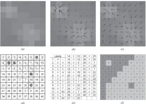
The first stage of the GPL is labelling, this procedure assigns to pixels with similar features a common label, following a top-left to bottom-right direction. It starts by as-signing a new label to each pixel and determining its gradient azimuth using a 3×3 edge detection method, such as Sobel operator, illustrating in Figure 2.2.b the direction to-ward an ascending path.
The next stage is label propagation, this consists in propagation of this label follow-ing the ascendfollow-ing intensity path until findfollow-ing an already marked or outside image boundaries pixel (Figure 2.2.c and 5.d). If this process finishes on a different label, the two labels are tagged as equivalents. The next step of the labelling propagation is to apply equivalence labels, replacing on the image by the smaller one of each group (Fig-ure 2.2.f).
14
Figure 2.2 – GPL labelling method, from (Mora et al., 2011).
When this method is applied to a substantial sequence of images, due to the high-resolution solar images and the GPL segmentation algorithm complexity being propor-tional to the images size, the image is split into smaller regions (a total 4x4 regions) and applying the segmentation in each one separately (Coelho, 2017). Margins were left out and split regions had leaving the margins off, overlapping the split regions and applying the segmentation in each one separately.
The algorithm tends to develop over-segmented results, mainly when there are sub-regions without intensities variations. The output image needs remerging to repre-sent clear CBP structures. The merging process consists on a connectivity graph analysis where adjacent regions are merged if they can be connected by a path that meets the predefined amplitude merging conditions (Mora et al., 2011).
In this method, the tracking of the CBPs if performed by computing the Euclidian distance, with a determined range of pixels, between an object detected in the pre-sent image and the objects in the last three previous images. If no previous object matches the range conditions, then a new identifier it set. Otherwise, the CBP is
at-15
tributed the same identifier as the closet one. The reason to search in three previous im-ages is due to inconsistency in the CBPs activity, causing these to disappear for some minutes and reappear later (Dorotovic, 2017).
2.2.2 PSO/Snake Hybrid Algorithm
This approach was first introduced by (Shahamatnia and Ebadzadeh, 2011) ap-plied on medical imaging. This method has already proved to be also successful in track-ing sunspots (Shahamatnia et al., 2012). In 2013, (Dorotovič et al., 2014) applied this hy-brid method to track Sunspots and CBPs. Later, in 2016, E. Shahamatnia et al. studied the use of this algorithm for calculating solar differential rotation by tracking CBPs.
Particle Swarm Optimization (PSO) is a nature-inspired search algorithm for find-ing the global minimum, but it is particularly useful for solvfind-ing difficult problems, as there are often specific methods for solving easier problems, which are more effective. Due to its flexibility, simplicity of use, implementation and versatility, particle swarm optimization may be applied to many different chemometric fields.
PSO behaves as a population of particles, each like a bird searching for the best place to find food. Each particle in PSO is a candidate solution and these are governed under their cognitive and social behaviours, which make them able to exchange infor-mation and share their experience of explored space, and finally converge towards the optimum of search space, which is the solution to the formulated problem.
First, for detection purpose it is applied Active Contour Model (ACM), also known as Snake model, a technique based on deformable model which was introduced by (Kass, Witkin and Tetzopoulos, 1988) for 2D image segmentation. The idea of this model is to develop a contour under some constraints to match certain image features and has been successfully employed in a variety of problem domains such as object tracking, shape modelling image segmentation and stereo vision. The progress in this model evolves by an energy minimization concept. It comprises of an energy function which should be minimized to find the optimal contour or snake. The function considers the similarity between the contour and the image features, like object boundaries, as well as the similarity of the contour to a prior model contour.
The process starts with setting up the initial contour/curve, defining the snake, therefore, moving towards the object. The snake movement is managed by internal and
16
external forces, within the curve and from the image respectively. These forces are re-sponsible for maintaining the snake shape and steer its way into the object.
Secondly, the tracking approach is implemented by running Particle Swarm Opti-mization (PSO) algorithm. The Swarm is initialized with random solutions. Particles fly through the hyperspace searching for the global optimum. By sharing information within the swarm, particles progressively cluster around the optima. The velocity is con-tinuously adjusted according to the particle’s experience of best position as well as its neighbours’. Particles remember the best position they have discovered according to a fitness evaluation function. This position and its corresponding fitness value are stored as personal best and form the cognitive aspect of particle evolution. Second principle of particle evolution simulates social behaviour and is implemented by tracking the overall best position found within the particle neighbourhood (Shahamatnia et al., 2012).
Figure 2.3 - Block diagram of PSO/Snake algorithm for object detection and tracking, from (Shahamatnia, Mora, et al., 2016).
2.2.3 BP-Finder Algorithm
This automated X-Ray BP detection algorithm was proposed by (McIntosh and Gurman, 2004) as a variant with new features of the former one written in the Iterative Data Language (IDL). The algorithm consists on taking a raw EIT FITS file, which stands for the Extreme Ultraviolet Imaging Telescope on board of the SOHO (Solar and Helio-spheric Observatory) and apply a N×N boxcar smooth function to determine the local background intensity. The smoothed background is subtracted from the original image, and intensity enhancements (BP candidates) are classified by their separation from the background in units of noise level, previously estimated, with some restrictions on size and shape.
17
Martens el al. (2012) improved the original algorithm to include an upper and lower limit on the size of the BPs, weighted by limb angle. Slightly reduce the noise threshold to see if spatially close BPs merge and If so, the underlying ribbon structure is then reassigned. Placed an additional constraint on the ratio of the two major axes of the BP and its perimeter/area ratio to prevent the detection of patches of locally enhanced quiet Sun pixels conglomerations.
When detection is completed, it is performed the total counting of regions and for each one in each bandpass, it is determined the intensity, size, perimeter, major/minor axes and area. The algorithm tracks, in one of the AIA wavelengths, the centre of mass (intensity-weighted) and area with the position compared with projected rotation rate in order to find the lifetime of the BPs. The lifetime is based on their appearance and disappearance or, in longer living ones, from their rotation on and off the disk (Martens
et al., 2012).
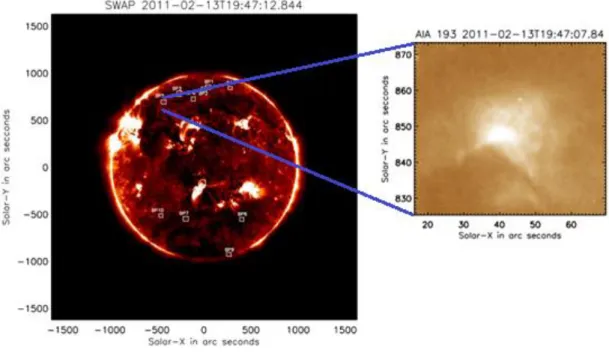
Sudar et al. (2015) successfully employed this algorithm, covering two days (1 and 2 January 2011) with a 10 min time interval between two successive images. This resulted in measurements of 66842 positions of 13646 individual CBPs. The Figure 2.4 shows the distribution of detected CBPs and compare it to the full disk image of the Sun in the 19.3 nm channel obtained on 1 January 2011. White circles show CBPs that were detected on one image by the segmentation algorithm. It is possible to see that there are not many CBPs in active regions, partially because of difficulties in detecting them against such bright and variable.
18
Figure 2.4 - Image of the Sun in the 19.3 nm channel obtained by SDO/AIA on 1st of January 2011. White circles show detected CBPs, from (Sudar et al., 2015).
2.3 Webtools
There are already a few real-time solar tools providing space weather information online, mainly about solar radiation, wind, magnetic field and activity. None of the avail-able tools are focused on solar rotation or CBPs tracking as proposed in this dissertation. In this section the main web tools related to space weather and forecast are reviewed .
2.3.1 Space Weather Prediction Center
The Space Weather Prediction Center (SWPC) (NOAA / NWS Space Weather
Prediction Center) is a laboratory and weather forecasting centre of the National Oceanic
and Atmospheric Administration (NOAA) located in Boulder, Colorado. SWPC contually monitors and forecasts Earth's space environment, providing solar-terrestrial in-formation. NOAA SWPC is the official space weather government agency from the United States that provides alerts, watches and warning for space weather disturbances. The SWPC website not only provides space weather forecasts, but also an array of observed data sets like solar radiation intensities, solar wind, solar corona heating and
19
transient events, magnitude of geomagnetic storms and much more. Many of these data sets are available in near-real-time, and come from a variety of sources, ranging from solar imaging satellites to ground magnetometer stations.
2.3.2 Space Weather Live
Space Weather Live (SpaceWeatherLive.com, 2003) is an initiative of Parsec vzw, a non-profit organization from Belgium which consists of several websites about Astron-omy, Space, Space Weather, aurora and related subjects. The organization promotes these scientific branches onto the world wide web with websites as this one.
In this website is possible to find data about global geomagnetic activity, real-time auroral activity, measurements of low energy electrons and protons carried with the so-lar wind, amount of high energy soso-lar protons at Earth and real-time soso-lar activity, like sunspots and solar flares.
2.3.3 Solar & Heliospheric Observatory
Solar and Heliospheric Observatory (SOHO) (Solar and Heliospheric Observatory, 1995), is a project of international cooperation between ESA and NASA to study the Sun, from its deep core to the outer corona, and the solar wind. Together with ESA’s Cluster mission, SOHO is studying the Sun-Earth interaction from different perspectives.
SOHO provides easily accessible data to the space science community and the gen-eral public as well. This data covers from near real-time images and videos to scientific data like solar radiation, and activity. Most of this data is provided by redirecting to pages located outside the SOHO web site but are obtained by the SOHO instruments.
2.3.4 Solar Influences Data Analysis Center (SIDC)
SIDC (SIDC: The Solar Influences Data analysis Center website, 2006) is the solar phys-ics research department of the Royal Observatory of Belgium. The SIDAC goal is to be the primary reference and source of information on the Sun, solar activity and space weather for all Belgian user communities (general public, schools, industry, authorities and funding agency).
20
This website main features are solar observations from The Uccle Solar Equatorial Table (USET), space weather forecast and real-time alerts. There is also a page denomi-nated Sunspot Index and Long-term Solar Observations (SILSO), dedicated to sunspots number predictions, with a range of 12 months ahead and from 1700 up to the present.
2.4 General Conclusions
Taking in consideration the advantages and disadvantages of the methods re-viewed in this chapter, it is possible to choose those that might me more suitable for this dissertation’s case of study. Most of them have been used in similar applications with positive results. Therefore, some promising conclusion are expected to be reached.
The first step has already been decided, which is the use of CBPs to calculate the solar rotation. The previous investigations concerning this dissertation topic concluded that CBPs have the capacity to provide more accurate tracking characteristics on the en-tire solar corona than sunspots.
The second step is to choose of the right method to detect and track CBPs. Both the methods referred before, GPL and PSO/Snake Hybrid, should produce good results since other authors applied them successfully before. BP-Finder is not an option since it is implemented in IDL and the algorithm in not available as open source. Although, for this dissertation the author decided to use the Gradient Path Labelling for detecting the CBPs and these were tracked searching in the three previous images the closest CBPs, using Euclidean distance.
Finally, investigation on what features the actual available websites are missing that may be scientifically important was considered. This point influenced the idea of creating a new web tool dedicated to the solar rotation and CBPs.
21
3
I
MPLEMENTATION
This chapter describes the implementation procedures, processes, challenges and solutions adopted. Being the fundamental topic of this dissertation, it covers every as-pect in detail for easier understanding and introducing the reader to a further scientific and technical approach to the research problem and the proposed solutions.
3.1 Image Dataset
3.1.1 FITS
Flexible Image Transport System (FITS) is a powerful format for digital image stor-age, transmission and processing. Consisting of multidimensional arrays (images) and 2-dimensional arrays organized into rows and columns of information and easily inter-preted by both humans and computers (Wells, Greisen and Harten, 1981). Because of its great flexibility, the FITS format has been widely used in astronomy.
The FITS file format was standardized in 1981 and has progressed gradually since then. The latest version (4.0) was standardized in 2016. FITS was designed looking to-wards long-term scientific data archival storage. One of the requirements is that devel-opments to the format must be backwards compatible.
When FITS is used for image data, as in this dissertation, it can be as a two dimen-sional array (X, Y) with single values at each point, perhaps some measurement of in-tensity in a particular spectral band or three-dimensional (X, Y, colour) where the third
22
axis illustrates different points on a spectral axis, as measured by wavelength, frequency, or some other appropriate scale. There is no assumption in astronomical analysis or in FITS of a defined colour-space (such as RGB), instead astronomy images are usually ren-dered in colour maps.
The original and still most commonly used type of FITS is representing an image as a header/data block. FITS image headers can contain information about the capture instrument, date and one or more scientific coordinate systems that are overlaid on the image itself. The images header in this work provided additional information such as: Sun radius, the Sun is centred in the image and even the Sun distance from Earth.
Latest versions increased support from 32-bit integers to 64-bit integers in images and tables and allow tables with variable-length arrays. The World Coordinate Systems (WCS) was adopted. This system conventions to map an element in a data array to stand-ard physical coordinates on the sky (Rots et al., 2015).
FITS files contain a single or multiple Header + Data Units (HDUs). The first HDU is called the primary array. The primary array may be empty or contain an N-dimen-sional array of pixels, such as a 1-D spectrum, a 2-D image, or a 3-D data cube. Primary array in FITS support different data types: unsigned 8-bit bytes, 16, 32, and 64-bit signed integers, and 32 and 64-bit single or double precision floating point reals (using the ANSI/IEEE-754 standard, approved by IEEE in 1985). The primary array can be followed by multiple HDUs, called FITS extensions (Hanisch et al., 2001). A FITS file example can be found in Figure 3.1
23
3.1.2 Virtual Solar Observatory
The Virtual Solar Observatory (VSO) is a distributed system that provides users with uniform query interface to access data and images from the major sources of online solar data around the world. It is virtual because it has no physical structure, simply acting as a broker between the user and the data providers (Young et al., 2006). The func-tionality of the VSO is shown in Figure 3.2.
A user can search by time, observables, instruments or spectral range. This searches all data sets for the data in the selected criteria. The primary user interface is a web browser but there are other methods to access data, as the one used in this work, which is part of SunPy package (https://sunpy.org/).
Figure 3.2 - Design of the VSO service. From (Gurman et al., 2005).
3.1.3 Dataset
In this work, the images used were provided by SDO/AIA and obtained automat-ically by querying VSO web service. These images show the sun full-disk as seen in the
24
19.3 nm channel of AIA, with 12 minutes interval between two consecutive images lim-ited by the tool processing speed. They are retrieved with a resolution of 1024 by 1024 pixels (LRi) and AIA level 1.5. Level 1 means that the data have been de-spiked, flat-fielded and the dark current and CCD pedestal removed. Level 1.5 means that the im-ages have been centred and the limb position established (Boerner et al., 2012).
The FITS images in VSO are available in two different resolutions. The first is ap-proximately one hour after capture in 1024x1024 pixels (LRi). The second is approxi-mately 5 days after capture in 4096x4096 pixels (HRi).
GPL segmentation results were compared using: resolution images (LRi); low-resolution images resampled to high-low-resolution (LRRi); and high-low-resolution images (HRi). The tests revealed that LRRi provided more detections (Table 1), by detecting 531 CBPs vs. 443 CBPs with HRi. Although LRRi introduce more false detections, these will be filtered out later. LRi results early revealed to be unpromising (>50% less CBPs com-pared to LRRi and HRi) so was not necessary to continue to study this option.
Therefore, faster results in image pre-processing allied with the significant earlier availability of the images, without compromising the output, are the main advantages for using LRRi.
Table 1 - Comparison between different image resolutions
LRRi HRi
Cadence 3 minutes 10 minutes
Availability on SDO after capture
≈1 hour 5/6 days
AIA calibration level Level 1.5 Level 1
CBPs Detected by GPL on a sample image
25
3.2 Stonyhurst Heliographic Coordinate System
Thompson (2006) pointed some limitations to the use of heliographic coordinates when working with two-dimensional image data, for example, without the r axis, coor-dinates can only be expressed for pixels on the solar disk and features that are elevated above the solar surface will project into coordinates (Θ, Φ) which are different from their true coordinates in a complete (r, Θ, Φ) system.
The Stonyhurst heliographic coordinate system has its origin at the intersection of the solar equator and the central meridian as seen from Earth. This coordinate system remains fixed with respect to Earth, while the Sun rotates. The angles Θ (latitude) and Φ (longitude) are given in degrees, with Θ increasing towards solar North, and Φ increasing towards the solar West as seen in Figure 3.3 (Thompson, 2006). The distance r is either a physical distance in meters, or is relative to the solar photospheric radius R ≈ 6.96 × 10⁸ m.
Figure 3.3 - A diagram of the Sun, also known as a Stonyhurst grid, showing lines of constant Stonyhurst heliographic longitude and latitude on the solar disk, from (Thompson,
26
3.3
Proposed Tool
The tool consists of a Python programme using SunPy (Mumford et al., 2015), As-tropy (The AsAs-tropy Collaboration, 2013) and OpenCV (Bradski and Kaehler, 2000) li-braries in Python (Hughitt et al., 2012) along with GPL for automatic detection of CBPs. The database to store the results was created using MySQL.
The algorithm steps are illustrated in Figure 3.4, using a circular diagram, since the main function is a loop through the sequence of instructions.
First step of the algorithm is to download the lastest SDO/AIA solar images and pre-process them. At this stage the image is ready to be labelled using GPL algorithm, which returns the CBPs detected along with several information about its location, shape, etc. After detecting all CBPs in a single image, each CBP is evaluated in order to successfully be tracked over several images. Finally, the solar rotation is calculated, and the results are presented on the website.
27
3.3.1 FITS Images Acquisition
First step of the software is to download the last SDO/AIA FITS images (1024 by 1024 pixel - LRi) from VSO, using SunPy’s VSOClient method (Figure 3.5).
Figure 3.5 - Python code for querying and downloading images from VSO where tstart and tend are starting time and ending time for the search query. Additional attributes as
In-strument, Wavelength and Cadence are possible.
These images are available 1-2 hours after capture. The algorithm is constantly looking for new images since the cadence rate has oscillations during SDO manoeuvres. This method was chosen since it is compatible with Python language and reliable to query the desired data the from the VSO, searching by date, instrument and resolution. To avoid overloading the server with too many service requests, queries are only submitted after the previous image finished processing and waiting 30 seconds between requests. This time span will not be problematic since the processing time is inferior to the cadence of the SDO/AIA images used.
3.3.2 Pre-processing
Raw AIA Level 1.5 data was corrected at first for the effect of the instrument PSF function using data and method provided by Poduval et al. (2013). Then normalized to values between 0 to 1 using min-max method. Finally, the image is resampled to 4096x4096 pixels using bilinear interpolation.
The comparison between the raw image and the pre-processed image is shown in Figure 3.6 using bronze colour map for easier observation. It is possible to observe that the CBPs are more clear and easier to recognise on the prepared image, mainly due to a more intensive gradient change between the points and the solar corona (background). These prepared images will provide better results when computing GPL.
28
A B
Figure 3.6 – Comparison between raw image (A) and prepared image (B).
3.3.3 CBPs Detection (GPL)
The GPL segmentation method uses the image gradient as the basis for a pixel labelling procedure which groups ascending paths that belong to the same regional max-imum. Together with GPL a post-processing algorithm is applied to merge neighbour regions that have similar amplitudes. The method produces an image segmented in sev-eral intensity regions that are then filtered to match the relevant solar features.
The process starts by creating a mask of the active regions, followed by the GPL segmentation. The generated segmentation regions are then filtered to select the region that matches a CBP and its centre of mass location is determined.
The active regions mask is obtained by applying an Otsu threshold (Coelho, 2017) and performing a morphological open operation (15 erosions and 20 dilations) to clear small manifestations and emphasize the active regions. This mask is then used as fol-lows: if the centroid of the CBP is inside a white pixel, then it should be invalid and, therefore, discarded. An active regions mask example can be seen in Figure 3.8.
Regarding the high-resolution images of the solar disk (16 Megapixels) and the GPL segmentation algorithm complexity being proportional to the images resolution, the images are split into 16 smaller regions and then applied the segmentation in each one separately. This approach enables faster processing when applied to a large dataset.
29
Upon the image splitting the image borders were left off and split regions were over-lapped (both horizontal and vertical) to ensure no CBP is missed. To avoid duplicate detections in the overlapped regions a postprocessing is applied to discard the CBPs that are on the outermost half of the overlap region.
GPL was configured to select only small area objects (less than 5000 pixels), alt-hough it still produces an over-segmented image. The GPL merge postprocessing is then reapplied, grouping neighbour objects and rejecting oversized objects. The result of remerging and corrected over-segmented CBPs can be seen in Figure 3.7.
Finally, detected CBPs are filtered to discard those near the solar limb due to being more imprecise, and those located inside the active regions mask (see Figure 3.7). More-over, objects centroid and maximum intensity coordinates (in pixels) are recorded in a database to later study the solar rotational profile.
An example of CBPs identifications, detected in one SDO/AIA image sample, is shown in Figure 3.9 where CBPs’ brightest points are the centre of the blue circumfer-ences.
Figure 3.7 – GPL merging illustration. Before merge and active regions mask filter on the left image. After remerging and active regions mask filter on the right image.
30
Figure 3.8 - Sun disk binarization. This mask is used to discard CBPs inside active re-gions (white pixels).
Figure 3.9 - CBPs detection in a single SDO/AIA image. Active regions were clearly avoided. There is no relation with the previous figure since the capture dates are different
31
3.3.4 CBPs Tracking
The CBPs brightest point, provided by GPL, is used to define its location. Alt-hough, centroid would be more precise, more imprecision than maximum intensity lo-cation due to CBP shape modifilo-cations along the tracking period was shown. The CBP location coordinates will be stored in a database, along with other information.
Tracking of active CBPs is performed over the data stored on the databas, as pre-sented in Figure 3.11. It starts by converting their location in pixels to heliographic Ston-yhurst system for more accurate results. This conversion is performed using the code written in Figure 3.10, where a SunPy method converts the location present in the FITS header of an image to the respective heliographic Stonyhurst system.
Figure 3.10 - Python code to convert coordinates in pixel to heliographic Stonyhurst co-ordinates system. SunPy package is used to perform the pixel_to_world(x, y, origin) function.
The next step is to calculate of the distance (in degrees) between each detected CBP (dCBP) and every active CBP (aCBP), taking in consideration the time span between im-age captures. A aCBP and dCBP are considered to be the same for a maximum distance between the two of 0.4°, if the aCBP was last detected until 30 minutes ago, or 0.8° if detected between 30 and 60 minutes ago. Those maximum distance values were ob-tained by checking on Sudar et al. (2015) the maximum travel of a CBP during a certain period, which was ≈19°/day. This was the tracking principle for knowing if a CBP is an already existing or new one. The restrictions applied in this step are based on Sudar’s (2015) work, limiting data to 85% of the solar disc radius or ±58° from the centre of the sun.
In case of a new CBP, its location, both in pixels and heliographic coordinates, and detection date are saved. Otherwise, it is updated the last location, last detection date, lifetime, distance travelled (in degrees) and number of detections in different images.
32
After processing each image, the tool loops through every active CBP to check if it should be set as non-active. It is considered a CBP to be non-active after 60 minutes with-out being detected, since CBPs might not be visible for a few minutes despite being still active. Non-active CBPs remain in the database for website archive purposes.
Figure 3.11 - CBPs detection algorithm flow chart. Distance response takes in consider-ation the time span between captures as explained previously.
33
3.3.5 Solar Rotation Calculations
Finally, the solar rotation speed is computed using the travelled distance and life-time of each detected CBP. To acquire more accurate velocities, possible outliers are re-moved using similar criteria used by Sudar et al. (2015), mainly removing the CBPs with less than 10 identifications (120 minutes), restricting the sidereal rotation speed to 8° < 𝑣𝑒𝑙𝑟𝑜𝑡 < 19° day-1. An addition filter was included to remove the CBPs with reduced ra-tio of detecra-tions, remaining only those that were present in at least 75% of the images during its lifetime. Although these CBPs can be used, their uncertainty may increase the error on the solar rotational speed assessment.
The CBP motion was approximated with a linear fit to calculate the synodic veloc-ity with equation (1),
𝜔
𝑠𝑦𝑛=
𝑁 ∑
𝑁𝑖=1𝑙
𝑖𝑡
𝑖− ∑
𝑁𝑖=1𝑙
𝑖∑
𝑁𝑖=1𝑡
𝑖𝑁 ∑
𝑁𝑖=1𝑡
𝑖2− (∑
𝑁𝑖=1𝑡
𝑖)
2(1)
where N is number of identifications, 𝑙𝑖 is the central meridian distance (CMD), 𝑡𝑖 is the lifetime of the CBP and 𝑏𝑖 is the latitude of each measurement for a single CBP. To obtain the true rotation of CBPs on the Sun, it is required to convert synodic (apparent) velocities to sidereal (true) using Eq. (7) from Skokic et al. (2014), which pro-vides more accuracy, since it takes in consideration the current orbital angular velocity of Earth, instead of a mean value. If this effect is not considered, it can introduce a sys-tematic error in solar rotation studies. The solar ephemeris parameters required for this conversion are returned from SunPy when a date is supplied. The Python code to make this conversion is presented in Figure 3.12. The values obtained from SunPy were com-pared with ALMA Solar Ephemeris Generator (I. Skokić, 2015), revealing an accurate approximation.
34
Figure 3.12 – Python code with SunPy package to acquire solar ephemeris parameters for a specific date to calculate the sidereal rotation from the synodic rotation.
3.4 Website
The tool and updated results are available at the website of the Space-Planetary Interactions monitoring and forecasting Laboratory of the Geophysics and Astronomy Observatory, Coimbra, Portugal (SPINLab) (Figure 3.13). This web portal that available the most recent solar activity data that allow to follow the Space Weather conditions (http://www.mat.uc.pt/~obsv/SPINLab/SPINLab_solSDO.php). A preview of the CBPs related webpage can be seen in Figure 3.14.
The web interface of our tool (CBPs Tracker) was developed using HTML with CSS and JavaScript for the front-end and using PHP for the back-end. It is supported by a MySQL database. The generated solar data is displayed in charts from the Highcharts library (https://www.highcharts.com/).
The up-to-date solar rotation profile and the active tracked CBPs information is shown. The information is presented with charts and tables. Search and data retrieval from older observations are also available in the archive by defining a starting and end-ing datetime.
Website data regarding CBPs tracking and solar rotation can be exported to CVS or XLS files for external analysis. Charts exporting is also possible as different image formats or PDF.
35
Figure 3.13 - SPINLab website homepage.
Figure 3.14 – SpinLAB website snapshot from CBPs Tracker page. This page can be ac-cessed from Solar data → Uninova menu on the left side.
37
4
R
ESULTS
4.1 CBPs Detection
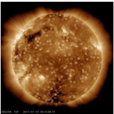
The tool was tested for 4 days, from the 12th to the 15th of August 2018, evaluating a total of 480 images, from which 173666 CBPs individual identifications were obtained. In Figure 4.1 some samples of the image sequence, one per day are illustrated. So, it is possible to observe the solar activity during the testing period.
38
Figure 4.1 – SDO/AIA samples from the testing period, one image per day. Top left from the 12th, top right from the 13th, bottom left from the 14th and bottom right from the 15th
of August.
After filtering out the outliers, using the procedure previously explained, 2029 tracked CBPs. These CBPs are well distributed along all latitudes over the solar corona as illustrated in Figure 4.2. Clearly some areas on the north pole have less detections, due to the lower solar activity (coronal holes).