Thesis
Master of Computer Engineering
Indoor Positioning System for Mobile Devices using
Radio Frequency and Perfect Sequences
(Sistema de localização automática de dispositivos móveis com recurso à
sequências perfeitas de rádio frequência)
Josip Bagarić
Thesis
Master of Computer Engineering
Indoor Positioning System for Mobile Devices using
Radio Frequency and Perfect Sequences
(Sistema de localização automática de dispositivos móveis com recurso à
sequências perfeitas de rádio frequência)
Josip Bagarić
Master's thesis carried out under the guidance of Dr. João da Silva Pereira, professor of the School of Technology and Management of the Polytechnic Institute of Leiria.
v
Dedication
This thesis was made possible by the continuous support of my friends and family. I would like to dedicate this thesis to my parents Milan and Jadranka Bagarić, who support my every action.
vii
Acknowledgements
First and foremost, I would like to express my gratitude to my mentor Prof. João da Silva Pereira for his continuous support, guidance, knowledge and patience with me while working on this thesis. Without his help, the completion of this thesis would not be possible.
Secondly, I would like to thank Instituto Politécnico de Leiria, Escola Superior de Tecnologia e Gestão for providing me with the space and resources to work on and finish the thesis.
ix
Summary
Keywords: indoor, positioning, system, radio, frequency, perfect, sequences, opdg, zigbee, golay, chu, modulation, raspberry pi, accf, standing, wave, cancellation, transmitters.
xi
Abstract
Recent advancements in the area of nanotechnology have brought us into a new age of pervasive computing devices. These computing devices grow ever smaller and are being used in ways which were unimaginable before. Recent interest in developing a precise indoor positioning system, as opposed to existing outdoor systems, has given way to much research heading into the area. The use of these small computing devices offers many conveniences for usage in indoor positioning systems. This thesis will deal with using small computing devices Raspberry Pi’s to enable and improve position estimation of mobile devices within closed spaces. The newly patented Orthogonal Perfect DFT Golay coding sequences will be used inside this scenario, and their positioning properties will be tested. After that, testing and comparisons with other coding sequences will be done.
xiii
List of Figures
Figure 1: Transition to distributed systems ... 25
Figure 2: Mobile computing system... 26
Figure 3: Smart home ... 27
Figure 4: Wifarer [27] ... 36
Figure 5: IndoorAtlas [29] ... 37
Figure 6: Pozyx system elements ... 38
Figure 7: ByteLight business model ... 39
Figure 8: Carrefour smartphone app - uses Phillips' IPS ... 40
Figure 9: Autocorrelation vs. Cross-correlation [39] ... 45
Figure 10: Normalized absolute periodic autocorrelation - ZigBee pseudorandom noise (PN) codes, with a resolution of 16 bits. ... 51
Figure 11: Normalized absolute periodic autocorrelation – OPDG codes, with a resolution of 16 bits. ... 52
Figure 12: Normalized absolute periodic autocorrelation - OPDG codes with the code length of 128, with a resolution of 16 bits ... 52
Figure 13: Standing wave cancellation ... 54
Figure 14: Standing Wave Cancellation - Mechanism ... 55
Figure 15: Indoor Positioning System - Network Topology ... 56
Figure 16: The Raspberry Pi ... 57
Figure 17: Si4703 FM Tuner ... 58
Figure 18: FM receiver module ... 59
Figure 19: Si4703 to Raspberry Pi connection ... 60
Figure 20: FM Transmitter ... 61
Figure 21: IPS - simplified scenario ... 62
xiv
Figure 23: Receiver software flowchart ... 64
Figure 24: TCP Communication - Transmitter to Receiver ... 65
Figure 25: ACCF Ratio calculation ... 65
Figure 26: FM Transmitter - Antenna connection ... 68
Figure 27: Linear scenario ... 73
Figure 28: Test scenario 1 - Results ... 74
Figure 29: Test scenario 2 - Results ... 75
Figure 30: Test scenario 3 - Results ... 76
Figure 31: Test scenario 4 ... 77
Figure 32: Test scenario 4 - Results ... 79
Figure 33: Test scenario 5 ... 79
Figure 34: ACCF measurements - ZigBee vs. OPDG ... 81
Figure 35: Test results – Golay, Chu, ZigBee and OPDG ... 82
Figure 36: Triangulation process ... 83
xv
List of Tables
Table 1: Test Scenario 1 - Parameters ... 74 Table 2: Test scenario 2 - Parameters ... 75 Table 3: Test scenario 3 - Parameters ... 76 Table 4: Average indoor location estimation error between two transmitters - Golay, Chu, ZigBee and OPDG ... 83 Table 5: Influence radii of transmitters ... 84 Table 6: Average indoor location estimation error in a scenario with four transmitters – Golay, Chu, ZigBee and OPDG ... 85
xvii
List of Equations
Equation 1: Discrete Fourier Transform (DFT) ... 45
Equation 2: Inverse Discrete Fourier Transform (IDFT) ... 45
Equation 3: Periodic cross-correlation between two different sequences ... 45
Equation 4: Periodic cross-correlation between two different sequences (alternate) ... 46
Equation 5: Generic algorithm for Golay sequence generation ... 47
Equation 6: Polyphase perfect sequences ... 48
Equation 7: IDFT to DFT ... 48
Equation 8: Recursive algorithm ... 48
Equation 9: Recursive decoding method ... 49
Equation 10: Vector A ... 49
Equation 11: Decoding process - First method ... 49
Equation 12: Decoding process - Second method ... 49
xix
List of Acronyms
ACCF Autocorrelation Crest Factor
AN Antinode
AOA Angle-of-arrival
BLE Bluetooth Low Energy
CDMA Code-Division Multiple Access
CEO Chief Executive Officer
COTS Commercial off-the-shelf
DFT Discrete Fourier Transform
DOP Dilution Of Precision
DPDT Double Pole Double Throw
DS-CDMA Direct-Sequence Code-Division Multiple Access
DVD Digital Versatile Disc
FM Frequency Modulation
GPIO General-Purpose Input/Output
GPS Global Positioning System
HF High Frequency
IDFT Inverse Discrete Fourier Transform
IM/DD Intensity Modulation and Direct Detection
IPS Indoor Positioning System
LED Light-emitting Diode
LOS Line-of-sight
MPI Multipath Interference
N Node
xx
NLOS Non-line-of-sight
OPDG Orthogonal Perfect DFT Golay
PC Personal Computer
PN Pseudorandom Noise
RFID Radio Frequency Identification
RSS Received Signal Strength
SCP Secure Copy Protocol
SFTP Secure File Transfer Protocol
TCP Transmission Control Protocol
TDM Time-Division Multiplexing
TDM-CDMA Time-Division Multiplexing and Code-Division Multiple Access TDOA Time-difference-of-arrival
TOA Time-of-arrival
USB Universal Serial Bus
UWB Ultra-wideband
VLC Visible Light Communication
WAV Waveform Audio File Format
xxi
Index
Dedication ... v Acknowledgements ... vii Summary ... ix Abstract ... xiList of Figures ... xiii
List of Tables ... xv
List of Equations ... xvii
List of Acronyms ... xix
Index ... xxi
Introduction ... 25
Bibliography review ... 31
1.1. State of the art ... 31
Research ... 33
Commercial ... 36
Methodology ... 41
1.2. Received Signal Strength and Triangulation ... 43
1.3. Autocorrelation and Cross-correlation ... 44
1.4. Orthogonal Perfect DFT Golay coding sequences ... 47
xxii 1.6. Standing Wave Cancellation ... 53 1.7. Indoor Positioning System... 56 Raspberry Pi ... 57 FM Receiver Module ... 58 Control Software ... 61 Setting up ... 67 1.8. Transmitters ... 68 Hardware ... 68 Software ... 68 1.9. Receiver ... 70 Hardware ... 70 Software ... 70 Tests ... 73 1.10. Linear scenario tests ... 73 Test scenario 1 ... 74 Test scenario 2 ... 75 Test scenario 3 ... 76 1.11. Two-dimensional scenario tests ... 77 Test scenario 4 - TDM ... 77 Test scenario 5 – Simultaneous emitting ... 79 Results ... 81 Conclusion ... 87 Future work ... 89 Bibliography ... 91
xxiii Appendices and attachments ... 97
Appendix I – Scientific Paper ... 98 Appendix 2 – Scientific Paper ... 119 Appendix 3 – Patent ... 129
25
Introduction
Looking at the world in which we live in, there is no denial that technology makes a big part of our everyday lives. Wherever we go, whatever we do, technology follows us and helps us on the way. Computers (big and small) make a big part of this technology. Computing has been constantly evolving since the arrival of the first personal computers (PC’s) [1]. To this day, computing has gone through a number of revolutions to get to the point in which it is now.
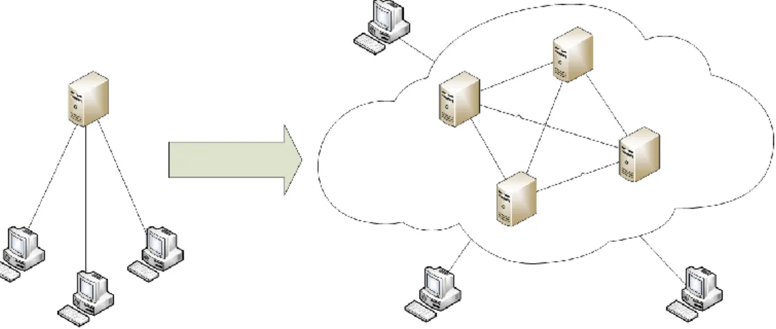
The first revolution in computing happened with the emergence of distributed systems [2]. Distributed systems imply a collection of (static) computers, which are interconnected and work to achieve a certain purpose, as can be seen in Figure 1. These systems transformed the way we work. By implementing distributed systems of computers into the workplace, classrooms and other places, many of the tasks done before started being automated, thus making them easier to do by introducing fault-tolerance. Distributed systems also provided us with remote access to information, remote communication between computers, distributed security and high availability.
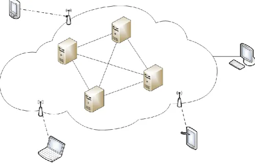
26 The second revolution in computing arrived in the form of mobile computing [3]. Mobile computing was built on the current distributed systems, and brought many improvements that transformed the computing space. It allowed for networking and information access on the go, which is the main feature in today’s workspaces and homes (Figure 2). It also allowed for location sensitivity, application adaptiveness and energy awareness in computing systems. These improvements have transformed (and are still transforming) the way we work, live, play and learn.
Figure 2: Mobile computing system
While the mobile computing trend has taken a major swing in our lives, there is another trend in computing slowly approaching. A new revolution in computing is called pervasive computing, sometimes called ubiquitous computing [4]. This trend in computing takes computing to a whole other level.
Pervasive computing has different goals in mind when compared to the distributed systems and mobile computing. The main goal of pervasive computing is to remove technology from the eyes of the user, while still enhancing the user’s life. The main distinction between pervasive systems and other systems is the fact that it is context-aware.
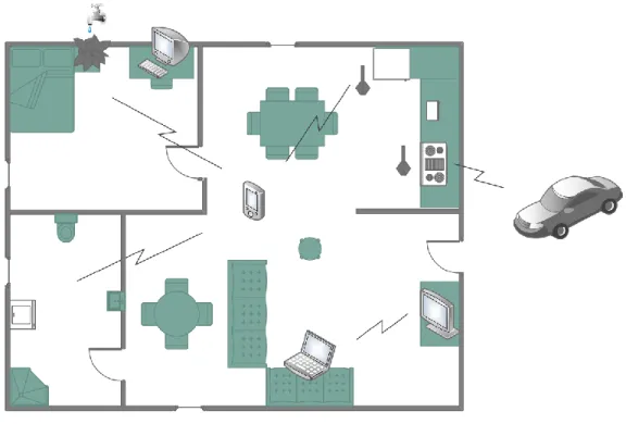
27 An example of pervasive computing are smart spaces (smart houses, smart streets). These spaces help the user with his everyday chores at home and elsewhere, while not providing him the details of how they do it. They take input from our environment, and adjust certain parameters of our environment dynamically and autonomously. One example of such action would be adjusting the air conditioning temperature inside closed spaces depending on the temperature outside the space, so that is never exceeds the difference of 7 degrees Celsius and never drops under the standard room temperature. This makes the user unaware of how the actual system works. It just works, and the user always expects the optimal temperature without his intervention.
Figure 3: Smart home
In Figure 3 you can see an example of how a smart home would function. A smart home serves as a great example of a pervasive system. After being woken up by an alarm clock (depending on your online calendar) your breakfast starts getting ready and your coffee is being prepared as you get out of bed. After getting out of bed you sit at the table and eat your breakfast and drink your coffee. The water in your shower starts to warm up, and your washing machine sends you a notification to your phone that the laundry you left to wash during the night is finished. After taking a shower, you get dressed and start walking towards the car. As you exit the house, your refrigerator
28 sends you a message, telling you that your milk has expired and that you should buy more when returning home. As you approach the car, the car unlocks itself. Sensing that the temperature outside is low, the car starts the engine a few minutes earlier to warm it up, to avoid the possibility of you being late for work. You sit in your car and the car autonomously drives you to work, taking the most optimal road with the least traffic.
Besides the example above, pervasive computing encompasses a huge number of different computing devices, serving many purposes, and has a huge potential in improving life standard, automating mundane tasks, improving business analytics, improving traffic safety, and many other areas. That is one of the reasons why lots of research and development has been going on in this area in recent years.
Here, we will focus on a specific part of pervasive systems, called the Indoor Positioning System (IPS).
Indoor positioning systems are able to estimate the location of entities inside closed spaces. Many types of positioning systems depend, to varying degrees, on line-of-sight (LOS) between transmitters and receivers, as does the conventional well-known Global Positioning System (GPS). These systems allow for accurate outdoor location estimation approximately around 3 meters (best case scenario), dependent on the GPS system, propagation errors, signal multipath, receiver clock errors, GPS satellite orbit errors, number of satellites in LOS, satellite position geometry and the variation in atmospheric conditions. These are computed in terms of GPS dilution of precision (DOP).
Indoor, underground and heavy woods environments (among others) are not suitable for GPS as only minimal and/or partial LOS can be achieved causing lack of coverage and insufficient accuracy in estimation. Additionally, for a positioning system to be usable indoors, the error of estimation has to be lowered from meters to centimeters, as the estimation error in meters would often fail to estimate the correct location of an entity or object.
29 This thesis will deal with researching into the topic of indoor positioning systems [5]. The methodology of implementing an IPS will be explained. All of the related technologies and methods will be explained in detail, and the purpose of these will be shown. After that, a model of the IPS will be created and shown. Testing scenarios will be set up, tests performed and results displayed.
This work was based on my research published in the following publications:
M. Ferreira, J. Bagarić, Jose M. Lanza-Gutierrez, S. Priem-Mendes, J. S. Pereira, Juan A. Gomez-Pulido, On the Use of Perfect Sequences and Genetic Algorithms
for Estimating the Indoor Location of Wireless Sensors, International Journal of
Distributed Sensor Networks, April 22, 2015 [6]
J. Bagarić, M. Ferreira, J. S. Pereira, S. Priem-Mendes, Estimating Indoor Location
Using Wireless Communication Between Sensors, ConfTele 2015, Conference on
Telecommunications - Aveiro, Portugal, September 18, 2015 [7]
J. Bagarić, J. S. Pereira, S. Priem-Mendes, Standing Wave Cancellation – Wireless
Transmitter, Receiver, System and Respective Method, Submitted patent,
31
Bibliography review
1.1. State of the art
With the current pace of technological advancements, the need of an NLOS positioning system grows ever larger. The omnipresence of small and powerful computer and processing units has given way to practical uses of NLOS positioning systems, mainly focusing on indoor scenarios. Taking into consideration the well-known example of the GPS [9], we can display the amount of factors that are being taken into consideration in order to estimate the location of the receiver. Some of these factors include propagation errors, which occur when the signal propagates through the troposphere, and signal multipath, which occurs when the signal is reflected from different entities, resulting in a delay due to the extra time it takes to get to the receiver. Other factors include mismatches in clock between satellites and the receivers, deviations in the satellite orbit, number of satellites visible, etc. While the errors in indoor positioning systems are also influenced by some of these factors, there are also a number of additional factors that have to be taken into account when building an IPS.
Indoor position of a receiver can be calculated in a multitude of ways. A popular method of calculating the indoor position is to use some of the wireless technologies available today. Many of the systems try to use existing (or new) Wi-Fi access points to create a Wi-Fi Positioning System (WPS) by measuring the received signal strength (RSS) for each of the available access points, and then calculating the position accordingly. The problem with WPS is its lack of precision due to the possible signal fluctuations that may occur, increasing errors and inaccuracies.
Another way to calculate the position would be to use compass chips to determine magnetic positioning. By sensing and recording the local magnetic variations caused by the iron in the buildings, a compass (e.g. inside a regular smartphone) would be able to map the indoor location
32 with the accuracy of 1-2 meters. While the error margin of this method is considered to be low, it still does not yield results that are accurate enough to be useful in purposes where centimeters make a difference.
Bluetooth [10] is another example using wireless communication, however it is known to be an indoor proximity solution, not an indoor positioning solution. It is mostly used for geo-fencing and micro-fencing.
Radio frequency identification (RFID) [11] can also be used for indoor positioning but, despite its cost–effectiveness, it does not support any metrics. Visible light communication (VLC) also grants some positioning properties, where indoor lighting can be used as a transmitter of information, and a smartphone camera can be used to detect changes in light to determine its location based on the source that emits it. This method can yield accuracies up to decimeters, but suffers of sporadic detection points. Tango Google Project is one of such VCL examples.
Ultra-wideband (UWB) [12] can also be a viable solution for positioning purposes, as it provides location accuracy up to 10 cm. UWB uses brief bursts of radio energy, akin to some radars, and then measures the time it takes for the signal to reach the other receivers. This avoids the multipath problems due to the brevity of the radio wave. While this gives accurate results, the problem is that UWB waves get blocked very easily, around 40 percent of the time.
Using ultrasound for indoor positioning has also received quite a bit of attention, due to the high accuracy of its slow-moving waves. Ultrasound can be used to track and identify the location of objects using inexpensive tags embedded into devices which provide ultrasound sensors with their location. The shortcoming of this technology is its short range, which makes it impractical in many situations, despite its high accuracy and robustness when compared to radio technologies, where the waves can pass through the walls more easily than ultrasounds.
33
Research
In this section we investigate the different approaches that are currently being researched. 1.1.1.1. Ultrasonic positioning systems
A number of ongoing researches have been dealing with ultrasound as a media for indoor positioning.
Indoor Positioning for Smartphones Using Asynchronous Ultrasound Trilateration [13] proposes
a system that uses regular commercial off-the-shelf (COTS) hardware such as smartphones to determine the indoor position of the user. In their research, they have proven that a very short 21.5 kHz ultrasound “beep” emitted from a smartphone and received by four receivers in the corners of the room can lead to errors lower than 1 meter (averaging around 10 cm in their research). The receivers use a TDOA (Time-Difference-of-Arrival) or the asynchronous approach to determine the distance of each receiver and the smartphone. While this approach, so called Ultrasound trilateration, seems promising, the directional nature of ultrasound, it’s susceptibility to certain high frequency background noises, and the need for line-of-sight between speaker and receiver were identified as the biggest obstacles to positioning accuracy.
1.1.1.2. Wi-Fi
In order to mitigate many of the problems in Wi-Fi positioning, WLocator: An Indoor Positioning
System [14] introduces a few improvements to the IPS system. Dealing with fluctuation, fingerprint
management and location-aware application development are some of the principles and algorithms introduced, along with performance changes and lightweight software. This system is expanded in WHLocator: Hybrid Indoor Positioning System [15] by combining the WiFi positioning with altimeter and image sensors, and results in higher accuracies in 3D scenarios. By implementing the transmission of multiple predefined messages WiFi-based indoor positioning [16] maintains the high-accuracy of other Wi-Fi based IPS, while at the same time reducing the need for a large number of antennas and relaxing the need for wide signal bandwidth. Their simulation results show that this approach can achieve 1 m accuracy, boasting no hardware changes in commercial WiFi products.
34 Researchers at MIT’s Computer Science and Artificial Intelligence lab have managed to achieve decimeter-level IPS accuracy with their novel Chronos [17] technology. This technology works with a single access point and off-the-shelf Wi-Fi cards, and uses time-of-arrival calculation between a receiver and transmitter to localize them. It does so by making the receiver and transmitter to hop between all 35 frequency bands in the 2.4 GHz to 5.8 GHz range. This changes the rate at which signals accumulate phase for each of the frequencies, which is then used by Chronos to calculate the time-of-arrival of signals and estimate the distance. Some tests have managed to localize devices to within 65 centimeters.
1.1.1.3. Visible Light Communication
An Indoor Visible Light Communication Positioning System Using a RF Carrier Allocation Technique [18] proposes an indoor positioning system that adopts Visible Light Communication
(VLC) that is based on the intensity modulation and direct detection (IM/DD) in a line-of-sight environment. They investigated this principle by simulations and experiments and found that, although it was inaccurate when estimating distance based on the effects of radiation directivity and the incidence angle, the positioning error would be reduced when the adjustment process by normalizing method is used. Their results show that the average error of estimated positions can be reduced to 2.4 cm using, which is compared with 141.1 cm without the adjustment process.
On the other hand, Indoor Positioning System Using Visible Light and Accelerometer [19] proposes a different approach to VLC, by complementing the IPS system with the results of the smartphone’s accelerometer. The system uses the accelerometer to detect the orientation of the device, and uses the light sensor to detect the received light intensity. Their low-complexity algorithm requires no knowledge of the LED transmitters’ physical parameters, and their tests show it is possible to achieve an average position error of less than 0.25 m.
1.1.1.4. Radio Frequency Identification
A Standalone RFID Indoor Positioning System Using Passive Tags [20] suggests an indoor
positioning system based on RFID. This kind of IPS system proposes that small RFID tags are set up around the space. As the user moves through the space, the receiver object would pick up the
35 signals from these tags, and determine its location based on the signal provided by these RFID tags.
Development of an Indoor Navigation System Using NFC Technology [21] proposes a similar
solution, but uses Near-Field Communication (NFC) [22], a branch of High Frequency (HF) RFID. 1.1.1.5. Geomagnetism
Indoor positioning system using geomagnetic anomalies for smartphones [23] proposes a novel
technique that makes use of the perturbations of the geomagnetic field caused by structural steel elements in a building. The advantage of this system is that it does not require any sort of physical infrastructure, which makes it a very cost-effective solution. After a building has been mapped, and its magnetic footprint recorded, a target’s position could be estimated by comparing the sensor measurement of a device (e.g. smartphone) to the measurements on the magnetic footprint of the building. Their results show that the accuracy of such a system is within 3 meters.
1.1.1.6. Hybrid
Instead of building an IPS system using a single technology, some IPS systems combine more technologies that complement each other and improve the accuracy.
Hybrid Indoor Positioning with Wi-Fi and Bluetooth: Architecture and Performance [24] does just
that. In their scenario, a Wi-Fi based position estimation method is used, and is enhanced by using Bluetooth hotspot devices. The Bluetooth devices help the Wi-Fi IPS by partitioning the indoor space using the divide-and-conquer method.
Redpin - Adaptive, Zero-Configuration Indoor Localization through User Collaboration [25]
describes an open source indoor positioning system that was developed with an aim to allow for at least room-level accuracy. Additionally, it introduces an alternative to time-consuming training phases by incorporating a system that enables the users to train the IPS system as they use it. Redpin works with standard GSM, Wi-Fi or other wireless technologies that mobile phones implement.
36
Commercial
On the commercial side, there a few IPS systems available, some of which will be described in this section.
1.1.2.1. Wifarer
One example of a commercial IP system is Wifarer [26]. In order to enable indoor positioning inside a closed location, Wifarer needs to map the indoor space. It does so by scanning the fingerprint of Wi-Fi or Bluetooth LE (BLE) networks. It uses the signal strength of nearby networks, and maps it to a certain point inside the indoor space. Once the whole indoor space has been mapped, it enables indoor positioning and navigation.
Figure 4: Wifarer [27]
The error of the Wifarer system greatly depends on the amount of Wi-Fi and Bluetooth LE networks are present inside the indoor space, but for areas with dense Wi-Fi networks such as airports and bus stations, Wifarer’s CEO boasts an error as low as half a meter. The advantages
37 using Wifarer are that it can be installed on any smartphone that has a magnetometer/compass, and can be used straight away.
1.1.2.2. IndoorAtlas
Another contender in the commercial space is IndoorAtlas [28]. IndoorAtlas platform takes a more innovative approach to indoor positioning by using the magnetic footprint of buildings to map the indoor space. Same as with Wifarer, the advantage of IndoorAtlas is that it can be installed on any smartphone that has a magnetometer/compass, and can be used straight away.
Figure 5: IndoorAtlas [29]
The user installs the IndoorAtlas app, uploads a map of the indoor space to the application, and starts mapping the space. For the indoor positioning to take place, the user first has to map the space by walking around the building and capturing the magnetic footprint at a large amount of points inside the building.
After the mapping is complete, the indoor positioning can take place. When off-the-shelf handsets are used, IndoorAtlas boasts an accuracy typically less than 3 meters.
38 1.1.2.3. Pozyx
For indoor positioning developers, another hope arose when in 2015, a new campaign started on Kickstarter. Pozyx [30] was founded by a group of developers in Brussels, Belgium, and their aim was to use the existing Ultra-wideband technology to develop an accurate IPS system.
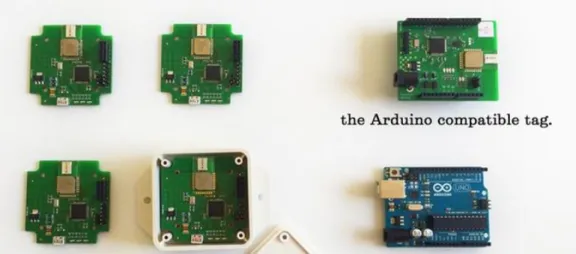
Figure 6: Pozyx system elements
The Pozyx system consists of four anchors (UWB transmitters) and a tag (UWB receiver). After the anchors are set up around the indoor scenario, the tag can be used to compute the indoor location of the device. Pozyx comes with an Arduino library and can be programmed to suit different purposes and can be embedded into different devices.
1.1.2.4. ByteLight
Developers at AcuityBrands [31] took on the approach of using Visible Light Communication to implement their indoor positioning system. They use the indoor positioning to allow the retailers to pinpoint certain objects to their clients, thereby custom-tailoring their shopping experience.
39
Figure 7: ByteLight business model
ByteLight uses the flickering of the light-emitting diodes (LEDs) to determine the location of the user, and uses that location to present them with special offers.
1.1.2.5. Phillips’ LED-based IPS
In 2015, in a Carrefour supermarket in Lille, France, Philips has implemented their IPS system, and this enabling for one of the first IPS-enabled supermarkets.
Phillips bases their IPS on the existing VLC technologies. Every LED lamp that is a part of the IPS system emits a specific code, which is then registered by the user’s smartphone (with the corresponding smartphone app) and then used to calculate the indoor position. Phillips boasts a sub-meter accuracy with their IPS.
40
Figure 8: Carrefour smartphone app - uses Phillips' IPS
1.1.2.6. Nextome
Nextome [32] was formed by three young graduate students from Puglia, Italy. The decided to use the newly created Apple’s standard called iBeacon [33] to implement their IPS, combined with Bluetooth Low Energy (BLE). iBeacons would be used as BLE transmitters and set up around the indoor scenario. After that, a BLE 4.0 enabled smartphone (Android or iOS) would be used to detect its indoor position.
Nextome use a new localization method, called MLV3. This method limits the “path fading” effect by removing signal interferences bouncing off walls, floors and other indoor objects. Additionally, they use Intelliwalk [34] technology to detect in which direction the user is moving, which requires the phone to have a gyroscope, a magnetometer, a compass and other (these days) standard phone sensors. Lastly, they use particle filtering (Sequential Montecarlo Filtering [35]) to on the map information, which removes the odds of user being positioned in an unreachable zone and saves the energy and battery of the smartphone.
41
Methodology
This section describes the related technologies used inside the IPS system, as well as the methods used to achieve results.
There are a number of factors that need to be taken into account when building a quality IPS system. One of the key factors is radio signal and distance measurement method used inside the system. Different methods have been considered to solve for the positioning problem. According to [36], some of these include:
Received signal strength (RSS) method
o Strength of the received signal between two node deteriorates with distance between them.
Angle-of-arrival (AOA)
o Measuring the angle of arrival of a signal, from one node to another. Time-of-arrival (TOA)
o Calculating the distance between two nodes based on the time the signal spends travelling from one node to another.
Time-difference-of-arrival (TDOA)
o Measuring the distance difference between an unknown node and two synchronized reference nodes.
The application of such methods can be found in [36]. This method has to meet some of the criteria imposed by the usage of radio waves for determining the position.
We combine the distance measurement method with a localization algorithm to implement the IPS. As seen in [37], some of the most common localization algorithms include:
42 o Process of determining a location of a point by using the geometry of circles
and measurement of distances. Triangulation
o Process of determining a location of a point by using the geometry of circles and measurement of angles.
Fingerprinting
o Creation of a database with the probability distribution of signal strengths in the scenario, and usage of a map of these distributions to locate a given RSS sample.
43
1.2. Received Signal Strength and Triangulation
By examining the methods in Section 41, the method that was chosen for this scenario is the Received signal strength (RSS) method, combined with a modified triangulation localization algorithm.
The scenario in which this IPS system would be used is usually a closed space, such as a building. Buildings have a considerable amount of walls surrounding the rooms, and the receiver should be able to detect its location regardless of these physical obstacles. For that reason, the RSS-based positioning method would be most suitable in this scenario.
RSS-based positioning method enables us to avoid interferences. Indirect signals reach the antenna receiver with a lower signal strength than direct. We can, almost always, filter out these interferences by only accounting for the strongest (direct) signal.
44
1.3. Autocorrelation and Cross-correlation
One of the major problems of wireless communication is multipath interference (MPI). Transmission media, such as wireless, can bounce off certain obstacles, taking multiple paths to reach the receiver. Delays created by these obstacles can cause interference in communication. Other interference include the multicarrier interference, inter-symbol interference and multiple access interference.
The task of this IPS system is to improve accuracy above other IPS systems that use wireless communication. In indoor wireless communication, the use of code sequences that are resistant to multipath interferences is vital to achieve accuracy, due to a large number of obstacles present in the environment. In this thesis, the usage of perfect sequences [38] is proposed, whose correlation properties render them immune to multipath interferences, as opposed to the more commonly used coding sequences.
In this section, autocorrelation and cross-correlation properties of coding sequences will be explained.
Cross-correlation is defined as a measure of similarity between two series of data (signals, or waveforms) as a function of time-lag applied to one of them.
Autocorrelation, on the other hand, is a cross-correlation of a signal with itself. In autocorrelation, there will be a peak at a lag of zero, and its size will be the signal power, as can be seen in Figure 9.
45
Figure 9: Autocorrelation vs. Cross-correlation [39]
A sequence x is a periodic sequence with a period M when, where x(n) = x(mod(n, M)) where mod(a, b) is the remainder of a divided by b.
Let x[n] with n = 0, 1, 2, …, M – 1, be one of the M values of a periodic sequence x. The DFT (Discrete Fourier Transform) of x[n] is defined as
, 1 0
M n kn M W n x n x DFT k XEquation 1: Discrete Fourier Transform (DFT)
where WM = exp(-j2π/M), k = 0, 1, 2, …, M - 1, with j = 1 for convenience of notation. The
IDFT (Inverse Discrete Fourier Transform) of X[k] is then given by
1
. 1 0
M k kn M W k X M n x n X IDFTEquation 2: Inverse Discrete Fourier Transform (IDFT)
Using Equation 1 and Equation 2 the periodic cross-correlation between two different sequences
x(r) and x(s) is defined as
mod
,
. 1 0 ) ( * ) ( 1 0 ) ( * ) ( ) ( ) (
M k s n k r k M k s r x x n x k x k n M x x R s r46 Alternatively, it can be defined as
( ) ( ) ( ) *( ) S r r s x x R n IDFT X XEquation 4: Periodic cross-correlation between two different sequences (alternate)
where the superscript * denotes the complex conjugate.
The autocorrelation of a periodic sequence can also be calculated using Equation 4, when r = s.
When a periodic sequence has an autocorrelation of zero for any non-zero delay, the sequence is said to be a perfect sequence. Additionally, the two different sequences are called orthogonal if the cross-correlation between them is zero for a null delay.
47
1.4. Orthogonal Perfect DFT Golay coding sequences
This section explains how the Orthogonal Perfect DFT Golay (OPDG) coding sequences were formed.
Any sequence set with perfect [40] or near-perfect autocorrelation values, which is also orthogonal or near-orthogonal, is a good candidate to be used in asynchronous communication systems, such as DS-CDMA (Direct-Sequence Code-Division Multiple Access), or any other system where the signal reception may be contaminated by the multi-path problem. Another important property of the sequence set is the number of orthogonal sequences available. The Gold sequences [41] are a good example of a set of sequences having these properties, since they have excellent correlation properties while being possible to generate in large numbers. For instance, it is possible to create 32 orthogonal Gold sequences [42] with a length of 32. However, sequences with low cross-correlation values usually have high phase autocross-correlation values. Likewise, low out-of-phase autocorrelation values are usually achieved at the cost of higher cross-correlation values. A compromise between these properties must be carefully selected for usage on a CDMA-based communication system.
Golay sequences [43] are bipolar complementary sequences. Additionally, the autocorrelation of a single sequence of a Golay pair is not zero with all non-null delays, for any length L = 2N. However, the sum of the out-of-phase autocorrelations of both sequences in the pair is zero. Therefore, Golay sequences are not perfect sequences. Nevertheless, they are interesting for their properties. A generic algorithm for Golay sequence generation was presented by Budisin [44] as follows
k an
k wnbn
k Dn
n a n D k n b n w k n a k n a k k b k k a 1 1 1 1 0 0 48 where δ[k] is the unit pulse function that works as a trigger signal, an[k] and bn[k] are the Golay
sequences, wn is a generation seed (either 1 or -1), and Dn is a delay (2n − 1 ).
An example of a Golay complementary sequence of length 4 is the following pair: (+1,+1,+1,−1) and (+1,+1,−1,+1). The amplitude of a Golay sequence an[k] is a constant value given byan
k 1.It is well-known that any constant amplitude sequence, defined in the frequency domain, corresponds to a perfect sequence in the time domain [45].
Applying an IDFT to Golay sequences creates two new polyphase perfect sequences, which are
b k
IDFT OPDG k a IDFT OPDG n n 2 1Equation 6: Polyphase perfect sequences
It should be noted that it is possible to find the IDFT of any sequence X using also a DFT, because
1 * ( ) *( ) IDFT X n DFT X n N Equation 7: IDFT to DFT
The same sequences can be achieved by a recursive algorithm as follows
1 1 0 0 .2 . . 1 2 1 .2 . . 1 2 1 n N n N a k A b k A k an k an k q W bn k k bn k an k q W bn k
Equation 8: Recursive algorithm
where A is a constant signal or vector , WL = exp(-j2π/L), j = 1 and 0 < n ≤ N. The resulting
sequences an and bn are the OPDG1 and OPDG2 as per Equation 6 scaled by A × L. They can be
49 Several operations can be applied to the OPDG sequences to generate different sequences. One can create a real code by ignoring the imaginary part of the complex valued sequences and keeping only the real part (Re{OPDGx}). Likewise, one can ignore the real part of the sequence and keep only the imaginary part (Im{OPDGx}). One can also add the real part to the imaginary part (Re{OPDGx}+Im{OPDGx}). It is also possible to apply a sign function to any of the previous sequences. A sign function (Sgn(x)) returns −1 to negative inputs, and 1 to positive ones. Another possibility is to make a cyclic shift of the imaginary part of each code, prior to the sum, thus generating L − 1 new complex valued sequences.
It is also possible to decode the original input value A, from Equation 8, back from the OPDG codes. A recursive decoding method can be used as follows
1 .2 1 2 1 . . , n N k n n n n n n a k qW a k b k b k a k b k Equation 9: Recursive decoding method
where 1 ≤ n ≤ N, an and bn are the OPDG1 and OPDG2 that resulted from Equation 8, and, as
previously, WL = exp(-j2π/L). Notice that in Equation 9, n varies from N down to 1. From a0 and
b0, a vector A’ can be created by
.' k a0 k b0 k
A
Equation 10: Vector A
The resulting A’ is an interesting vector because it presents two different method decoding processes:
( ')
2
2 1
Re DFT A Aq N 2N1 k N Equation 11: Decoding process - First method
and 2 2 2 2 2 ' A N A
50 As seen in Equation 11, the real part of a DFT applied to A’ is proportional to a Dirac pulse delayed by 2N − 1. This property allows an enhanced detection process in spite of MPI.
51
1.5. Autocorrelation Crest Factor (ACCF)
The novel OPDG [46] codes are derived from real orthogonal perfect DFT sequences. To be more precise, the first OPDG code is obtained by making the sum of the real and imaginary part of OPDG1. The second OPDG code is built using the addition of the real and imaginary part of OPDG2. These novel codes are real, orthogonal and perfect. As such, they should be optimum alternative codes to the ZigBee [47] codes, which are widely used in the mainstream.
An autocorrelation crest factor [6] can be used as a parameter of autocorrelation efficiency. The autocorrelation crest factor ACCF is defined as a ratio of the maximum peak Apeak and the root
mean square of the autocorrelation function Arms as:
rms peak
A A ACCF
Equation 13: Autocorrelation Crest Factor (ACCF)
When the autocorrelation is perfect, like a Dirac pulse, the ACCF of a periodic sequence of length
L is equal to L.
Figure 10: Normalized absolute periodic autocorrelation - ZigBee pseudorandom noise (PN) codes, with a resolution of 16 bits.
A comparison between these two codes follows. Figure 10 shows the normalized periodic autocorrelation properties of the standard ZigBee codes with the code length of 32. The ACCF average is 7.77.
52
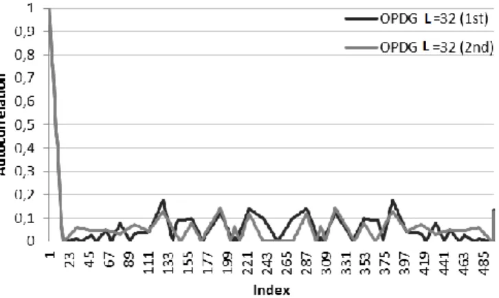
Figure 11: Normalized absolute periodic autocorrelation – OPDG codes, with a resolution of 16 bits.
Figure 11 shows the normalized periodic autocorrelation properties of the OPDG codes with the length of 32. The ACCF average is 9.48. Furthermore, by increasing the code length, autocorrelation properties (or ACCF) increase greatly. Increasing the code length of the OPDG codes results in a reduction of fluctuation in the normalized periodic autocorrelation function, as can be seen in Figure 12. This last ACCF average - 18.62 - is much higher.
Figure 12: Normalized absolute periodic autocorrelation - OPDG codes with the code length of 128, with a resolution of 16 bits
The ACCF enables us to find the better code set, and helps us minimize the MPI effect, as can be indicated by the lower amplitudes of the out-of-phase autocorrelation values in Figure 12 when compared to Figure 10 and Figure 11.
53
1.6. Standing Wave Cancellation
A common occurrence in the field of wireless communication is the standing wave. In environments that contain many obstacles, such as closed spaces, the wave that is being sent from the transmitter to the receiver propagates through space and gets reflected from different kinds of surfaces. These reflections cause the receiving end to receive multiple instances of the same wave, some of them arriving directly, while others arriving after being reflected from a certain object. This occurrence is commonly called MPI, and represents a common issue in indoor positioning systems that use wireless technology.
The MPI has another side-effect, which is called the standing wave. When a wave gets reflected from a surface, it generates another wave that propagates back in the opposite direction. If one puts a receiver somewhere between the transmitter and the reflective surface, detecting the strength of the signal would vary on the position in which the receiver is placed because of the standing wave effect. Certain positions, particularly those that are half wavelength apart, would show no oscillations in the signal strength when measured multiple times. These points along the medium are called nodes (N). Some other points along the medium would yield different results, showing high oscillations in signal strength. The points that contain the highest amount of oscillations are called the antinodes (AN) [48].
In order to achieve accurate and consistent indoor positioning estimation using signal strength, inside closed spaces, mitigating the effect of the standing wave is one of the problems that needs to be addressed. Currently, a technical solution to this problem does not exist, and as a part of this thesis, a way to solve the problem of the standing wave will be introduced, in cases where wireless communication is used in indoor positioning systems.
To solve this problem, a different kind of wireless transmitter and receiver is used within the IPS system. The functioning of this transmitters and receivers will be furtherly explained.
54
Figure 13: Standing wave cancellation
The standing wave cancellation wireless transmitter consists of a signal generator suitable for creating a signal with wavelength , an output and a relay switch, connected so that a relay switch alternatively connects the signal generator through a first path generating a first wave and through a second path to the output to generate the second wave. These two paths deliver two different signals. The first wave is created with a wavelength of , whereas the second wave is created with half the wavelength , by guiding the signal through a different path towards the output, as seen in Figure 14.
55
Figure 14: Standing Wave Cancellation - Mechanism
To generate the signal, a radio signal generator is used. The signal that the generator generates is then either sent directly to the antenna, or a relay switch (Double Pole Double Throw - DPDT) redirects the signal through a coaxial cable which has a length such as to generate a wave shifted in half the wavelength , again to the same antenna. The relay switch is then used in such a way to emit these two radio waves in time-division multiplexing, thus enabling the receiver to mitigate the effect of the standing wave by summing up the two waves before processing them.
A Portuguese patent under the number #109137 has been submitted for this mechanism. More information is available in the appendix.
56
1.7. Indoor Positioning System
In order to accurately determine the indoor position of an entity in closed space, a number of problems need to be solved. One of the problems is the MPI, which we believe can be mitigated using the OPDG codes. The other problem is the standing wave, which can be mitigated using the method described in section 1.6.
We propose a system that can use the communication of Frequency Modulation (FM) transmitters and receivers with OPDG codes to determine the indoor location of a device. The computing device we use to receive and process the codes is a small, low-powered single-board computer Raspberry Pi [49] equipped with a transceiver. A second Raspberry Pi is also used to control the transmissions of all transmitter pairs.
FM Transmitter Pair 1, OPDG 1 FM Transmitter Pair 2, OPDG 1 FM Transmitter Pair n, OPDG 1 FM Transmitter Pair n, OPDG 2 FM Transmitter Pair 1, OPDG 2 FM Transmitter Pair 2, OPDG 2 FM receiver
Figure 15: Indoor Positioning System - Network Topology
Figure 15 displays the network topology of our indoor positioning system. The topology consists of transmitters and receivers (both built with the Raspberry Pi computers).
57
Raspberry Pi
The Raspberry Pi is a low cost, credit-card sized computer developed with the intention of promoting the teaching of basic computer science in schools. Taking its size into consideration, it is a capable device that enables people of all ages to explore computing, and to learn how to program, as well as getting started with all kinds of electronics projects. It is capable of doing everything you would expect a desktop computer to do, from browsing the internet and playing high-definition video, to making spread sheets, word-processing, and playing games, and much more.
It was developed by The Raspberry Pi Foundation [49] (a charity association) and is manufactured through licensed manufacturing deals with Newark element14, RS Components and Egoman. These companies sell the Raspberry Pi online.
The form factor of the Raspberry Pi can be seen in Figure 16 below.
Figure 16: The Raspberry Pi
Due to the available resources, we have used two different model of the Raspberry Pi. The first model, Model B, can be seen on the left of the figure, while the second model, Model B+ can be seen on the right.
Raspberry Pi’s have been used as both the receivers, as well as the transmitters inside the IPS system.
58
FM Receiver
It has been mentioned that the Raspberry Pi will be used as a computing device in order to process the FM signals it receives from the transmitters in order to determine its indoor position. In order to use the Raspberry Pi as a computing device for the received FM signal, we need some kind of way to receive the FM signal and forward it to the Raspberry Pi for further processing. Out-of-the-box, the Raspberry Pi does not offer any way of receiving a FM signal. Hence, in order to receive the FM signal, an external receiver should be used.
In this case, a cheap FM tuner evaluation board was bought online and used to receive the signal. The SparkFun FM Tuner Evaluation Board (Si4703) [50] is an evaluation board that enables us to tune into FM radio stations. It breaks out all the major pins and makes it easy to incorporate the chip as a part of a bigger project. The board is powered by 3.3V, which matches the output of the Raspberry Pi’s general-purpose input/output (GPIO) pins and makes a great match with the Raspberry Pi. The board, displayed in Figure 17, also allows us to tune and seek for FM signals using a few built-in GPIO pins. By plugging the headphones into the 3.5 mm jack, we can effectively use the headphones cable as an antenna for the receiver.
Figure 17: Si4703 FM Tuner
In order to forward the signal from the FM module to the Raspberry Pi, we have used a male-to-male 3.5 mm jack cable, as displayed in Figure 18. One end of the cable was connected to the 3.5 mm female port on the FM module, while the other end was connected to the Mic input of an
59 external USB soundcard. This external sound card was connected via USB to the Raspberry Pi, since out-of-the-box the Raspberry Pi does not feature any audio input ports.
Figure 18: FM receiver module
Figure 18 also shows all the components that make up the receiver. These components are: 1. Raspberry Pi
2. External sound card
3. Si4703 FM receiver module 4. 3.5 mm jack cable
5. Power supply
The receiver would be usually powered through a USB 3.0 port on a laptop, since both the laptop and the receiver have to be carried around when performing measurements around a scenario. The Si4703 module was connected to the Raspberry Pi using the connections seen in Figure 19 below.
1
2
3
2
4
2
5
2
2
2
60
Figure 19: Si4703 to Raspberry Pi connection
FM Transmitter
Now that we have the hardware of the receiver set up, we need to set up the transmitters. In order to add functionality and modularity to the FM transmitter, we have opted to, again, use the Raspberry Pi’s.
One of the features that was not originally intended for the Raspberry Pi was the transmission of radio signals. Using a piece of code [51] hacked together at Code Club, it is possible to turn the Raspberry Pi into an FM transmitter. By connecting a short piece of wire to the GPIO 4 (GPCLK0) pin of the Raspberry Pi, and running the piece of code, you effectively get a FM transmitter.
Since the code is written in Python, it is easy to expand the functionality of the FM transmitter by adding mode features to the code, which is exactly what has been done in this case. Functionality to start/stop the receiver remotely has been included, as well as a few tweaks that help us build the IPS scenario.
61
Figure 20: FM Transmitter
The transmitter, displayed in Figure 20, consists of the following parts: 1. Raspberry Pi
2. Antenna 3. Power supply
The antenna of the transmitter can be any piece of wire. In this case, we used a 35 cm long piece of copper wire.
Control Software
In order for the system to work seamlessly, we need to connect all the nodes (receivers and transmitters) into a coherent system. To see that all of our tests for the IPS scenario have been successful, we need to find a way to monitor and control all the nodes.
While testing this software and different measurement mechanisms, there were many iterations of the software as well. For the simplicity of explaining, only the software for one scenario will be explained.
1
2
2
2
3
2
62 Since this software requires communication between the transmitters and the receiver. We have to make sure that all the transmitters and the receiver are connected to the same network, and that the receiver software has all the IP addresses of the transmitters defined.
Figure 21: IPS - simplified scenario
Figure 21 above displays a scenario in which most of the tests were performed, and the software for this scenario will be explained.
The software will be divided into two parts: Transmitter software
Receiver software
1.7.4.1. Transmitter software
As mentioned, in order to make the Raspberry Pi transmitters emit radio signals, a piece of code developed by Code Club PiHack was used as a base, after which it was upgraded to meet the needs of the IPS scenario.
63
Figure 22: Transmitter software flowchart
Figure 22 shows the flowchart that explains the way the transmitter communicates with the receiver. The transmitter waits for the signal from the receiver to know when it needs to start emitting the OPDG code. The signal is received through a Transmission Control Protocol (TCP) connection between the transmitters and the receiver.
1.7.4.2. Receiver software
The second part of the system is the receiver. Functions of the receiver are the following: Controls the transmitters (start/stop signaling) using TCP;
64
Figure 23: Receiver software flowchart
Figure 23 shows the flow of functions in the implementation of the receiver. After requesting some initial information from the user (amount of measurements, etc.) it starts capturing the FM signal coming from the transmitters.
Following the initial setup, the control software opens TCP communications towards the transmitters. It then uses this TCP communication to signal the transmitters when to transmit. The message sequence can be seen in Figure 24 below.
65
Figure 24: TCP Communication - Transmitter to Receiver
After the measurements start, at the end of each measurement the receiver is moved to a different position (due to a lack of available equipment). For each of these positions, it calculates the ratio of OPDG1/OPDG2 codes which are transmitted on only 2 transmitters at a time. The process of calculating the ACCF ratios is shown in Figure 25 below.
Figure 25: ACCF Ratio calculation
This part uses raw audio and reference codes (text files with signal amplitudes defined) to calculate the ACCF ratios. First it extracts the peaks from the correlation of the two signals. After extracting the signals, it uses the formula for the autocorrelation crest factor (defined in the Methodology section) to calculate the ACCF of each of the codes (OPDG1 and OPDG2). Finally, it calculates the ratio between the two signals and stores it.
66 After all the positions were measured, it exports the results into an Excel file. From this Excel file we can then further process the information and create some graphs to see the results.
67
Setting up
This section will deal with how the indoor positioning system was set up. The instructions will be laid out step by step and each of the steps explained.
Things we need:
5x Raspberry Pi 5x USB WiFi dongle 4x 5V power supply 4x antenna
1x external sound card
1x SparkFun FM Tuner Evaluation Board (Si4703) 1x 3.5mm jack cable
68
1.8. Transmitters
Setting up the transmitters is pretty simple and straightforward. The setup will be divided into multiple parts.
Hardware
The transmitter contains the elements explained in 1.7.3. The antenna has to be connected to the Pin 7 on the Raspberry Pi GPIO header, as displayed in Figure 26.
Figure 26: FM Transmitter - Antenna connection
In order to establish the communication between the transmitter and the receiver, they need to be connected to the same network.
Software
The software package for the transmitter contains the following: PiFm binary (“pifm”)
PiFm source code (“pifm.c”)
Transmitter program (“transmitter.py”)
Audio (WAV) files of the OPDG1 and OPDG2 codes
To set up the transmitter, continue with the following steps:
1. Transfer the files from the transmitter folder to the Raspberry Pi. Files can be transferred over the network (using Secure Copy – SCP or SSH File Transfer Protocol – SFTP) or using removable media (Universal Serial Bus – USB flash drive, etc.). Transfer them to the folder
~/transmitter.
69 2. The Raspberry Pi should come preinstalled with Python 3.x. If that is not the case, make sure it is installed with the following commands:
sudo apt-get update
sudo apt-get install python3
3. Run the transmitter script:
sudo python3 ~/transmitter/transmitter.py <wav_file>
An example would be:
sudo python3 ~/transmitter/transmitter.py OPDG1_N128_c4_x256.wav
At this point, the script is running, and our transmitter is waiting for the signal from the receiver on when it should transmit the code. This concludes setting up the transmitter.
70
1.9. Receiver
As with the transmitters, we will divide the setup of the receiver into hardware and software.
Hardware
The receiver contains the elements described in 1.7.2. Before setting up the software, make sure that the receiver’s hardware components are connected in a proper manner, as described in 1.7.2.
Software
The software package for the receiver contains the following: Receiver program (“receiver.py”)
Configuration file (“config.cfg”)
Textual representations of the amplitudes in audio (WAV) files of the OPDG1 and OPDG2 codes from the transmitter – Reference file
To set up the receiver, continue with the following steps:
1. Transfer the files from the receiver folder to the Raspberry Pi. Files can be transferred over the network (SCP, SFTP) or using removable media (USB flash drive, etc.). Transfer them to the folder ~/receiver.
2. The Raspberry Pi should come preinstalled with Python 3.x. If that is not the case, make sure it is installed with the following commands:
sudo apt-get update
sudo apt-get install python3
3. Turn on all the transmitters and make sure they are connected to the same network as the receiver.
4. Define the IP addresses of all the transmitters in config.cfg configuration file. 5. Run the transmitter script:
71
sudo python3 ~/receiver/receiver.py <reference_file_1> <reference_file_2>
An example would be:
sudo python3 ~/receiver/receiver.py OPDG1.txt OPDG2.txt
73
Tests
To test out our IPS system, a number of real-world indoor scenarios were set up, starting with a simple scenario with two transmitters, and then moving to the 2D scenario with four transmitters.
1.10. Linear scenario tests
For the first scenario, we placed two FM transmitters at a defined distance away from each other. Each transmitter was transmitting one code from a code pair on the frequency of 106.9 MHz, which has been chosen to minimize the problem of MPI due to the absence of commercial FM radio transmitters in the measurement zone. The receiver, a Raspberry Pi with a FM receiver module, was moved from one transmitter to the other, and measurements were taken at specific interval lengths. Measurements were made by simultaneously calculating the ACCF for both codes in the pair, after which a ratio was made between the two obtained values in order to cancel the FM automatic gain control. In Figure 27, the dots in between the transmitters denote the positions of the measurements taken.
Figure 27: Linear scenario
The transmitters transmit their signals in two ways: Simultaneous;
74 The test scenarios will cover both of the approaches, after which the best approach will be used for further testing.
Test scenario 1
Table 1 below displays the parameters of this test scenario.
Table 1: Test scenario 1 - Parameters
Distance between transmitters 10 meters
Code families tested OPDG
Measurements taken every 1.25 meters
Emitting type Simultaneous
Antenna length 0.15 m
Figure 28: Test scenario 1 - Results
Results gained in this first scenario, displayed in Figure 28, show the potential of the ACCF, and how it can be used to estimate the location of the receiver between two transmitters.
If we take into account the trend line of the actual results (y), we can see that the ratio of the two ACCFs slowly drops as we move from the first to the second antenna (0 to 10 m). Using the equation of the trend line y, we are able to give a rough estimation of the receiver between the two transmitters. y = -0.0188x + 1.0644 0.8 0.9 1 1.1 1.2 0 1.25 2.5 3.75 5 6.25 7.5 8.75 10 A CCF1/ A CCF2 ratio Distance (m) Average Linear (Average)
![Figure 4: Wifarer [27]](https://thumb-eu.123doks.com/thumbv2/123dok_br/18568274.907121/36.918.293.624.475.880/figure-wifarer.webp)
![Figure 5: IndoorAtlas [29]](https://thumb-eu.123doks.com/thumbv2/123dok_br/18568274.907121/37.918.143.777.391.755/figure-indooratlas.webp)


![Figure 9: Autocorrelation vs. Cross-correlation [39]](https://thumb-eu.123doks.com/thumbv2/123dok_br/18568274.907121/45.918.266.659.124.407/figure-autocorrelation-vs-cross-correlation.webp)