Local territorial reform and regional spending efficiency

REM WORKING PAPER SERIES

Local territorial reform and regional spending efficiency

REM Working Paper 071-2019

February 2019

REM – Research in Economics and Mathematics

Rua Miguel Lúpi 20, 1249-078 Lisboa,

Portugal

ISSN 2184-108X

Any opinions expressed are those of the authors and not those of REM. Short, up to two paragraphs can be cited provided that full credit is given to the authors.

1

Local territorial reform and regional spending

efficiency

António Afonso

_{, Ana Venâncio}

February 2019

Abstract

We investigate the effect of a local territorial reform, which reduced the number of parishes, on municipality spending efficiency in the period 2011-2016. We build a composite output indicator and use Data Envelopment Analysis (DEA) to compute efficiency scores, which we then analyze through a second stage regression with socio-demographic, economic factors and the reform. We find efficiency gains for around 10% of municipalities overall. In Alentejo and in Centro, more than 50% of the municipalities improved efficiency. The second stage results show that the reform did not improve local spending efficiency in Mainland Portugal, particularly in the Norte region.

JEL: C14, H72, R50.

Keywords: public spending efficiency, local government, data envelopment analysis (DEA), local

organizational reform.

* _{The opinions expressed herein are those of the authors and not necessarily those of their employers.}

$ _{ISEG – School of Economics and Management, Universidade de Lisboa; REM – Research in Economics and}

Mathematics, UECE. UECE – Research Unit on Complexity and Economics is supported by Fundação para a Ciência e a Tecnologia. email: aafonso@iseg.utl.pt.

# _{ISEG/ULisbon – University of Lisbon, Department of Management; ADVANCE – Centro de Investigação Avançada}

1. Introduction

Improving the efficiency and effectiveness of public services and at same time reducing public spending has become an important concern in the public sector. Undoubtedly, local governments could benefit from adhering to these objectives. Decentralization has transferred to the local government a considerable amount of government spending and decision-making. Yet, the resources to fulfill the demand for more and better local public services are scarce. Therefore, reforms that reduce local public spending and improve efficiency are very relevant. Most reforms have focused on two main areas: merging administrative regions or decentralizing the administrative and fiscal responsibilities. In this study, we will focus on the first type of reform.

Previous studies have evaluated the optimal size of municipalities (Doumpos and Cohen, 2014) and assessed the effect size, in terms of population, on municipality efficiency. Most studies find that efficiency scores are higher for larger municipalities (Balaguer-Coll, Prior and Tortosa-Ausina, 2007; Doumpos and Cohen, 2014) because of increasing economies of scale. Indeed, there is reasonable agreement that the smaller municipalities have higher costs (or compromised service quality) for all public services. For example, research of small local governments in Swiss Cantons suggests that costs and quality are severely compromised below a population of 500 (Ladner et al. 2003).

This paper contributes to this literature by assessing the changes on municipal efficiency stemming from a structural reform that reduced the number of administrative and local government units. Our example took place in 2013 when Portugal decreased (by around 29%) the number of parishes. Portugal provides an excellent case study to analyze the impact of this reform on municipality efficiency for three reasons. First, between 2011 and 2016, a municipality in Portugal spent on average 26 million Euros and municipality transfers to parishes accounted for approximately 4.3 percent of those expenditures. Although local governments have fiscal and

administrative autonomy, they rely heavily on funds from central government. On average, transferences from central government accounted for 42 percent of the total revenues. With this reform, the government intended to reduce the municipality spending and the amount of transfers to parishes, together with the assumption of fostering scale economies. Second, municipalities have to comply with the same rules and legislation but local politicians have some discretionary power on how to implement their policies and to use their resources. Finally, the local territory reform resulted from the memorandum of understanding signed between the Portuguese government, the EU and with the International Monetary Fund. Therefore, the need to reduce public expenditure in the local government made measuring their efficiency even more pressuring.

Hence, this study uses a two-stage methodology to measure the impact of the reform on the municipality efficiency. In the first stage, efficiency scores are measured using Data Envelopment Analysis (DEA) for the years 2011 (before the reform) and 2016 (after the reform). To compute the DEA efficiency scores, we use a composite indicator of municipal services’ provisions (outputs), as in Afonso and Venâncio (2016), and we use local government spending as the input. A second stage is proposed where the effect of the reform on the change of the efficiency scores obtained from the first stage is evaluated. We test our approach for the case of Portugal, both for the mainland and for the European Union Nomenclature of Territorial Units for Statistics (NUTS) regions.

Our results show that: i) between 2011 and 2016 there were efficiency gains for a small percentage of the municipalities, 10% and 6% respectively for the input and for the output oriented efficiency scores; ii) regionally, notably in Alentejo and in Centro, more than 50% of the municipalities improved efficiency; iii) the efficiency gains were negatively related to the territorial reform and to the reduction of parishes in mainland Portugal and particularly in Norte region.

The organization of the paper is as follows. Section 2 reviews the related literature. Section 3 reviews the Portuguese local government sector and Sector 4 presents the methodology. Section 5 reports and discusses the empirical results. Section 6 concludes.

2. Related Literature

Public finance theory argues that fiscal decentralization can increase the efficiency in the allocation of (public) resources. In other words, lower tiers of governments are closer to citizens and might provide informational advantages regarding their preferences (Ezcurra and Rodríguez-Pose, 2009). However, sometimes sub-national governments may not be able to make optimal resource allocation, since the central government usually commands more sophisticated technical resources. Therefore, the measurement of public sector efficiency and its determinants has been the subject of a growing literature.

Generally, this literature assesses technical efficiency (a concept stemming from Farrell, 1957) by using frontier analysis. Therefore, and to assess the efficiency of government spending, many studies usually estimate non-parametrically a production function frontier and derive efficiency scores based on the relative distances of inefficient observations from the frontier.1

Efficiency is measured in an input-output perspective, in which the services provided (outputs) by the local or the central government are assessed against the resources employed (inputs). Formally, the higher the ratio of outputs to inputs, the more efficient the local or the central government is.

Previous studies have used frontier techniques (data envelopment analysis, free disposal hull, stochastic frontier analysis) to analyze the cost efficiency of public sector in different

1 _{There are several parametric and non-parametric methodologies to compute technical efficiency. Parametric}

approaches include corrected ordinary least squares and stochastic frontier analysis (SFA). Among the non-parametric techniques data envelopment analysis (DEA) and free disposal hull (FDH) have been widely applied in the literature

countries or in a cross-country setup. The related literature follows broadly two streams: studies that evaluate the overall efficiency of the services provided by the (local) government, and studies that focus on a particular (municipal) public service.

Afonso et al. (2005, 2010) studied the overall public sector efficiency across several OCDE countries, taking into account the level of general government spending. On the other hand, several specific government functions such as education and health have been addressed by Afonso and St. Aubyn (2006, 2011). St. Aubyn et al. (2009) studied the case of Universities in the European Union. Overall, those studies show the existence of room for improvement regarding public spending efficiency. Although cross-country aggregated efficiency studies are very useful to compare the performance of different countries, efficiency analyses of individual countries take into account the institutional, cultural, political and economic setting providing more insights for the policy makers (Mandl, Dierx and Ilzkovitz, 2008).

Conversely, public spending efficiency studies covering the aggregated performance of local governments have been done for several countries. For instance, Van den Eeckaut, Tulkens and Jamar (1993), De Borger et al. (1994) and De Borger and Kerstens (1996, 2000) for Belgium; Athanassopoulos and Triantis (1998) and Doumpos and Cohen (2014) for Greece; Worthington (2000) for Australia; Prieto and Zofio (2001), Balaguer-Coll, Prior-Jiménez and Vela-Bargues (2002) and Benito, Bastida and Garcia (2010) for Spain; Afonso and Scaglioni (2007) and Storto (2015) for Italy; Waldo (2001) for Sweden; and Sampaio and Stosic (2005) for Brazil. In Portugal, we highlight the studies of Afonso and Fernandes (2006, 2008), Cruz and Marques (2014) and Afonso and Venâncio (2016).2 _{Other stream of research includes studies that evaluate the efficiency}

of a specific municipality service, such as Bouckaert (1992) for the fire service; Lozano, Villa and

Adenso-Dias (2004) for recycling operations and Rogge and De Jaeger (2013) for solid waste collection. Once again, the results of these two strands of the literature point to the fact that governments can attain efficiency gains at the municipal level as well.

Finally, research efforts have been also devoted to understand the major determinants of local government efficiency. Particularly, researchers have investigated the impact on municipality efficiency of a number of socio-demographic and economic characteristics, financial resources, environmental issues not controlled by the decision-makers, economies of scale and scope.

Our study aims to contribute to the local public spending literature by evaluating a specific reform, which merged several parishes in the belief that the aggregation of smaller administration entities would reduce public expenditure, and improve efficiency because of increasing economies of scale (Fox & Gurley, 2006; Warner, 2012). There are several examples where the pooling of resources, notably for water supply, sewage provision, primary education, increase efficiency notably by cost reduction. Interestingly, such pooling of resources could be dependent on the percentage of parishes, within a municipality.

3. Portuguese local government sector

To better frame the empirical results, we review some stylized facts about the Portuguese local government sector and the 2013 territorial organizational reform.

According to the Portuguese Constitution, local administration includes administrative regions, municipalities and civil parishes.3 _{As the administrative regions have not yet been}

3 _{Portugal’s administrative regions are organized into three tiers: districts and two autonomous regions of Azores and}

Madeira, municipalities and civil parishes. For statistical purposes, the European Union (EU) redefined the Portuguese territory into Nomenclature of Territorial Units for Statistics (NUTS) regions. The NUTS system subdivides the country into three levels: NUTS I (Portugal mainland and 2 autonomous regions of Azores and Madeira), NUTS II (7 regions) and NUTS III (30 sub-regions). These latter classifications were developed for the purpose of delivering structural funds for less favored regions and sub-regions.

established, the authorities responsible for delivering local public services are municipalities and parishes. At the end of 2012, there were 308 municipalities subdivided into 4,260 parishes. Of the total, 278 municipalities and 4,050 sections of municipalities, parishes, were located in mainland Portugal and the remaining 30 municipalities and 210 parishes were located in Azores and Madeira islands. In this study, we will focus on mainland municipalities and parishes because the islands have a different institutional and economic context.

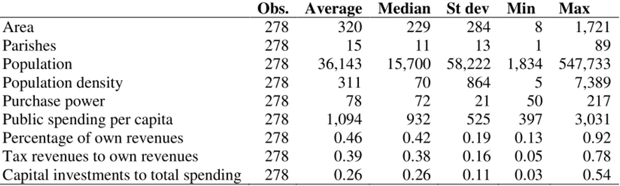
The mainland municipalities are very heterogeneous in terms of population, geographical size, purchasing power and support received from the central government. Table 1 presents the socio-demographic, economic and political characteristics of the municipalities for the year 2011.

[Table 1]

The size of municipalities varies considerably. The median was 15,700 inhabitants, and the mean was 36,143 inhabitants. Almost 45 percent of the population lives in 23 municipalities with more than 100,000 inhabitants (8 percent of all municipalities). In terms of population density, the average and median was 311 and 70 inhabitants per squared kilometers, respectively. Municipalities are also economically different. There are a few very rich municipalities. In fact, only 34 municipalities have a purchase power higher than 100.

Local governments are territorially based organizations with administrative and fiscal autonomy. They have their own employees, patrimony and fiscal independence and its activity satisfies the local needs of their citizens. While municipalities have a major role on delivering local public services to citizens, parish competences are limited to a few public services (e.g. road and park maintenance; social facilities for children and the elderly and residence permits). Nonetheless, parishes establish an important link between municipalities and citizen needs. Municipalities

provide a plethora of traditional local government services:4 _{development and maintenance of local}

infrastructures (e.g. sport, leisure and basic school facilities), supply of public goods such as drinking water, waste and sewage collection, education, childcare support, urban transportation, urban planning, health services, housing, cultural activities and events, and civil protection.5 _To

provide these local public services, municipalities can freely choose their governance structures (direct, indirect, public, private or mix). In terms of revenues, municipalities are funded with transfers from the central government, transfers from the European Union, local taxes and sales and other revenues. Nonetheless, transferences from central government account, on average, for 42 percent of the total revenues. Municipalities obtain 46 percent of their revenues by self-generated revenues and taxes account on average for 39 percent of their own revenuers. Note that municipalities cannot set their own taxes and, the rates have to be defined within a range defined centrally.6 _{Under the local finances legal framework, municipalities have their own budgets, and}

are subject to restrictive expenditure control mechanisms. They have to comply with strict budget rules and debt limits. Hence, their financial autonomy is rather limited in terms of revenues and borrowing.

In 2011, due to the sovereign debt crisis, Portugal applied for a bailout program with the International Monetary Fund, the European Central Bank and the European Commission. The memorandum of understanding signed in May 2011 entailed several clauses concerning the local government, namely: increase decentralization, reduce transfers from the central government,

4 _{Some essential services are provided by the central government or private sector. Education is a competence of the}

central governement. Electricity, natural gas, postal services, broadband and telecomincations are provided by private companies.

5 _{See Law 159/99 and Law 2/2007.}

6 _{The central government sets the tax base of all the local taxes, and the tax rate on transfers of real estate (IMT –}

Imposto Municipal sobre as Transmissões Onerosas de Imóveis). In the remaining local taxes, the municipalities set

the tax rates within a range defined at the national level. For municipal corporate income tax (Derrama) and personal income tax, municipalities cannot charge more than the maximum threshold, and for property tax (IMI – Imposto

enhance reporting on budget execution and improve efficiency of local administration. In September 2011, the Green Paper on the reform of the local administration was published and it set the following goals: accomplish effective decentralization of local services, rationalize local government structures, envisage higher proximity and efficiency of local public services and reduce the number of parishes. This reform intended to create efficiencies and reduce public spending. At the same time, it affected the territorial geography and the political management of municipalities and parishes. These changes were implemented before the local government elections of 2013. Besides reducing the number of representatives in the local boards, the reform also increased, reduced or merged various parishes within municipalities, changed the territorial limits of the parishes within municipalities, and transferred parishes from one municipality to another.7 _{Table A.1 of Appendix A presents the type of changes that occurred on each municipality.}

In addition, it is possible to observe that between 2009 and 2012, the number of parishes was 4,050. After 2013, the number of parishes reduced to 2,882, corresponding to a decrease of 29%. Of the total number of parishes, 50% merged with other parishes within the municipality (2022 parishes), 49% did not experience any change and the remaining 1% had their territorial limits changed.

Before 2013, a municipality included on average 15 parishes (see Table 2). Barcelos was the municipality with the most parishes (89 before 2013 and 61 after 2013). Four municipalities, Alpiarça, Barrancos, São Brás de Alportel and São João da Madeira, included a single parish. After 2013, Castanheira de Pera was also included to the list of municipalities with just one parish.

[Table 2]

7 _{There were two transferences of parishes between municipalities. Pombalinho parish moved from Santarém}

municipality to Golegã municipaliy. Parque das Nações parish was created including parts of the Loures municipality and Lisbon municipality.

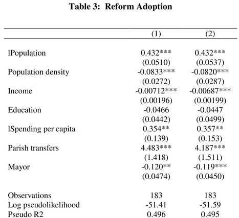
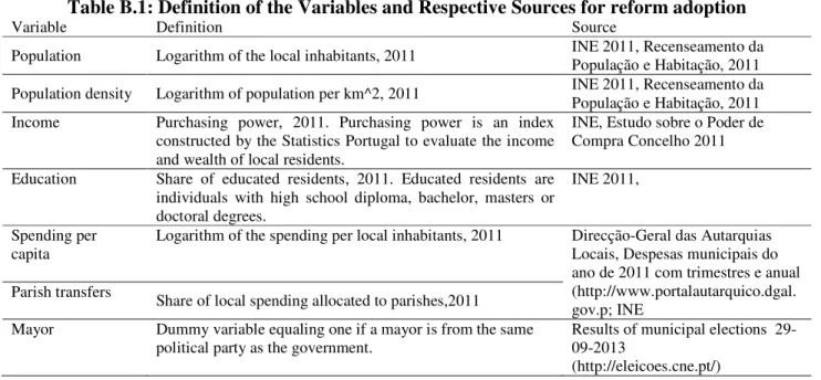
As a complementary exercise, we report in Table 3 the determinants that have contributed to the adoption of the reform. The dependent variable is a binary variable that assumes one for the municipalities that reduced the number of parishes and zero otherwise. The variable definition and sources in Appendix Table B.1. Interestingly, the likelihood of implementing the reform and reduced the number of parishes increases notably with the size of the municipality (population) and the level of per capita spending, and decreases with the level of purchasing power. The reform targeted less rich municipalities and those with larger transfers to parishes. In terms of political variables, municipalities whose mayor was from the same political party as the central government were less likely to implement the reform and reduce the number of parishes.

[Table 3]

4. Methodology

DEA is a non-parametric frontier methodology, which draws from Farrell’s (1957) seminal work and was further developed by Charnes, Cooper and Rhodes (1978). Non-parametric techniques do not require the definition of the production functions and demand fewer requirements from the data. Frontier methodologies compare all observations with the “best practices”. The production frontier in the DEA approach uses linear programming methods and computes the relative efficiency of a group of Decision Management Units (DMUs) that consume identical inputs and produce identical outputs.8 _{For each municipality i, we consider is the following function:}

) ( i i f X

Y = , i=1,…,n (1)

where Yi is the composite output measure for municipality i and Xi is the per capita municipal

expenditures registered on municipal accounts for the each year (2011 and 2016) as a measure of the municipal resources used in local services’ provision input in municipality i.

If Y_i < f X( _i), it is said that municipality i exhibits inefficiency. For the observed input levels, the actual output is smaller than the best attainable one and inefficiency is measured by computing the distance to the theoretical efficiency frontier.

Adopting an input orientation, for explanation purposes, and assuming the presence of variable-returns to scale (VRS), the efficient scores are computed through the following linear programming problem: 9 , s. to 0 0 1' 1 0 i i Max y Y x X n δ λθ θ λ λ λ λ − + ≥ − ≥ = ≥ . (2)

In this formulation, there are k inputs used to produce m outputs for n DMUs. For the i-th DMU, xi

is the column vector of the inputs and yi is the column vector of the outputs. We can also define X

as the (k×n) input matrix and Y as the (m n) output matrix.

In (3), ߠ is a scalar (that satisfies 1/ ߠ ≤ 1), and specifically is the efficiency score that measures technical efficiency, the distance between a municipality and the efficiency frontier, defined as a linear combination of the best practice observations. With 1 ߠൗ < 1 , the municipality is inside the frontier (i.e. it is inefficient), while ߠ = 1 implies that the municipality is on the frontier (i.e. it is efficient).

9 _{This is the equivalent envelopment form, derived by Charnes et al. (1978), using the duality property of the multiplier}

form of the original programming model.

The vector λ _{is a (n 1) vector of constants that measures the weights used to compute the} location of an inefficient DMU if it were to become efficient, and n1 is an n-dimensional vector of ones. The inefficient DMU can theoretically be on the production frontier as a linear combination of those weights, related to the peers of the inefficient DMU. The peers are other DMUs that are more efficient, and used as references for the inefficient DMU. The restriction _n1'λ =1 imposes

convexity of the frontier, accounting for VRS. Dropping this restriction would amount to admit that returns to scale were constant.

Problem (3) is solved for each of the n DMUs in order to obtain the n efficiency scores. The VRS scores represent the pure technical efficiencies (PTE) and take into account that fact that DMUs might not operate at the optimal scale. In contrast, scores obtained through constant return to scale (CRS) represent technical efficiency (TE) and assumes that all DMUs are operating at the optimal scale.

5. Empirical Analysis 5.1. Data and variables

The data sample used in this analysis includes 278 municipalities for two periods: 2011, before the reform and 2016, after the reform (see Table 2). Between 2011 and 2016, the Portuguese economy was influenced by several economic events, such as the financial bailout, the outbreak of the economic crisis that spanned from 2008 until 2014 and the economic recovery from 2014 onwards.

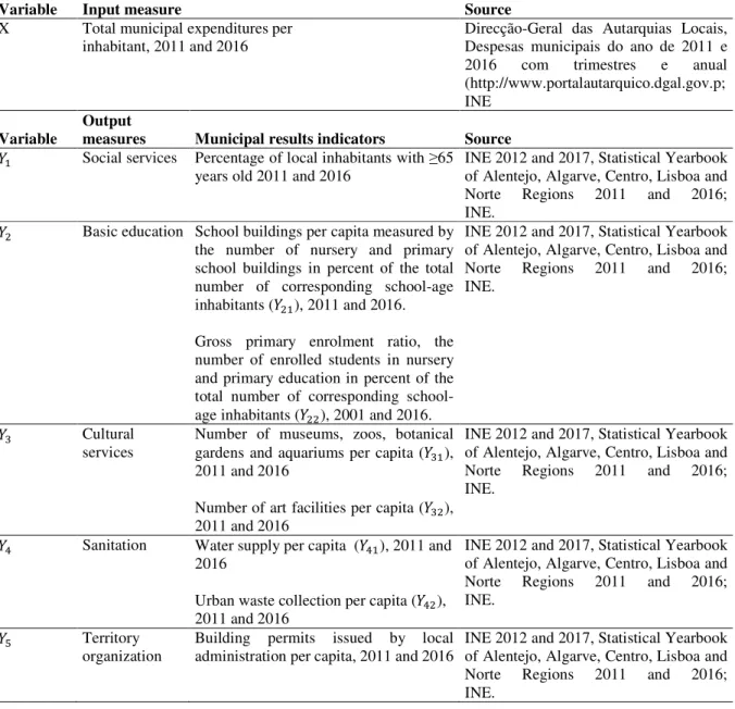
To build the DEA efficiency scores for 2011 and 2016, we construct an output composite indicator, Local Government Output Indicator (LGOI) as suggested by Afonso and Venâncio (2015). This composite is a single measure of municipal performance evaluated in terms of social

services, Y1 (local inhabitants above 65 years old as a percentage of resident population); basic education Y2 (school buildings per capita measured by the number of nursery and primary school buildings in percent of the total number of corresponding school-age inhabitants, Y21; and gross primary enrolment ratio, the number of enrolled students in nursery and primary education in percent of the total number of corresponding school age inhabitants, Y22); cultural services, Y3 (number of museums, zoos, botanical gardens and aquariums as a percentage of resident population, Y31; and number of art facilities as percentage of resident population, Y32); sanitation, Y4 (water supply per resident population, Y41; and urban waste collection per resident population, Y42); territorial organization, Y5 (building permits issued by local administration per resident population). To obtain the composite output indicator all values of each previous sub-indicator were normalised by setting the average equal to one. To compile the indicator from the various sub-indicators, we give equal weight to each of them. Our input measure includes municipal spending per resident population. Table B.2 in the Appendix B summarizes the definitions of our input and output variables and its sources.

5.2. DEA efficiency scores

Table 4 provides a summary of the DEA results that we have obtained for 2011 and 2016. The purpose of an input-oriented assessment is to study by how much one can proportionally reduce input quantities without changing the output quantities produced. Alternatively, and by computing output-oriented measures, one can assess how much output quantities can be proportionally increased without changing the input quantities used. In the case of the efficiency scores for 2011, we can see from Table 4 that input efficiency scores range between 0.514 for the Mainland and 0.674 in Algarve and in the Lisboa and Vale do Tejo (LTV) regions, implying that inputs could be theoretically lower by around 33%-49%, keeping the same level of output. On the

other hand, output efficiency scores range between 0.293 for the Mainland and 0.670 the Norte region, which means that one might envisage and output increase of around 37%-71% with the same level of inputs.

[Table 4]

Turning to the results obtained for 2016, also in Table 4, we find that the input efficiency scores range between 0.425 for the Mainland and 0.655 in Alentejo and in the Centro regions, implying that inputs could be theoretically lower by around 34%-56%, keeping the same level of output. In terms of the output efficiency scores, these range between 0.217 for the Mainland and the Alentejo region, and 0.646 for the Algarve region, implying that theoretically output could increase around 35%-78% with the same level of inputs.

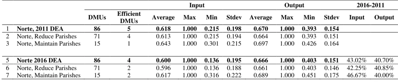
Table 5 compares with more detail the changes in the efficiency scores between 2011 and 2016 for the overall Mainland. One can notice that between 2011 and 2016 there were efficiency gains for a small percentage of the municipalities, 10% and 6% respectively for the input and for the output oriented efficiency scores. In addition, Table 6 provides a similar exercise per region. In this case, the regions where there was a higher percentage of municipalities that increased their respective efficiency scores were the Alentejo (input) and Centro (input and output) regions with more than 50% of the municipalities improving efficiency.

[Table 5] [Table 6]

5.3. Explaining efficiency

Since several exogenous factors are necessarily responsible for the existence of inefficiencies, we can then assess how the change of the efficiency scores relates to such determinants. As examples of such causes, we can consider the local territorial reform under

analysis, and factors proposed in the literature on local government efficiency, namely municipality characteristics not controlled by the mayor, changes in municipality characteristics and local governments’ discretion behavior. For that purpose, we compare the DEA input efficiency scores before and after the reform using the following equation:

∆ߠ௜ = ߚ଴ + ߚଵ∆ܲܽݎ݅ݏℎ௜ + ܼ௜′ߚଶ+ ߝ௜ (3) where i denotes inland municipality.

Our dependent variable in Equation (3), ∆ߠ_௜, is the difference between the DEA input scores before and after reform computed in the previous section.

Our variable of interest is ∆ܲܽݎ݅ݏℎ௜, defined as the change in the number of parishes within a municipality, computed as the difference between the logarithm of the number of parishes after and before the reform. Alternatively, we consider a binary variable ܴ݂݁݋ݎ݉_௜, which equals one if a municipality reduced the number of parishes, and zero otherwise. In these analyzes, we exclude one municipality which increased its number of parishes due to the reform. Our results do not change when we compute the effect of the reform in all mainland municipalities.

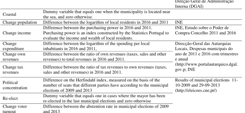
Local performance may be influenced by municipality characteristics and changes in the municipality characteristics. Therefore, we include a vector, ܼ_௜ to control for changes on sociodemographic and economic characteristics of the municipality. First, we include a binary variables coastal that equals one for municipality located near the sea and zero otherwise. This variable allow us to control for factors not influenced by the mayor namely, the existence of natural resources (beaches) and the type of geography of the municipality.

In addition, we consider the change in size of the municipality as the difference between the logarithm of local residents in 2016 and 2011. According to Grossman et al. (1999), the monitoring costs to mitigate local government’s discretional behavior increase with geographic ‘scarcity of

municipalities’. Hence, there might be scale economies regarding local public services provision. In addition, richer local residents usually impose higher pressure for more efficient services,10 _we

therefore include the change in income/wealth measured as the change in the purchasing power in 2016 and 2011.

To control for the change on financial characteristics of the municipality, we include the

change on spending per capita, measured as the change of the total public expenses per

inhabitants in 2016 and 2011; the change on financial independence, measured as the change in the ratio of own revenues (taxes, sales and other revenues) to total revenues in 2016 and 2011; and the change on tax revenues to own revenues ratio in 2016 and 2011. Overreliance on central government funds is related to inefficiencies in municipalities (De Borger et al., 1993). The change on tax revenues to own revenues ratio is employed to take into account the change on the level of municipalities on tax collection. As taxes do not correspond to a specific array of services, contrary to revenues from services provisions, municipalities that increase their share could be characterized as less successful on providing chargeable services.

To capture local governments tendency to pursue their self-interests and their political agenda (Niskanen, 1975; Migué and Bélanger, 1974), we include three political variables: first, we use the Herfindahl index to assess the political concentration in the council of each municipality, measured based on the number of seats that different parties have according to the municipal elections of 2009 and 2013. A decrease (an increase) in political concentration from 2009 to 2013 suggests that the concentration of political power is getting weaker (stronger) and the opposition party is getting stronger (weaker), which may have a negative efficiency impact. The greater the variety of viewpoints the more intense the decision-making process. A stronger political leadership

may have more power in internal bargain and may find it more likely to resist the pressure to accommodate low efficiency and lower outputs (Borge, 2008). We also introduce a dummy variable, re-elect, that equals one in cases where the mayor has been re-elected in the last municipal elections and zero otherwise. Re-elected mayors for a second-term may be less motivated to implement policies towards improving the quantity and quality of services provided to citizens. The change on voter turnout is computed as the change in the abstention rate in municipal elections. The definition and sources of the explanatory variables are presented in Table B.3 of Appendix B.

The results from Table 7 show that several determinants contribute to explain the efficiency scores in the case of the full Mainland sample. The reform itself, taken as binary determinant, shows that reducing the number of parishes within a municipality actually contributes to a decrease in the input efficiency score (see Column 3 in Table 7). In addition, using the actual changes in the number of parishes (Columns 1 and 2 in Table 7), the results display an input efficiency reduction effect. A 10% reduction on the number of parishes implies a decrease of 0.01 in efficiency. In terms of control variables, the increase of population and of government expenditure, diminish efficiency as well. In contrast, an increase on own revenues ratio and tax revenues ratio is associated with efficiency increases. In terms of political variables, a reduction on voter turnout, increases efficiency as well.

[Table 7]

Form a regional perspective, we find (see Table 8) that the overall results for the Mainland case essentially hold. This is specially the case of Norte region. However, in the Alentejo and Algarve region (panel D in Table 8), the reduction in the number of parishes (accounting for control variables) does increase the input efficiency scores. This result yet does not hold, when we use a dummy variable for reform.

[Table 8]

Our results are no too different, although less robust, when the analysis is performed in terms of output efficiency scores. In addition, we used different estimation methods – Tobit and a double bootstrap procedure. These estimation models show similar results as the OLS regressions. Additionally, we controlled for several external factors (i.e. tourism index, area, population density, automobile fuel consumption, energy consumption, mayor, left and right wing) that might affect efficiency. Nonetheless, we removed the non-significant variables and those that presented Variance Inflation Factors (VIF) over 10. All these results available upon on request.

5. Conclusion

To evaluate if a territorial reform had a positive effect on the change on the efficient scores between 2011 and 2016 in Portugal, we used DEA approach. We computed the DEA efficiency scores using a composite output indicator of municipal services’ provision, and we use municipal expenditure per inhabitant, in 2011 and in 2016 as the input. Afterwards, we assessed through a second stage regression whether socio-demographic and economic factors and the reform explained the change on efficiency.

Our results can be summarized as follows: i) overall, there are input and output efficiency gains for around 10% and 6% of municipalities, respectively; ii) regionally, notably in Alentejo and in Centro, more than 50% of the municipalities improved efficiency; iii) nevertheless, the second stage results show that the territorial reform did not improve local spending efficiency in mainland Portugal and particularly in the Norte region; The results are similar for the case of the output efficiency scores.

From a policy perspective, it is then less obvious that such reform, which implied a reduction of the number of parishes, has enhanced the efficiency of government spending across the board for the municipalities. Indeed, efficiency increases only in some regions, and policy makers need to account for such specific characteristics. Importantly, reforms like the one evaluated in this study require efforts between the central and local governments. Central government initiatives for improving local service efficiency and public spending can only be effective if local governments are willing participants in those reforms. In fact, local governments have to be motivated to implement those reforms on their own because they know more closely the needs of their citizens and how to improve the services provided.

The current study has its limitation. First, there is the issue of selecting inputs and outputs to compute the efficiency score and the selection of the control variables for the second-stage analysis. Even though the choice relied on the services provided by the local government defined in the legal framework, other authors could have chosen different variables, naturally also limited to data availability. The same applies to the control variables in the second-stage estimation. Finally, this study draws on data from the local government of one country naturally raising questions about the generalizability of these findings to another geographic context. While we make no claims that our findings are perfectly generalizable to other countries, the theoretical underpinnings of our model provide a framework for exploring these phenomena in other geographic locations.

References

Afonso, A., Fernandes, S. (2006). “Measuring local government spending efficiency: Evidence for the Lisbon Region”. Regional Studies 40 (1), 39-53.

Afonso, A., Fernandes, S. (2008). “Assessing and explaining the relative efficiency of local government”, Journal of Socio-Economics 37 (5), 1946–1979.

Afonso, A., Scaglioni, C. (2007). “Efficiency in Italian regional public utilities’ provision”, in

Servizi Publici: Nuove tendenze nella regolamentazione, nella produzione e nel finanziamento,

pp. 397-418, eds. M. Marrelli, F. Padovano and I. Rizzo, 2007, Franco Angeli, Milano, Italy. Afonso, A., St. Aubyn, M. (2006). “Cross-country Efficiency of Secondary Education Provision:

a Semi-parametric Analysis with Non-discretionary Inputs”, Economic Modelling, 23 (3), 476-491.

Afonso, A., St. Aubyn, M. (2011). “Assessing health efficiency across countries with a two-step and bootstrap analysis”, Applied Economics Letters, 18(15), 1427-1430.

Afonso, A., Schuknecht, L., Tanzi, V. (2005). “Public Sector Efficiency: An International Comparison”, Public Choice, 123 (3-4), 321-347.

Afonso, A., Schuknecht, L., Tanzi, V. (2010). “Public Sector Efficiency: Evidence for New EU Member States and Emerging Markets”, Applied Economics, 42 (17), 2147-2164.

Athanassopoulos, A., Triantis, K. (1998). “Assessing Aggregate Cost Efficiency and the Related Policy Implications for Greek Local Municipalities”, INFOR, 36(3), 66-83.

Balaguer-Coll, M, Prior-Jimenez, D., Vela-Bargues, J. (2002). “Efficiency and Quality in Local Government Management. The Case of Spanish Local Authorities”, Universitat Autonoma de Barcelona, WP 2002/2.

Charnes, A.; Cooper, W., Rhodes, E. (1978). “Measuring the efficiency of decision making units”,

European Journal of Operational Research, 2, 429–444.

Coelli T., Rao, D., Battese, G. (2002). An Introduction to Efficiency and Productivity Analysis, 6th

edition, Massachusetts, Kluwer Academic Publishers.

De Borger, B., Kerstens, K., Moesen, W., Vanneste, J. (1994). “Explaining differences in productive efficiency: An application to Belgian Municipalities”, Public Choice, 80 (3-4), 339-358.

De Borger, B., Kerstens, K. (1996). “Cost efficiency of Belgian local governments: A comparative analysis of FDH, DEA, and econometric approaches”, Regional Science and Urban Economics, 26, 145-170.

De Borger, B., Kerstens, K. (2000). “What Is Known about Municipal Efficiency?” In Blank, J., Lovell, C. and Grosskopf, S. (eds). Public Provision and Performance – contributions from

efficiency and productivity measurement. Amsterdam, North-Holland, 299-330.

Dorn, D. (2009). “Essays on Inequality, Spatial Interaction, and the Demand for Skills” Dissertation of the University of St. Gallen, Graduate School of Business Administration, Economics, Law and Social Sciences (HSG).

Eugène, B. (2008). “The efficiency frontier as a method for gauging the performance of public expenditure: a Belgian case study”, National Bank of Belgium, WP 138.

Farrell, M. (1957). “The Measurement of Productive Efficiency”, Journal of the Royal Statistical

Society Series A (General), 120, 253-281.

Grossman, P., Mavros, P., Wassmer, R. (1999). “Public Sector Technical Inefficiency in Large U.S. Cities”, Journal of Urban Economics, 46 (2), 278–299.

Hamilton, B. (1983). “The Flypaper Effect and Other Anomalies”, Journal of Public Economics, 22 (3), 347–361.

Hayes, K., Razzolini, L., Ross, L. (1998). “Bureaucratic Choice and Nonoptimal Provision of Public Goods: Theory and Evidence”, Public Choice, 94, 1–20.

Migué, J., Bélanger, G. (1974). “Toward a General Theory of Managerial Discretion”, Public

Choice, 17, 27–43.

Niskanen, W. (1975). “Bureaucrats and Politicians”, Journal of Law and Economics, 18 (3), 617– 643.

Prieto, A., Zofio, J. (2001). “Evaluating Effectiveness in Public Provision of Infrastructure and Equipment: The Case of Spanish Municipalities“, Journal of Productivity Analysis, 15 (1), 41-58.

St. Aubyn, M., Pina, A., Garcia, F., Pais, J. (2009). “Study on the efficiency and effectiveness of public spending on tertiary education”, Economic Papers 390, European Commission.

Thanassoulis, E. (2001). Introduction to the Theory and Application of Data Envelopment Analysis. Kluwer Academic Publishers.

Tolbert, C., Killian, M. (1987). “Labor Market Areas for the United States.”Staff Report No. AGES870721. Washington, DC: Economic Research Service,US Department of Agriculture. Tolbert, C., Size, M. (1996). “U.S. Commuting Zones and Labor Market Areas. A 1990

Update.”Economic Research Service Staff Paper No. 9614.

Van den Eeckhaut, P., Tulkens, H., Jamar, M.-A. (1993). “Cost-efficiency in Belgian municipalities,” in Fried, H.; Lovell, C. and Schmidt, S. (eds.), The Measurement of Productive Efficiency: Techniques and Applications. New York: Oxford Univ. Press.

Worthington, A. (2000). “Cost Efficiency in Australian Local Government: A comparative analysis of mathematical programming and econometric approaches”, Financial Accounting and

Table 1: Municipalities socio-demographic and economic characteristics (2011)

Obs. Average Median St dev Min Max

Area 278 320 229 284 8 1,721

Parishes 278 15 11 13 1 89

Population 278 36,143 15,700 58,222 1,834 547,733

Population density 278 311 70 864 5 7,389

Purchase power 278 78 72 21 50 217

Public spending per capita 278 1,094 932 525 397 3,031

Percentage of own revenues 278 0.46 0.42 0.19 0.13 0.92

Tax revenues to own revenues 278 0.39 0.38 0.16 0.05 0.78

Capital investments to total spending 278 0.26 0.26 0.11 0.03 0.54

Table 2: Some stylized facts for the municipalities

2011 2016 2016-2011 Number of parishes 4,050 2,882 -28.84% Number of municipalities 278 278 0.00% Reduce parishes 230 Maintain parishes 47 Increase parishes 1 Resident population 10,047,621 9,809,414 -2.37% Reduce parishes 9,481,635 9,250,040 -2.44% Maintain parishes 560,521 553,866 -1.19% Increase parishes 5,465 5,508 0.79%

Average population per km^2 311 303 -2.52%

Reduce parishes 341 332 -2.74%

Maintain parishes 169 169 -0.38%

Increase parishes 71 65 -7.90%

Average purchasing power 78.0 80.8 3.62%

Reduce parishes 77.7 80.5 3.62%

Maintain parishes 79.7 82.5 3.54%

Increase parishes 78.4 83.3 6.27%

Average spending per capita 1,094 1,055 -3.59%

Reduce parishes 1,041 1,005 -3.51%

Maintain parishes 1,351 1,296 -4.00%

Increase parishes 1,154 1,172 1.59%

Average share of transfers to parishes 2.79% 3.32% 0.53%

Reduce parishes 3.13% 3.70% 0.58%

Maintain parishes 1.11% 1.44% 0.32%

Increase parishes 0.03% 2.67% 2.63%

Note: The table reports some stylized facts for the local government sector for the years 2011 and 2016 by municipalities that reduced, maintained or increased the number of parishes. Column “2016-2011” reports the percentage change between those years.

Table 3: Reform Adoption (1) (2) lPopulation 0.432*** 0.432*** (0.0510) (0.0537) Population density -0.0833*** -0.0820*** (0.0272) (0.0287) Income -0.00712*** -0.00687*** (0.00196) (0.00199) Education -0.0466 -0.0447 (0.0442) (0.0499)

lSpending per capita 0.354** 0.357**

(0.139) (0.153) Parish transfers 4.483*** 4.187*** (1.418) (1.511) Mayor -0.120** -0.119*** (0.0474) (0.0450) Observations 183 183 Log pseudolikelihood -51.41 -51.59 Pseudo R2 0.496 0.495

Note: Columns (1) and (2) report the marginal coefficients using probit and logit models, respectively. The dependent variable is a dummy variable equalling one if a municipality experienced a reduction in the number of parishes. The definition and sources of the independent variables are presented in Table B.1 of Appendix B. Districts dummies are included but not reported. Standard errors clustered at the district level are in parentheses. *** denotes statistical significance at 1%, ** significance at 5%, * significance at 10%.

25

Table 4: DEA Efficiency Results

2011 2016

Efficient DMUs Average efficiency

scores Efficient DMUs

Average efficiency scores Region N. of DMUs N. of DMUs (municipality) % of DMUs in the region Input oriented Output

oriented N. of DMUs (municipality)

% of DMUs in the region Input oriented Output oriented

Alentejo 47 3 (Beja, Elvas, Sines) 6.38% 0.622 0.596 3 (Beja, Santiago do Cacém, Sines) 6.38% 0.655 0.217 Algarve 16 4 (Alcoutim, Faro, _{Olhão, Tavira)} 25.00% 0.674 0.628 3 (Alcoutim, Olhão, Tavira) 18.75% 0.611 0.646 Centro ₇₈ 4 (Anadia, Vila do

Rei, Gouveia, Leiria) 5.13% 0.636 0.603 3 (Vila do Rei, Gouveia, Leiria) 3.85% 0.655 0.629

LVT 51

3 (Caldas da Rainha,Almada,

Tomar) 5.88% 0.674 0.452 2 (Sintra, Tomar) 3.92% 0.615 0.386 Norte 86

5 (Macedo de Cavaleiros, Vila Flor,

Valongo, Vila Nova de Gaia, Alijó)

5.81% 0.618 0.670 _{Cavaleiros, Vila Flor, Valongo)} 4 (Barcelos, Macedo de 4.65% 0.600 0.666 Mainland 278 2 (Tomar, Valongo) 0.72% 0.514 0.293 3 (Monchique,Tomar, Valongo) 1.08% 0.425 0.217 Note: The table reports the DEA efficiency scores using 2011 and 2016 data. The column “Efficient DMUs” reports the number and name of efficient DMUs and the percentage of efficient municipalities in a region. DMUs is Decision Management Units.

Table 5: DEA Country Efficiency Scores Comparisons (VRS)

Input Output 2016-2011

DMUs Efficient

DMUs Average Max Min Stdev Average Max Min Stdev Input Output

1 Country, 2011 DEA 278 2 0.514 1.000 0.185 0.197 0.293 1.000 0.140 0.115

2 Country, Reduce Parishes 230 1 0.509 1.000 0.185 0.197 0.291 0.922 0.140 0.109

3 Country, Maintain Parishes 47 1 0.544 1.000 0.198 0.194 0.297 1.000 0.177 0.128

4 Country, Increase Parishes 1 0 0.223 0.223 0.223 0.000 0.684 0.684 0.684 0.000

5 Country, 2016 DEA 278 3 0.425 1.000 0.065 0.181 0.217 1.000 0.112 0.093 10.07% 6.12%

6 Country, Reduce Parishes 230 1 0.416 1.000 0.065 0.177 0.210 0.595 0.112 0.065 10.00% 5.65%

7 Country, Maintain Parishes 47 2 0.474 1.000 0.213 0.185 0.248 1.000 0.127 0.171 10.64% 8.51%

8 Country, Increase Parishes 1 0 0.128 0.128 0.128 0.000 0.254 0.254 0.254 0.000 0.00% 0.00%

Note: The table reports the input and output DEA efficiency scores for the mainland Portugal for the years 2011, Rows (1) to (4), and 2016, Rows (5) to (8). Rows

(1) and (5) report the scores for the 278 municipalities, Rows (2) and (6) report the scores for the municipalities that reduced the number of parishes, Rows (3) and (7) report the scores for the municipalities that maintained the number of parishes, and the remaining rows report the scores for the municipalities that increased the number of parishes. The column “Efficient DMUs” reports the number of efficient DMUs and the column “2016-2011” reports the percentage of cases (municipalities) where there is a gain in efficiency, by comparing the 2011 efficiency score of the municipalities and the 2016 efficiency score.

Table 6: DEA Regional Efficiency Scores Comparisons (VRS)

Input Output 2016-2011

DMUs Efficient

DMUs Average Max Min Stdev Average Max Min Stdev Input Output

1 Norte, 2011 DEA 86 5 0.618 1.000 0.215 0.198 0.670 1.000 0.393 0.154

2 Norte, Reduce Parishes 71 4 0.613 1.000 0.215 0.194 0.664 1.000 0.393 0.151

3 Norte, Maintain Parishes 15 1 0.643 1.000 0.301 0.215 0.697 1.000 0.426 0.164

5 Norte 2016 DEA 86 4 0.600 1.000 0.136 0.195 0.666 1.000 0.403 0.151 43.02% 40.70%

6 Norte, Reduce Parishes 71 2 0.596 1.000 0.136 0.188 0.661 1.000 0.403 0.146 42.25% 40.85%

7 Norte, Maintain Parishes 15 2 0.617 1.000 0.316 0.222 0.689 1.000 0.451 0.175 46.67% 40.00%

Input Output 2016-2011

DMUs Efficient

DMUs Average Max Min Stdev Average Max Min Stdev Input Output

1 Centro 2011 DEA 78 4 0.636 1.000 0.223 0.201 0.603 1.000 0.187 0.172

2 Centro, Reduce Parishes 63 4 0.636 1.000 0.223 0.210 0.601 1.000 0.187 0.183

3 Centro, Maintain Parishes 15 0 0.637 0.850 0.267 0.157 0.614 0.862 0.445 0.112

5 Centro, 2016 DEA 78 3 0.655 1.000 0.175 0.183 0.629 1.000 0.187 0.171 53.85% 56.41%

6 Centro, Reduce Parishes 63 3 0.646 1.000 0.175 0.192 0.620 1.000 0.187 0.181 52.38% 52.38%

7 Centro, Maintain Parishes 15 0 0.691 0.917 0.463 0.133 0.667 0.872 0.461 0.116 60.00% 73.33%

Input Output 2016-2011

DMUs Efficient

DMUs Average Max Min Stdev Average Max Min Stdev Input Output

1 LVT 2011 DEA 51 3 0.674 1.000 0.343 0.193 0.452 1.000 0.237 0.155 2 LVT, Reduce Parishes 41 2 0.669 1.000 0.354 0.199 0.444 0.939 0.237 0.145 3 LVT, Maintain Parishes 10 1 0.693 1.000 0.343 0.165 0.483 1.000 0.263 0.186 5 LVT, 2016 DEA 51 2 0.615 1.000 0.281 0.170 0.386 1.000 0.195 0.166 39.22% 0.00% 6 LVT, Reduce Parishes 41 1 0.608 1.000 0.281 0.175 0.377 0.801 0.195 0.150 41.46% 0.00% 7 LVT, Maintain Parishes 10 1 0.644 1.000 0.454 0.145 0.421 1.000 0.202 0.217 30.00% 0.00%

Input Output 2016-2011

DMUs Efficient

DMUs Average Max Min Stdev Average Max Min Stdev Input Output

1 Alentejo, 2011 DEA 47 3 0.622 1.000 0.343 0.166 0.596 1.000 0.279 0.182

2 Alentejo, Reduce Parishes 41 2 0.619 1.000 0.343 0.156 0.592 1.000 0.279 0.171

3 Alentejo, Maintain Parishes 6 1 0.642 1.000 0.424 0.224 0.620 1.000 0.334 0.238

5 Alentejo, 2016 DEA 47 3 0.655 1.000 0.192 0.170 0.530 1.000 0.279 0.171 61.70% 14.89%

6 Alentejo, Reduce Parishes 41 2 0.650 1.000 0.192 0.168 0.536 1.000 0.279 0.176 63.41% 17.07%

7 Alentejo, Maintain Parishes 6 1 0.687 1.000 0.556 0.180 0.484 0.592 0.291 0.116 50.00% 0.00%

Input Output 2016-2011

DMUs Efficient

DMUs Average Max Min Stdev Average Max Min Stdev Input Output

1 Algarve, 2011 DEA 16 4 0.674 1.000 0.437 0.213 0.628 1.000 0.377 0.201

2 Algarve, Reduce Parishes 14 3 0.664 1.000 0.437 0.204 0.607 1.000 0.377 0.189

3 Algarve, Maintain Parishes 1 0 0.487 0.487 0.487 0.000 0.549 0.549 0.549 0.000

4 Algarve, Increase Parishes 1 1 1.000 1.000 1.000 0.000 1.000 1.000 1.000 0.000

5 Algarve, 2016 DEA 16 3 0.611 1.000 0.374 0.243 0.646 1.000 0.367 0.218 6.25% 31.25%

6 Algarve, Reduce Parishes 14 2 0.599 1.000 0.374 0.230 0.629 1.000 0.367 0.210 7.14% 35.71%

7 Algarve, Maintain Parishes 1 0 0.400 0.400 0.400 0.000 0.532 0.532 0.532 0.000 0.00% 0.00%

8 Algarve, Increase Parishes 1 1 1.000 1.000 1.000 0.000 1.000 1.000 1.000 0.000 0.00% 0.00%

Note: The tables report the input and output DEA efficiency scores for the Norte, Centro, Lisboa and Vale do Tejo, Alentejo and Algarve

region for the years 2011, Rows (1) to (4), and 2016, Rows (5) to (8). Rows (1) and (5) report the scores for the total number of municipalities within a region, Rows (2) and (6) report the scores for the municipalities that reduced the number of parishes, Rows (3) and (7) report the scores for the municipalities that maintained the number of parishes, and the remaining rows report the scores for the municipalities that increased the number of parishes. The column “Efficient DMUs” reports the number of efficient DMUs and the column “2016-2011” reports the percentage of cases (municipalities) where there is a gain in efficiency, by comparing the 2011 efficiency score of the municipalities and the 2016 efficiency score. DMUs is Decision Management Units. Max is maximum, Min is minimum and Stdev is standard deviation.

29

Table 7: Regression Model for the Change on Municipality Efficiency Scores

(1) (2) (3) (4) Change parishes 0.157*** 0.084** (0.032) (0.034) Reform -0.043*** -0.032 (0.013) (0.020) Coastal 0.009 0.007 (0.007) (0.007) Change population -0.330** -0.284* (0.153) (0.164) Change income 0.210 0.246* (0.132) (0.146) Change expenditure -0.354*** -0.359*** (0.041) (0.042) Change own revenues 0.172** 0.175** (0.085) (0.085) Change tax revenues 0.102** 0.103** (0.044) (0.047) Political concentration 0.015 0.021

(0.060) (0.060)

Re-elect 0.008 0.008

(0.012) (0.011) Change voter turnout -0.002** -0.003***

(0.001) (0.001) Constant -0.015 -0.085*** -0.025** -0.079***

(0.009) (0.014) (0.011) (0.019) District dummies Yes Yes Yes Yes

Observations 277 277 277 277

Sigma 0.096*** 0.067*** 0.098*** 0.067*** (0.010) (0.015) (0.010) (0.015) Log likelihood 255.0 357.4 249.8 356.5

Note: The table reports the estimated coefficients for Equation (3) using tobit regression model. The dependent variable is the change in DEA input scores between 2016 and 2011. The definition and sources of the independent variables are presented in Table B.3 of Appendix B. Standard errors clustered at the district level are in parentheses. *** denotes statistical significance at 1%, ** significance at 5%, * significance at 10%.

Table 8: Regression Results for the Change on Regional Municipality Efficiency Scores

(1) (2) (3) (4) (1) (2) (3) (4)

Panel A: Norte Region Panel B: Centro Region

Change parishes 0.157* -0.039 _{Change parishes} 0.020 0.076

(0.087) (0.056) (0.076) (0.048)

Reform _{-0.008*** -0.044*** Reform} 0.016 0.006

(0.000) (0.015) (0.034) (0.022)

Sigma 0.107*** 0.038*** 0.108*** _{0.038*** Sigma} 0.106*** 0.045*** 0.106*** 0.046*** (0.009) (0.005) (0.009) (0.006) (0.017) (0.004) (0.017) (0.004) Log likelihood 70.12 159.1 69.08 159.2 _{Log likelihood} 64.67 131.8 64.74 130.0

Panel C: LVT Region Panel D: Alentejo e Algarve Regions

Change parishes 0.125 0.053 _{Change parishes} 0.029 -0.124***

(0.092) (0.049) (0.074) (0.030)

Reform 0.029 0.020 _Reform -0.017 -0.040***

(0.036) (0.031) (0.014) (0.010)

Sigma 0.088*** 0.043*** 0.091*** _{0.043*** Sigma} 0.104*** 0.042*** 0.104*** 0.042*** (0.009) (0.004) (0.012) (0.004) (0.015) (0.004) (0.016) (0.004) Log likelihood 50.58 86.18 49.06 85.81 _{Log likelihood} 53.08 110.3 53.20 109.9

Note: The table reports the estimated coefficients for Equation (3) using tobit regression model. The dependent variable is the change in DEA regional input scores between 2016 and 2011. Panel A, B, C and D present the coefficients results separately for Norte, Centro, Lisbon and Vale do Tejo and Alentejp and Algarve regions, respectively. The number of observations for Panel A, B, C and D equals 86, 78, 50 and 63, respectively. Columns (1) and (3) do not include control variables and Columns (2) and (4) add control variables. The definition and sources of the independent variables are presented in Table B.3 of Appendix B. All models include district dummies fixed effects. Standard errors clustered at the district level are in parentheses. *** denotes statistical significance at 1%, ** significance at 5%, * significance at 10%.

31

Appendix

Appendix A – 2013 Territorial Reform Table A.1: Type of changes

Parishes 2011 Parishes 2016 Municipality No change Merged Changed

limits Transferred Eliminated New Total Total

Abrantes 8 11 19 13 Águeda 4 16 20 11 Aguiar da Beira 7 6 13 10 Alandroal 3 3 6 4 Albergaria-a-Velha 4 4 8 6 Albufeira 3 2 5 4 Alcácer do Sal 3 3 6 4 Alcanena 5 5 10 7 Alcobaça 9 9 18 13 Alcochete 3 3 3 Alcoutim 3 2 5 4 Alenquer 6 10 16 11 Alfândega da Fé 6 14 20 12 Alijó 10 9 19 14 Aljezur 4 4 4 Aljustrel 3 2 5 4 Almada 1 10 11 5 Almeida 9 20 29 16 Almeirim 4 4 4 Almodôvar 4 4 8 6 Alpiarça 1 1 1 Alter do Chão 4 4 4 Alvaiázere 3 4 7 5 Alvito 2 2 2 Amadora 11 11 6 Amarante 18 22 40 26 Amares 11 13 24 16 Anadia 7 8 15 10 Ansião 5 3 8 6 Arcos de Valdevez 23 28 51 36 Arganil 10 8 18 14 Armamar 10 9 19 14 Arouca 12 8 20 16 Arraiolos 3 4 7 5 Arronches 3 3 3

Arruda dos Vinhos 4 4 4

Aveiro 7 7 14 10 Avis 4 4 8 6 Azambuja 6 3 9 7 Baião 8 12 20 14 Barcelos 43 46 89 61 Barrancos 1 1 1 Barreiro 1 7 8 4 Batalha 4 4 4

Parishes 2011

Parishes 2016 Municipality

No

change Merged Changed limits Transferred Eliminated New Total Total

Beja 6 12 18 12 Belmonte 3 2 5 4 Benavente 4 4 4 Bombarral 3 2 5 4 Borba 4 4 4 Boticas 5 11 16 10 Braga 18 44 62 37 Bragança 31 18 49 39 Cabeceiras de Basto 8 9 17 12 Cadaval 4 6 10 7 Caldas da Rainha 8 2 6 16 12 Caminha 9 11 20 14 Campo Maior 3 3 3 Cantanhede 9 10 19 14 Carrazeda de Ansiães 10 9 19 14 Carregal do Sal 4 3 7 5 Cartaxo 4 4 8 6 Cascais 2 4 6 4 Castanheira de Pêra 2 2 1 Castelo Branco 13 12 25 19 Castelo de Paiva 4 5 9 6 Castelo de Vide 4 4 4 Castro Daire 11 11 22 16 Castro Marim 4 4 4 Castro Verde 3 2 5 4 Celorico da Beira 12 10 22 16 Celorico de Basto 10 12 22 15 Chamusca 3 4 7 5 Chaves 29 19 3 51 39 Cinfães 13 4 17 14 Coimbra 8 23 31 18 Condeixa-a-Nova 4 6 10 7 Constância 3 3 3 Coruche 5 3 8 6 Covilhã 14 17 31 21 Crato 3 3 6 4 Cuba 4 4 4 Elvas 3 8 11 7 Entroncamento 2 2 2 Espinho 3 2 5 4 Esposende 4 11 15 9 Estarreja 3 4 7 5 Estremoz 5 8 13 9 Évora 6 13 19 12 Fafe 17 19 36 25 Faro 2 4 6 4 Felgueiras 12 20 32 20 Ferreira do Alentejo 2 4 6 4 Ferreira do Zêzere 3 2 4 9 7 Figueira da Foz 7 4 7 18 14 Figueira de Castelo Rodrigo 5 12 17 10

Parishes 2011

Parishes 2016 Municipality

No

change Merged Changed limits Transferred Eliminated New Total Total

Figueiró dos Vinhos 3 2 5 4

Fornos de Algodres 9 7 16 12

Freixo de Espada à Cinta 2 4 6 4

Fronteira 3 3 3 Fundão 18 13 31 23 Gavião 3 2 5 4 Góis 3 2 5 4 Golegã 2 1 3 3 Gondomar 3 9 12 7 Gouveia 10 12 22 16 Grândola 3 2 5 4 Guarda 33 22 55 43 Guimarães 31 38 69 48 Idanha-a-Nova 9 8 17 13 Ílhavo 4 4 4 Lagoa 2 4 6 4 Lagos 2 4 6 4 Lamego 14 10 24 18 Leiria 9 20 29 18 Lisboa 43 10 1 53 24 Loulé 8 3 11 9 Loures 4 14 18 10 Lourinhã 5 6 11 8 Lousã 2 4 6 4 Lousada 9 16 25 15 Mação 5 3 8 6 Macedo de Cavaleiros 24 14 38 30 Mafra 6 11 17 11 Maia 7 10 17 10 Mangualde 8 10 18 12 Manteigas 4 4 4 Marco de Canaveses 6 25 31 16 Marinha Grande 3 3 3 Marvão 4 4 4 Matosinhos 10 10 4 Mealhada 5 3 8 6 Mêda 8 8 16 11 Melgaço 8 10 18 13 Mértola 6 3 9 7 Mesão Frio 4 3 7 5 Mira 4 4 4 Miranda do Corvo 3 2 5 4 Miranda do Douro 9 8 17 13 Mirandela 25 12 37 30 Mogadouro 17 11 28 21 Moimenta da Beira 13 7 20 16 Moita 2 4 6 4 Monção 17 16 33 24 Monchique 3 3 3 Mondim de Basto 4 4 8 6 Monforte 4 4 4 Montalegre 17 18 35 25

Parishes 2011

Parishes 2016 Municipality

No

change Merged Changed limits Transferred Eliminated New Total Total

Montemor-o-Novo 5 5 10 7 Montemor-o-Velho 9 5 14 11 Montijo 2 6 8 5 Mora 4 4 4 Mortágua 6 4 10 7 Moura 3 5 8 5 Mourão 3 3 3 Murça 5 4 9 7 Murtosa 4 4 4 Nazaré 3 3 3 Nelas 5 4 9 7 Nisa 5 5 10 7 Óbidos 6 3 9 7 Odemira 8 6 2 1 17 13 Odivelas 1 6 7 4 Oeiras 2 8 10 5 Oleiros 8 4 12 10 Olhão 3 2 5 4 Oliveira de Azeméis 9 10 19 12 Oliveira de Frades 5 7 12 8 Oliveira do Bairro 3 3 6 4 Oliveira do Hospital 11 10 21 16 Ourém 9 9 18 13 Ourique 2 4 6 4 Ovar 4 4 8 5 Paços de Ferreira 9 7 16 12 Palmela 3 2 5 4 Pampilhosa da Serra 6 4 10 8 Paredes 17 7 24 18 Paredes de Coura 11 10 21 16 Pedrógão Grande 3 3 3 Penacova 5 6 11 8 Penafiel 23 15 38 28 Penalva do Castelo 9 4 13 11 Penamacor 7 5 12 9 Penedono 5 4 9 7 Penela 3 3 6 4 Peniche 3 3 6 4 Peso da Régua 4 8 12 8 Pinhel 10 17 27 18 Pombal 11 6 17 13 Ponte da Barca 12 13 25 17 Ponte de Lima 30 21 51 39 Ponte de Sor 4 3 7 5 Portalegre 4 6 10 7 Portel 4 4 8 6 Portimão 3 3 3 Porto 4 11 15 7 Porto de Mós 7 6 13 10 Póvoa de Lanhoso 16 13 29 22 Póvoa de Varzim 4 8 12 7 Proença-a-Nova 2 4 6 4

Parishes 2011

Parishes 2016 Municipality

No

change Merged Changed limits Transferred Eliminated New Total Total

Redondo 2 2 2 Reguengos de Monsaraz 3 2 5 4 Resende 7 8 15 11 Ribeira de Pena 3 4 7 5 Rio Maior 6 8 14 10 Sabrosa 10 5 15 12 Sabugal 23 17 40 30 Salvaterra de Magos 2 4 6 4

Santa Comba Dão 3 6 9 6

Santa Maria da Feira 16 15 31 21

Santa Marta de Penaguião 5 5 10 7

Santarém 12 15 27 18

Santiago do Cacém 6 5 11 8

Santo Tirso 9 15 24 14

São Brás de Alportel 1 1 1

São João da Madeira 1 1 1

São João da Pesqueira 8 6 14 11

São Pedro do Sul 10 9 19 14

Sardoal 4 4 4 Sátão 7 5 12 9 Seia 14 15 29 21 Seixal 3 3 6 4 Sernancelhe 9 8 17 13 Serpa 3 4 7 5 Sertã 7 7 14 10 Sesimbra 3 3 3 Setúbal 3 5 8 5 Sever do Vouga 5 4 9 7 Silves 4 4 8 6 Sines 2 2 2 Sintra 4 16 20 11

Sobral de Monte Agraço 3 3 3

Soure 8 4 12 10 Sousel 4 4 4 Tábua 7 8 15 11 Tabuaço 9 8 17 13 Tarouca 4 6 10 7 Tavira 3 6 9 6 Terras de Bouro 11 6 17 14 Tomar 6 10 16 11 Tondela 12 14 26 19 Torre de Moncorvo 9 8 17 13 Torres Novas 6 11 17 10 Torres Vedras 7 13 20 13 Trancoso 15 14 29 21 Trofa 2 6 8 5 Vagos 5 6 11 8 Vale de Cambra 6 3 9 7 Valença 7 9 16 11 Valongo 3 2 5 4 Valpaços 20 11 31 25 Vendas Novas 2 2 2

Parishes 2011

Parishes 2016 Municipality

No

change Merged Changed limits Transferred Eliminated New Total Total

Viana do Alentejo 3 3 3 Viana do Castelo 19 21 40 27 Vidigueira 4 4 4 Vieira do Minho 11 10 21 16 Vila de Rei 3 3 3 Vila do Bispo 3 2 5 4 Vila do Conde 14 16 30 21 Vila Flor 9 10 19 14

Vila Franca de Xira 2 9 11 6

Vila Nova da Barquinha 3 2 5 4

Vila Nova de Cerveira 7 8 15 11

Vila Nova de Famalicão 23 26 49 34

Vila Nova de Foz Côa 12 5 17 14

Vila Nova de Gaia 8 16 24 15

Vila Nova de Paiva 4 3 7 5

Vila Nova de Poiares 4 4 4

Vila Pouca de Aguiar 12 6 18 14

Vila Real 12 18 30 20

Vila Real de Santo

António 3 3

3

Vila Velha de Ródão 4 4 4

Vila Verde 21 37 58 33 Vila Viçosa 3 2 5 4 Vimioso 7 7 14 10 Vinhais 18 17 35 26 Viseu 18 16 34 25 Vizela 3 4 7 5 Vouzela 6 6 12 9 Total 1972 2022 54 1 1 4050 2882

Appendix B – Variable definitions and sources

Table B.1: Definition of the Variables and Respective Sources for reform adoption

Variable Definition Source

Population Logarithm of the local inhabitants, 2011 INE 2011, Recenseamento da _{População e Habitação, 2011} Population density Logarithm of population per km^2, 2011 INE 2011, Recenseamento da _{População e Habitação, 2011} Income Purchasing power, 2011. Purchasing power is an index

constructed by the Statistics Portugal to evaluate the income and wealth of local residents.

INE, Estudo sobre o Poder de Compra Concelho 2011 Education Share of educated residents, 2011. Educated residents are

individuals with high school diploma, bachelor, masters or doctoral degrees.

INE 2011,

Spending per capita

Logarithm of the spending per local inhabitants, 2011 Direcção-Geral das Autarquias Locais, Despesas municipais do ano de 2011 com trimestres e anual (http://www.portalautarquico.dgal. gov.p; INE

Parish transfers _{Share of local spending allocated to parishes,2011} Mayor Dummy variable equaling one if a mayor is from the same

political party as the government.

Results of municipal elections 29-09-2013