Equity Research - Corticeira Amorim

M

ASTER IN

F

INANCE

M

ASTER

F

INAL

W

ORK

P

ROJECT

W

ORK

E

QUITY

R

ESEARCH

–

C

ORTICEIRA

A

MORIM

F

ÁBIO

F

ERREIRA

M

ARTINS

M

ASTER IN

F

INANCE

M

ASTER

F

INAL

W

ORK

P

ROJECT

W

ORK

E

QUITY

R

ESEARCH

–

C

ORTICEIRA

A

MORIM

F

ÁBIO

F

ERREIRA

M

ARTINS

S

M

´

:

P

D

.

I

M

G

T

F

D

F

P

Resumo

A Corticeira Amorim SGPS é líder mundial no mercado de cortiça, sendo uma empresa altamente exportadora. A sua estratégia passa por uma aposta forte em atividades de investigação e desenvolvimento e controlo de qualidade, que permitem fornecer uma qualidade diferenciadora e um leque de produtos alargado. Apesar da fraca conjuntura económica registada na Europa nos últimos anos, a empresa tem conseguido explorar novos mercados e novas tendências de modo a melhorar sustentadamente a sua rentabilidade operacional.

Este trabalho procura determinar o justo valor por acção da Corticeira Amorim, através da aplicação do método Free Cash Flow to Firm, que segundo a revisão de leitura é o mais adequado para a empresa em questão.

De acordo com os pressupostos utilizados, o valor da empresa fixa-se nos 5.59€ (por ação) o que concede ao papel um potencial de valorização de 18%, sendo atribuída uma recomendação de compra.

Abstract

Corticeira Amorim SGPS is a world leader in the cork market and a highly exporting company. Its strategy involves a strong focus on research and development and quality control activities, which provide a distinctive quality and an extended range of products. Despite the weak economic environment recorded in Europe in recent years, the company has been able to explore new markets and new trends consistently in order to sustainably improve its operating profitability.

This study seeks to determine the fair value per share of Corticeira Amorim, by applying the Free Cash Flow to Firm method, which after reading the review seems to be the most suitable for the company in question.

According to the assumptions we worked on, the company's value is fixed in 5.59 euros (per share), which gives the paper a potential appreciation of 18%, being assigned a purchase recommendation.

Table of Contents

List of Figures ... v

List of Tables ... v

List of Appendix ... vi

List of Equations ... vii

Introduction ... 1

2. Literature Review... 2

2.1. Framework ... 2

2.2. Valuation Models ... 2

2.2.1. Discounted Cash Flows ... 4

2.2.3. Relative valuation ... 9

2.2.4. Sensitivity Analysis ... 9

3. Cork Industry ... 9

3.1 Cork Industry in Portugal ... 11

4. Corticeira Amorim ... 12

4.1. Cork Cluster ... 13

4.2. CA Today ... 13

4.3. Business Areas ... 14

4.4. Revenues, Margins and Leverage ... 14

5.1 Revenues prospects per Business Units ... 19

5.1.1. Raw Materials ... 19

5.1.2. Cork Stoppers ... 19

5.1.3. Floor and Wall Coverage ... 20

5.1.4. Composite Cork ... 21

5.1.5. Insulation Cork ... 22

5.2 Operating Expenses ... 22

5.3 Gross Fixed Assets and Net Fixed Assets ... 23

5.4. Capex & Net Working Capital ... 24

5.5. WACC and Capital Structure ... 26

5.6. Terminal Value ... 28 5.11. Value of each BU ... 28 5.12. Company Valuation ... 30 5.11. Relative Valuation ... 31 5.12. Sensitivity Analysis ... 32 6. Conclusions ... 34 References ... 35 Appendix ... 40

List of Figures

FIGURE 1 - VALUATION MODELS... 3

FIGURE 2 - STRUCTURE OF CORK SALES (EXPORTS) PER PRODUCT TYPE ... 10

FIGURE 3 - TRADE BALANCE OF THE PORTUGUESE CORK INDUSTRY (CURRENT PRICES) ... 11

FIGURE 4 -HISTORICAL PRICE OF RAW CORK IN PORTUGAL (€/@ IN CELL) ; @=14,688KG ... 12

FIGURE 5 - SALES IN THOUSANDS OF EURO ... 15

FIGURE 6 - EBITDA AND EBITDA MARGIN FROM 2008-2014 ... 16

FIGURE 7 - NET DEBT AND NET DEBT/EBITDA FROM 2008-2014 ... 17

List of Tables TABLE I - SALES BREAKDOWN PER COUNTRY ... 15

TABLE II – HISTORICAL TRADE SALES BY BUSINESS UNIT IN EUROS ... 18

TABLE III–FORECASTED TRADE SALES BY BUSINESS UNIT IN EUROS ... 19

TABLE IV–HISTORICAL EBITDASPLIT PER BUSINESS UNIT ... 22

TABLE V–FORECASTED EBITDASPLIT PER BUSINESS UNIT ... 23

TABLE VI–HISTORICAL GROSS FIXED ASSETS IN EUROS ... 23

TABLE VII–FORECASTED GROSS FIXED ASSETS IN EUROS ... 23

TABLE VIII – WEIGHT OF NET FIXED ASSETS ON GROSS FIXED ASSETS ... 24

TABLE IX – HISTORICAL CAPEX BREAKDOWN BY BU ... 24

TABLE X - FORECASTED CAPEX BREAKDOWN BY BU ... 25

TABLE XI – NWC BREAKDOWN ... 25

TABLE XII – FORECASTED NWC BREAKDOWN ... 25

TABLE XIV – HISTORICAL COST OF DEBT (%) AND HISTORICAL EURIBOR (%) ... 26

TABLE XV – RAW MATERIALS ESTIMATED VALUE (THOUSANDS EURO) ... 29

TABLE XVI – CORK STOPPERS ESTIMATED VALUE (THOUSANDS EURO) ... 29

TABLE XVII - FLOOR AND WALL COVERAGE ESTIMATED VALUE (THOUSANDS EURO) ... 29

TABLE XVIII – COMPOSITE CORK ESTIMATED VALUE (THOUSANDS EURO) ... 30

TABLE XIX - INSULATION CORK ESTIMATED VALUE (THOUSANDS EURO) ... 30

TABLE XX – EQUITY VALUATION ... 31

TABLE XXI – RELATIVE VALUATION ... 32

TABLE XXII - SENSITIVITY ANALYSIS ... 33

List of Appendix APPENDIX 1 - CORK OAK FOREST AREA BY COUNTRY ... 40

APPENDIX 2-CORK OAK FOREST AREA IN PORTUGAL BY REGION IN % ... 40

APPENDIX 3–SWOTANALYSIS ... 41

APPENDIX 4-CABUSINESS UNITS ... 41

APPENDIX 5–WORLDWIDE PRESENCE ... 42

APPENDIX 6-SHAREHOLDER STRUCTURE ... 42

APPENDIX 7 - MACROECONOMIC FRAMEWORK REAL GDP ... 43

APPENDIX 8 – WEIGHT OF TRADE SALES ON TOTAL SALES ... 43

APPENDIX 9 - VINEXPO FORECASTS TO 2018: ... 43

APPENDIX 10 – TOTAL CONSTRUCTION SPENDING LONG-TERM GROWTH BY REGION (%) ... 44

APPENDIX 11 – CASH AND INTEREST BEARING LOANS ... 44

APPENDIX 13 – NET FINANCIALS COSTS AND COST OF DEBT (%) ... 45

APPENDIX 14 - FORECASTED MINORITY INTERESTS ... 46

APPENDIX 15 - HOLDING ESTIMATED VALUE (THOUSANDS EURO) ... 46

List of Equations EQUATION 1 ... 4

EQUATION 2 ... 5

EQUATION 3 ... 5

ABREVIATIONS

APT – Arbitrage Price Theory APV – Adjusted Present Value BU – Business Unit

CA – Corticeira Amorim CAPEX – Capital Expenditure

CAPM – Capital Asset Pricing Model DCF – Discounted Cash Flow

DDM – Dividend Discount Model

EBITA – Earnings Before Interests, Taxes and Amortizations

EBITDA - Earnings Before Interests, Taxes, Depreciations and Amortizations EU – European Union

EURIBOR – Euro Interbank Offered Rate EVA – Economic Value Added

FCFE – Free Cash Flow to Equity FCFF - Free Cash Flow to Firm GVA – Gross Value Added PSI – Portugal Stock Index

SGPS – Sociedade Gestora Participações Sociais TCA - Trichloroanisole

Introduction

This work has the final purpose to evaluate the company Corticeira Amorim SGPS in order to give an estimate of the intrinsic value per share on 31/12/2015. Through this analysis, we aim to attribute an investment recommendation by the comparison between the market price and the intrinsic value reached by this work. Despite the usefulness of this result, we should take into consideration that this analysis is based on assumptions and predictions that may be determinant to the results of this work and, consequently, its conclusion. In order to mitigate this risk, a sensitive analysis is performed.

Corticeira Amorim is the world cork leader, being committed with product diversification, market diversification and research and development. Except for the case of forests´ ownership, the company pursues a vertically integrated strategy that assures a full control of the production chain. The group activity is divided into 5 distinct business units accordingly to the products: raw materials, cork stoppers, floor and wall coverage, insulation cork and cork composites. Despite this diversification, the cork stoppers business continues to play a key role in the whole company business. This work is structured in six major sections. The next section presents the Literature Review that gives the theoretical framework. Section 3 and 4 give a portray of cork industry and the company´s history. Corticeira Amorim valuation is conducted in section 5 and our investment recommendation is given in the last section.

2. Literature Review

2.1. Framework

In order to clearly understand the roots of an equity research method, the first section is based on a theoretical approach. Therefore, we suggest starting with the following questions: “What is value?” and “Why assess the company´s value?”

Accordingly to Koller et al. (2010), value is a standard of performance since it takes into account the long-term interests of all the stakeholders in a company. According to the same authors, it is important to keep the valuation through time and through different scenarios and circumstances to access the impact of the company´s value. Notwithstanding, it is important to stress out that the output of any valuation method should not and cannot be perceived as an absolute truth, since it is conditioned by the assumptions that are taken into account. A much straighter response is provided by Fernandez (2007) that states the importance of valuation in company buying and selling operations: indicating the highest price the buyer should pay and, on the other hand, the lowest price at which the seller should agree to sell.

2.2. Valuation Models

The first step of a valuation is to select the most suitable method regarding the company in question. There is not a rule that states which is suitable or not, nonetheless, it is important to analyze the business specificities and it is important to compare the value between other comparable companies. Pinto et al. (2010) set the following three criteria: consistency with the company in question, suitable with the available data and consistent with goal of valuation.

Broadly speaking, we can conceive four distinct approaches: the Discounted Cash Flow valuation, the accounting and liquidation value, the Relative valuation and the Contingent Claim valuation. On Figure I, the several models are synthesized accordingly to Damodaran (2007, 2012).

Figure 1 - Valuation Models

Source: Damodaran (2007 and 2012)

Having with starting point the characteristics of Corticeira Amorim, the necessary available data for the construction of a valuation and the purpose of this work, the Discounted Cash Flow approach appears to be the most adequate. Since the model accounts for: endogenous and exogenous assumptions; the impact of the operating strategies and the possibility to value different business (Pinto et al., 2010). Additionally, a relative valuation is performed in order to have a wider perspective in

Discounted

Cash Flow

Firm Valuation Models

•Free Cash Flow to Firm •Economic Value Added Equity Valuation Models •Dividend Discount Model

•Free Cash Flow to Equity APV (Adjusted Present Value)

Accounting

and

Liquidation

value

Relative

Valuation

Contingent

Claim

Valuation

terms of valuation outputs. Besides, those valuation methods applied to the company in study, the remaining approaches and its respective methods are also covered in

Appendix 2.

2.2.1. Discounted Cash Flows

The discounted cash flow (DCF) methods are based on expected future cash flows discounted at a rate accordingly to its associated riskiness. (Cooper & Nyborg, 2006; Fernández, 2007)

Value of Assets = E(CF1) (1 + r)+ E(CF2) (1 + r)2+ E(CF3) (1 + r)3+ E(CFn) (1 + r)n (1) Whereas:

E(CFt) = Expected Cash Flow in period t

r = discount rate of each estimated cash flow n = last period of analysis

Despite these set of methods are the most used methodology in valuation firms, there is lack of consensus about its precision, since there is no guaranty that the future cash flows (and other assumptions taken into account) are accurately estimated. This may impact dramatically the valuation output (Dixit & Pindyck, 1995; Leslie & Michaels, 1997).

Accordingly to the finance literature there are several discount cash flow methodologies. This work will briefly explain the following models: Firm Valuation Models, Equity Valuation Models and Adjusted Present Value (Damodaran, 2007).

From the Discounted Cash Flow models, the most commonly used is the Free Cash Flow to the Firm (FCFF) which is discussed in the next chapter, since it will be applied on methodology.

2.2.1.1. Free Cash Flow to Firm (FCFF)

The FCFF discounts the after tax free cash flow released by operation activity at the weighted average cost of capital (WACC) which includes all types of capital: equity, debt and hybrid. Then, the claims on cash flow of debt holders and other non-equity investors are subtracted from company´s value in order to determine equity holders’ value (DePamphilis, 2010; Koller et al., 2010; Luehrman, 1997). Translating this concept mathematically comes (Fernandez 2007; DePamphilis, 2010):

𝐹𝐶𝐹𝐹 = 1 − 𝑡 ∗ 𝐸𝐵𝐼𝑇 + 𝐷𝑒𝑝𝑟𝑒𝑐𝑖𝑎𝑡𝑖𝑜𝑛𝑠 𝑎𝑛𝑑 𝐴𝑚𝑜𝑟𝑡𝑖𝑧𝑎𝑡𝑖𝑜𝑛𝑠 + ∆𝑃𝑟𝑜𝑣𝑖𝑠𝑖𝑜𝑛𝑠 − ∆𝑁𝑒𝑡 𝑊𝑜𝑟𝑘𝑖𝑛𝑔 𝐶𝑎𝑝𝑖𝑡𝑎𝑙 − 𝐶𝑎𝑝𝑖𝑡𝑎𝑙 𝑒𝑥𝑝𝑒𝑛𝑑𝑖𝑡𝑢𝑟𝑒𝑠

(2)

Note, that the depreciations, amortizations and the variation of provisions are summed to the net operational income, instead of subtracted, since are costs which do not result in outflows.

Damodaran (2007) presents the present value of expected free cash flows to the firm being computed as it follows:

𝑉𝑎𝑙𝑢𝑒 𝑜𝑓 𝑎 𝐹𝑖𝑟𝑚 = 𝐹𝐶𝐹𝐹

(1 + 𝑊𝐴𝐶𝐶)𝑡 𝑡=+∞

Where,

FCFFt = Free Cashflow to firm in year t WACC = Weighted average cost of capital

Damodaran (2007), Koller et al. (2010) and Pinto et al. (2010) argue that this model is suitable to companies with a stable capital structure, since this assures a steadier WACC during the forecasted period. The companies which do not comply with this assumption will have different WACC values during the forecasted period, since leverage influence the perception of risk for the shareholders.

Further Concepts on DCF models WACC and Capital Structure

As previously mentioned, the WACC is an average weighted by the proportion of equity and debt on capital structure, combining the cost of capital and the cost of debt. Mathematically comes:

𝑊𝐴𝐶𝐶 = 𝐸 𝐸 + 𝐷∗ 𝑘𝑒 + 𝐷 𝐸 + 𝐷∗ 𝑘𝑑 ∗ (1 − 𝑇) (4) Where,

E-Total outstanding capital D- Total outstanding debt ke cost of capital

kd cost of capital

It is plausible to think that the capital structure can drastically change thought time, changing the WACC through time. Pinto et al. (2010) and Ferris et Petitt (2002) suggest

using target weights instead of current weights. These authors refer that the target weights are the expected ones over time.

The risk free rate is the rate of return on asset with no risk at all. Damodaran (2015) states that this variable will have impact on the cost of capital, taking the assumption that the long-term government bonds are risk free assets.

The market risk premium consists in the difference on returns between a free risk asset and a riskier asset like stocks or corporate bonds (Ross et al., 2012). Damodaran (2012) stress out that this concept will have an impact on both cost of equity and cost of debt.

The beta parameter measures the sensitivity of a company in respect to its market. Thus, if beta is larger than 1, the company ends up being riskier than the market. Damodaran (2012) shows that the historical market beta can be estimated by linear regressions of corporate stocks past returns against the proper market index’s returns, representing a proxy to the true market portfolio. Blume (1971) suggests that the beta value in the future tends to the mean value of 1.0, thus the author suggest multiplying the raw beta by a weight of 2/3 and add 1 multiplied by 1/3, in order to reflect this evidence.

According to Goedhart et al. (2005) the cost of equity is estimated by the expected rate of return of the company. The asset-pricing models more often used to estimate this value are: the Capital Asset Pricing (CAPM) and Arbitrage Pricing Theory (APT). Later on, CAPM will be applied in such way that return on a stock is given by the

product of the stocks beta with market risk premium plus a rate of return in a risk free asset.

The cost of debt is a cost a company supports when borrowing money from other parties. Damodaran (2001) explains that this cost is result of: probability of default risk, level of interest rates in the market and tax deductibility associated to the interest payments. Following this train of thought, two distinct approaches are possible in order to reach an estimate to this item. The first one is only applicable to the companies that bearing long-term bonds listed in an exchange (Koller et al., 2015). If it is not the case, the cost of debt can be computed thought its historical values in order to find the pretax cost of debt. Afterwards, we apply the marginal tax rate in order to reflect the tax benefit resulting from interest (Damodaran, 2009).

Terminal Value

Damodaran (2012) explains that due to the uncertainty of futures cash flows, it is necessary to choose a time frame and then calculate the terminal value that reflects the value of the firm at that point. Subsequently, it is assumed that the firm will be facing a steady-state phase with a constant growth rate. Koller et al. (2010) recommended a time frame of 5 to 7 years while forecasting future cash flows until the terminal value, Notwithstanding sometimes it is quite difficult to determine when a company reaches that steady-state.

2.2.3. Relative valuation

Koller et al (2010) stress that with the application of the multiples, a company is able to compare its performance with the other market players. Although, the useful application of these methods, the same authors alert for the common misunderstood and misapplied of multiples, highlighting the importance of singularity of each company. Hereupon, it´s natural that, for example, two companies in the same industry, have a different P/E ratio, since they can have drastically different expected growth rates, returns on invested capital, and capital structures. Thereby Koller et al. (2010) reinforce the importance of the initial selection process of the peers, these should present similar expectations for return on invested capital and for growth. Also stressing, the multiples should not be based on historical performance but on future events, since those produce more accurate forecasts.

2.2.4. Sensitivity Analysis

Graham and Dodd (1934) stress the importance of considering a range of intrinsic values, instead of only have static values. Thus, it raises the need of performing a sensitive analysis that allows understanding what happens to a company´s value if occurs a change in some inputs.

3. Cork Industry

Despite the imprecise and non-consensual framework regarding the start of cork use or its initial main purposes, the reinvention of stoppers, in the middle ages, appears to be the booster for this material (Pestana e Tinoco, 2009). Although there are new products made by cork, there is a high exposure of the cork industry to the wine

industry. This dependence accounts for 68.4% of total sales and make France, Italy and the United States of the America, which are the key markets in wine industry (APCOR, 2013). Notwithstanding, in the last years the focus on product diversification allowed the emergence of different products and applications, in particular in the construction sector, which represents 24.5 percent of whole sales-including floors, insulation and coverings, blocks, plates, sheets, strips and other cork products (figure 1).

Figure 2 - Structure of cork sales (exports) per product type

Accordingly with ADC (2012), the cork industry can be divided by three different stages: the raw cork market, the market for intermediate cork derivates and market of final cork derivatives products, which can subdivided by gross sales and retail sales. These markets are very conditioned by the rigidity of the quantity supplied and the quality of the cork, due to: specific cork soil limitations, limited density of trees per hectare and its slow growing.

Cork oak tree is a distinctive Mediterranean tree; despite all the attempts to spread the tree around the world had failed (USA, Latin America, Russia, China and South Africa). These failed experiments were not successful in producing cork with high

42%

26% 24%

7% 1%

Natural Cork Stoppers

Other Stoppers

Floor and Wall Covering, Insulation, e tc

standards of quality that are required for industry purposes (Corticeira Amorim, 1983). Thus, Portugal appears as the leader of Cork Oak Forest area (appendix 2).

Despite the positive contribution to environment, due to the cork stripping, Demertzi et al. (2015) and González-García et al. (2015) propose some improvements in the production procedures in order to reduce the negative environmental impact in Portugal.

3.1 Cork Industry in Portugal

In Portugal, the major concentration of cork oak forest is in the Alentejo (84.1%) (Appendix 3). Being inserted in the Forestry Industry, the Portuguese Cork business represents 16% of the GVA (Gross Value Added) of this industry and 0.2% of the national GVA (INE, 2013 and APCOR, 2014). Regarding the Portuguese trade balance, figure 3 depicts a positive contribute of the cork industry thought the last years. Although, that contribute appears to have a negative trend throughout the years in analysis, mainly, due to the fall of cork average prices (Figure 3). This fall in association with the international crisis made 2009 a year of many challenges and troubles for the industry.

Figure 3 - Trade Balance of the Portuguese Cork industry (Current Prices)

0 200 400 600 800 1000 M ill ion €

Exports Imports Balance Source: APCOR Yearbook

Figure 4 - Historical Price of Raw Cork in Portugal (€/@ in cell) ; @=14,688kg

Sierra-Pérez et al. (2015) characterize the Portuguese industry as an industry that produces and process raw cork with high added value, by opposition to Spain, which is mainly composed by half manufactured cork products. Exception made to the region of Cataluña, which is the global market leader in champagne stoppers.

Lastly, it is important to explain the big challenge for the sector in the last years: Trichloroanisole (TCA). This problem consists in the appearance of the cork taint in the wines and it is the basis for the rising of synthetic stoppers in the wine market. Sefton and Simpson (2005) identify the possible factors that are in the origins of TCA as: the solubility of the taint compounds in wine, their affinity for the surface and the interior parts of the cork and the volume of wine in contact with a closure.

4. Corticeira Amorim

The Corticeira Amorim (from now on, defined as CA) birth was in 1908 with the establishment of a small workshop producing cork stoppers in Santa Maria de Lamas,

15 20 25 30 35 40 45 2002 2003 2004 2005 2006 2007 2008 2009 2010 2011 2012 2013 Pr ic e in E u ro s Source: UNAC 2014

in the north region of Portugal. In 1922, the company Amorim e Irmãos was created with the aim to export the cork stoppers, this expansion was achieved through a backward vertical integration during the next years. The official appearance of

Corticeira Amorim Lda was in 1962 with the focus on reaching foreign markets which

were considered as cork producers and, later, in cork consumer markets (Branco et al., 2014).

4.1. Cork Cluster

Branco et al. (2014) e Branco & Parejo (2011) present the importance of the cork cluster established in Santa Maria da Feira. This cluster was characterized by high specialized family nature business. Due to this, the Amorim group acquired such competitive advantages such as: lower labor costs, social networks and high degree of cooperation between the firms in the cluster. Notwithstanding, Lopes & Branco (2013) conclude that there is no empirical evidence that supports the economic advantages due to geographical concentration of cork production.

4.2. CA Today

Nowadays, the CA business model is characterized by its dominant position in the cork business; this leadership is based nearly on a 25% world market share in cork stoppers, a 80% market share in cork Insulation, 55% market share in composite cork and 65% market share in floor and wall coverage (Corticeira Amorim website).

CA business model is based on the control of the whole business production chain from raw material storage, production, distribution and sale of the final products. This vertically integrated strategy has been present in the company vision since ever and

allows the group to have a: flexibility in its production process and give a better response to different needs in the diverse markets; create entry barriers and gain competitive advantage over competitors which are mainly either producers or distributors; have a portfolio diversification that can mitigate the operational market risks and, simultaneously, adjust to the market trends and needs. In order to deeply understand the reality of CA business, a SWOT analysis is performed on the appendix 4.

4.3. Business Areas

CA is divided into five business units: Raw Materials, Cork Stoppers, Floor and Wall Coverings, Composite Cork and Insulation Cork (appendix 5).

In 2014, the company was present in more than 63 countries, with: 30 industrial units, 83 companies and 248 agents (appendix 6). Concerning the weight of sales per business units, the cork stoppers represents 60%, 22% for the Floor and Wall Coverings, the Composite cork market 15%, and 1% of the market of Insulation Cork and the rest 1% are revenues from raw materials.

4.4. Revenues, Margins and Leverage

Table I depicts that CA is a very international company, since in 2014 only 4.4% of whole revenues were generated in the Portuguese market. The high relevance of the European Union (EU) can be explained by the dependence relationship of the cork industry to the wine industry. In the chapter, France, Germany and Italy take the large share of the sales. Notwithstanding, these are very mature markets, and that is why, in the last years, CA is committed in the exploration of new markets such as USA, China

and Latin America. Actually, nowadays, USA is a key market, but it is perceived as a very compelling one, due its dimension and potential growth.

Table I - Sales Breakdown per Country

As displayed in Figure 5, the year 2009 was a very tough year. Revenues fall down by about 11% mainly due to: the crisis associated with a weak demand observed worldwide and by the gain of the market share of the synthetic stoppers, in the stoppers market. In 2009, the synthetic stoppers had a 35% of market share against a 25% market share in 2004. Nonetheless, by the end of 2014, the cork made stoppers recover its market share to 70%, due to more competitive prices and benefiting from bankruptcy of four major companies of synthetic stoppers. The sustainable growth of CA revenues can be also explained by the exploration of new products developed by R&D and new markets (mainly the USA).

Figure 5 - Sales in thousands of euro

341,459 60.9% 329,777 60.7% 24,834 4.4% 27,042 5.0% 27,310 4.9% 32,723 6.0% 107,967 19.3% 99,107 18.3% 39,104 7.0% 37,319 6.8% 35,749 6.4% 35,689 6.6% 8,750 1.6% 8,564 1.6% Africa Australasia Other American countries

United States Other European countries

2014 2013

Sales breakdown per country Europen Union From which: Portugal

Figure 6 confirms 2009 as the worst year, also in terms of EBITDA amounts, but after that year the figure depicts a general trend to growth except in 2013. In this year the fall in EBITDA is explained by the fall of EBITDA MARGIN and by unfavorable foreign exchange movements. Looking forward to 2014, the recovery of both EBITDA and EBITDA margin was mainly due to the stoppers BU, which has registered an increasing of a 13% of its own EBITDA against 2013.

Figure 6 - EBITDA and EBITDA MARGIN from 2008-2014

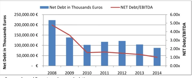
The figure 7 clearly evidenced that CA has been taking a serious commitment in reducing its levels of leverage in the last years. The company has about 66 million of

2008 2009 2010 2011 2012 2013 2014 468,289 415,210 456,790 502,344 540,979 550,265 569,953 0.0% 5.0% 10.0% 15.0% 20.0% 0 20000 40000 60000 80000 100000 2008 2009 2010 2011 2012 2013 2014 EB ITD A M A R GIN ( % ) EB ITD A (t h o u san d s e u r)

EBITDA (THOUSANDS EUR) EBITDA MARGIN

Source: Annual Reports and own calculations Source: Annual Reports and own calculations

euros of debt maturing within 1 year; however these obligations can be met by using the available credit lines of about 126 millions of euros. Moreover, the financing agreement with European Investment Bank of about 35 million euros (which represents 43% of the Net Debt) provides evidence that point out to a solid balance sheet structure and to mitigation of liquidity risk.

Figure 7 - Net Debt and Net Debt/EBITDA from 2008-2014

CA is listed in Euronext Lisbon since 1991, but it does not make part of the PSI 20 – the main index in the Portuguese capital market. Since 2010, the stock exhibited high returns, granted by a sustainable revenues recovery and by the distribution of additional dividend payments since 2012. This performance captured my attention and led me to understand the fundamentals of the evolution over these years.

Regarding the shareholder structure, by the end of 2014, it was composed by 133 000 000 ordinary shares, of which 5% are owned by CA itself, 10% are available on the market and 85% were own by the holdings of Amorim´s Group (appendix 7). Thus, the capital structure of CA is very concentrated and it is very noticeable the relevance and the influence of the family Amorim in the company in study.

0.00x 1.00x 2.00x 3.00x 4.00x 5.00x 6.00x - € 50,000.00 € 100,000.00 € 150,000.00 € 200,000.00 € 250,000.00 € 2008 2009 2010 2011 2012 2013 2014 N ET Deb t/ EB ITD A N e t D e b t in Th o u san d s E u ro s

Net Debt in Thousands Euros NET Debt/EBITDA

5. Methodology

The company will be valuated through the FCFF method, since this technique is more appropriate for companies with stable financial structures, which is the case of CA with a shareholder equity ratio that has been between 45.9% and 51.1% since 2009. The forecast period is 6 years, since after that it is expected that the company´s cash flow will grow at a constant rate.

In order to have another insight of company´s value, a relative valuation of the company was also elaborated, using the following multiples: enterprise value to EBITA (EV/EBITA) and price-to-earnings (P/E).

More that obtain a target price for CA, the scope of this work goes into a deep comprehension of: the cork market and its specificities, the company historical performance and its prospects for the upcoming years, taking into account the expected future macroeconomic scenario (appendix 8).

Firstly, we analyzed the historical activity of each business unit and its forecasts: (Table II and Table III). The historical weight of each BU is presented on appendix 9.

Table II – Historical Trade Sales by Business Unit in Euros

BU 2008 2009 2010 2011 2012 2013 2014

Raw materials 6,346 5,652 3,893 3,441 7,295 4,688 5,253 Cork Stoppers 257,787 236,191 266,028 291,362 317,490 329,473 353,306 Floor and Wall Coverage 131,817 111,162 110,693 117,368 123,058 118,813 113,345 Composite Cork 63,421 53,963 66,520 73,855 77,350 82,276 79,431 Insulation Cork 8,862 8,242 8,822 8,182 8,291 7,197 8,138 Holding 55 - 834 635 756 53 866 468,290 415,210 456,790 494,842 534,240 542,500 560,340 Trades Sales by BU

Table III – Forecasted Trade Sales by Business Unit in Euros

5.1 Revenues prospects per Business Units

5.1.1. Raw Materials

The Raw Materials BU revenues came, mostly, from sales to other units of the group. The weight of this type of sales represented, on average of the last 7 years, roughly, 95%. For the upcoming years, the company expects a similar levels of activity for this BU, thus we assume a 2% growth per year until 2020.

Despite, the residual contribution of the sales of this BU to the consolidated accounts, this BU plays a major role on the production process, since its main goal is to assure the supply of the necessary cork and its quality to the other business units. This BU is very committed with R&D for two critical areas: the resolution of cork’s sensory based problems and modernizing cork oak growth practices. These investments seek to have efficiency gains and to contribute to improving the quality of the cork.

5.1.2. Cork Stoppers

The Cork Stoppers BU represents more than 60% of the trade sales of the CA. This fact makes this BU to be in the center of the major strategic decisions and movements of

BU 2015 2016 2017 2018 2019 2020

Raw materials 5,358 5,465 5,575 5,686 5,800 5,916 Cork Stoppers 385,063 406,725 429,606 446,790 462,427 476,300 Floor and Wall Coverage 110,839 108,389 109,473 110,567 111,673 113,348 Composite Cork 87,374 91,306 95,415 98,754 101,717 104,768 Insulation Cork 8,382 8,466 8,551 8,636 8,722 8,810 Holding 866 866 866 866 866 866 597,882 621,217 649,484 671,299 691,206 710,008 Trades Sales by BU

the group. In terms of growth and its potential, this BU had, in 2009, a come-down by 8.4% of its business. Nonetheless, since that point, the revenues observed an appreciable sustainable growth. Here, the strategic focus was made in accentuated improvements in the sensory qualities of the products and in promoting the innovative product range available to the market (e.g. Helix and Top Series).

The forecasts for this BU are based on growth expectations in the wine industry for the upcoming years, given its dependence on that industry. Vinexpo forecasts a growth just over 1% per year for the period between 2015 and 2018 (appendix 10). However, the business observed the business observed an annual growth rate of 5.6% between 2008 and 2014. In order to capture an environment of more favorable exchange rates, especially the euro-dollar, it is forecast a sales growth by 9% in 2015 and a growth of 5.6% for 2016 and 2017. Since then, the word wine consumption and production are expected to have more modest growth, leading, progressively, to steady growth of 2% on cork stoppers on 2020.

5.1.3. Floor and Wall Coverage

The Floor & Wall Coverings BU appears as the second largest contributor for the total revenues of CA. In 2009, this BU had a come-down of more than 15% in its turnover and in the last exercises struggled for growth, oscillating between growth and contraction of its activity. These poor levels on revenues and on profitability are justified by the exposure of this BU to the construction sector, which was one of the most affected with the crisis. In 2014, the turnover for this BU decreased by 4.6%, mainly due to the political and economic situation prevailing in Eastern Europe and the

sanctions applied to Russia. Besides this struggles, this BU has shown a tremendous improvement in terms of EBITDA margin, since this margin was 8.8% in 2008 and 13.3% in 2014. This improvement was driven by the constant implementation of optimization measures to processes and their respective resources.

Regarding the revenues forecast for this BU, despite the encouraging prospects for the construction sector (appendix 11), we should consider that the historical 6-year average of annual growth rates was -2.2% due to the aforementioned struggles. Thus, we assume a -2.2% decreasing for 2015 and 2016 and since then a growth of 1.5% growth per year until 2020.

5.1.4. Composite Cork

As well as all the others units, the Cork Composite BU observed a recovering from the general turnover decay in 2009. The dependence with building, aeronautical, wine and appliances, whose activity levels were very negatively impacted by the crisis, drove to that decay. In 2014, this unit observed a decrease of its turnover by 3.5%. This shortfall is explained by: the deactivation of Drauvil production unit and substantial decrease in sales of goods (-6.6M€). The company expects that the systematic development of innovative products and the higher efficiency resulting from the geographical concentration in Portugal will be the drivers of growth. This way, for the upcoming years, we estimate a 10% growth for 2015, due to high exposure to USD. Thus, a weaker euro-dollar will be the driver for growth, particularly, in this BU. For 2016, we estimate that the growth will be at the average annual growth as 2008-2014, which was 4.5% and after that it is expected to gradually slow down until 3% in 2020.

5.1.5. Insulation Cork

This is the less representative BU, in terms of revenues from total sales. Since 2008, this BU has shown a negative trend in its numbers. Regarding revenue perspective for the upcoming years, despite the 6-year average annual growth rate was about -1%, the 2015 it is estimated a growth of about 3% and from then of 1%. This expected recovery is based on: this BU observed a positive growth of more than 13% in 2014 and it is expected that will explore the opportunities regarding the cork agglomerates in the Asian and Middle East markets to expand its activity levels.

5.2 Operating Expenses

At this point, we take the assumption suggested by Koller et al. (2010), in which, the operating costs are forecasted using the average historical weight of each item on sales. Nevertheless, the depreciations were forecasted using the historical weight on gross fixed assets as the forecast driver. Thus, it is assumed that this rate will keep stable during the forecasted period.

After forecasting the operating expenses, it is reached the EBITDA, which is split by BU, accordingly to the historical contribution of each BU to the EBITDA of the company as the depicted on Table IV and Table V.

Table IV – Historical EBITDA Split per Business unit

BU 2008 2009 2010 2011 2012 2013 2014 Weight

Raw materials 9,816 4,079 20,143 19,598 14,200 15,829 17,492 21.0% Cork Stoppers 23,678 29,374 34,118 37,385 45,791 41,414 46,830 56.1% Floor and Wall Coverage 9,924 1,229 6,327 10,315 14,436 15,177 15,520 14.7% Composite Cork 1,672 4,564 7,334 8,041 8,877 6,726 7,748 9.4% Insulation Cork 1,903 2,114 2,299 2,010 1,759 1,349 1,653 3.1% Holding -339 -2,838 -4,215 -4,912 -2,598 -2,368 -2,520 -4.3% 46,654 38,522 66,006 72,437 82,465 78,127 86,722 100%

EBITDA Split

Table V – Forecasted EBITDA Split per Business unit

5.3 Gross Fixed Assets and Net Fixed Assets

There is a need to forecast gross fixed assets since it is assumed that the depreciations were derived from a constant rate of these values. Thus, the gross fixed assets were forecasted based on its historical growth per category, instead of using the sales as the forecast driver (Table VI and Table VII).

Table VI – Historical Gross Fixed Assets in Euros

Table VII – Forecasted Gross Fixed Assets in Euros

BU 2015 2016 2017 2018 2019 2020

Raw materials 18,808 19,542 20,431 21,117 21,744 22,335 Cork Stoppers 50,313 52,277 54,655 56,491 58,166 59,749 Floor and Wall Coverage 13,206 13,722 14,346 14,828 15,268 15,683 Composite Cork 8,447 8,776 9,176 9,484 9,765 10,031 Insulation Cork 2,765 2,873 3,004 3,105 3,197 3,284 Holding -3,887 -4,039 -4,222 -4,364 -4,493 -4,616 89,653 93,152 97,390 100,662 103,646 106,466 EBITDA Split ASSETS TYPE 2008 2009 2010 2011 2012 2013 2014

TOTAL GROSS PPE 497,711 515,609 520,580 535,737 580,225 597,859 615,687 Lands and builduings 215,568 217,006 206,169 209,776 218,624 225,357 229,817 Machinery 248,109 264,889 277,480 286,731 320,142 326,674 348,850 Other 34,035 33,714 36,931 39,230 41,459 45,828 37,020 Intangible Assets 1,059 1,257 4,214 3,168 3,822 4,136 4,670 Investment property 17,196 10,149 14,320 15,078 15,641 15,489 15,432 GROSS ASSETS ASSETS TYPE 2015 2016 2017 2018 2019 2020

TOTAL GROSS PPE 622,562 629,513 636,542 643,649 650,836 658,103 Lands and builduings 232,383 234,978 237,601 240,254 242,937 245,650 Machinery 352,745 356,684 360,666 364,693 368,765 372,883 Other 37,433 37,851 38,274 38,701 39,133 39,570 Intangible Assets 4,722 4,775 4,828 4,882 4,937 4,992 Investment property 15,604 15,779 15,955 16,133 16,313 16,495

GROSS ASSETS Source: Annual Reports

Source: Annual Reports and own calculations

The net fixed assets forecast is computed thought the historical weights on gross fixed assets per item (on Table VIII), this approach was followed since it is assumed the company will not realize additional investments in the upcoming years.

Table VIII – Weight of Net Fixed Assets on Gross Fixed Assets

5.4. Capex & Net Working Capital

The CAPEX forecasts for the whole company are based on the annual variation of net fixed assets plus the total year depreciation. This amount is split by BU using the historical weights of each one in the whole CAPEX. It was assumed that CA will continue to invest in R&D activities in order to promote new cork solutions.

In respect to net working capital, the forecasts are based on the historical weight of each item in the sales. Nonetheless, for the inventories and the Trade Payables we used the historical weights of each item in cost of goods sold (Tables XI and Table XII). After forecasted the variation of Net working Capital, the amounts were split by BU accordingly the amounts of the major company of each BU (Table XIII).

Table IX – Historical Capex Breakdown by BU

ASSETS TYPE 2008 2009 2010 2011 2012 2013 2014 Lands and builduings 41% 39% 39% 38% 38% 38% 38% Machinery 28% 29% 27% 26% 26% 24% 25% Other 15% 43% 34% 44% 39% 46% 22% Intangible Assets 76% 54% 15% 13% 14% 17% 23% Investment property 100% 100% 54% 50% 39% 34% 34%

Net Assets/Gross Assets

BU 2008 2009 2010 2011 2012 2013 2014

TOTAL 27,046 16,043 16,684 25,564 21,373 26,834 21,220 Raw materials 1,118 939 793 4,050 1,994 3,792 2,816 Cork Stoppers 8,875 7,144 9,463 12,253 13,152 11,920 12,917 Floor and Wall Coverage 12,430 5,367 3,798 2,964 1,267 3,507 1,409 Composite Cork 3,830 1,995 2,128 5,465 4,118 7,205 3,334 Insulation Cork 738 562 480 800 775 401 562 Holding 55 36 22 32 67 9 182

CAPEX Source: Annual Reports and own calculations

Table X - Forecasted Capex Breakdown by BU

Table XI – NWC Breakdown

Table XII – Forecasted NWC Breakdown

Table XIII – ΔNWC forecast per BU

BU 2015 2016 2017 2018 2019 2020 TOTAL 37,839 27,033 27,335 27,640 27,948 28,260 Raw materials 4,338 3,099 3,134 3,169 3,204 3,240 Cork Stoppers 20,545 14,678 14,841 15,007 15,175 15,344 Floor and Wall Coverage 4,540 3,244 3,280 3,317 3,354 3,391 Composite Cork 7,262 5,188 5,246 5,305 5,364 5,424 Insulation Cork 1,042 745 753 761 770 779 Holding 111 79 80 81 82 83

CAPEX

Items 2008 2009 2010 2011 2012 2013 2014 AVERAGE DRIVER Inventories 205,659 174,789 184,798 224,922 231,211 244,063 247,633 86.86% WEIGHT COGS Trade receivables 103,423 98,584 110,311 116,758 124,108 121,069 122,606 23.00% WEIGHT ON SALES Current tax assets 20,322 16,570 16,595 3,092 4,852 8,026 2,233 0.85% WEIGHT ON SALES Other current assets 16,148 7,693 9,777 30,730 31,414 33,616 25,673 4.48% WEIGHT ON SALES Trade payables 33,267 74,601 97,787 105,939 99,240 125,203 115,303 41.21% WEIGHT COGS Other creditors 37,955 32,589 26,941 39,125 40,082 42,822 44,007 7.57% WEIGHT ON SALES Current tax liabilities 11,756 9,375 11,059 5,264 7,848 2,495 2,520 1.52% WEIGHT ON SALES

NWC

Items 2015 2016 2017 2018 2019 2020 AVERAGE DRIVER Inventories 260,123 270,275 282,573 292,065 300,725 308,906 86.86% WEIGHT COGS Trade receivables 137,514 142,881 149,382 154,400 158,978 163,303 23.00% WEIGHT ON SALES Current tax assets 5,098 5,297 5,538 5,725 5,894 6,055 0.85% WEIGHT ON SALES Other current assets 26,767 27,811 29,077 30,054 30,945 31,787 4.48% WEIGHT ON SALES Trade payables 123,424 128,241 134,076 138,580 142,689 146,571 41.21% WEIGHT COGS Other creditors 45,275 47,042 49,183 50,835 52,342 53,766 7.57% WEIGHT ON SALES Current tax liabilities 9,081 9,435 9,864 10,196 10,498 10,784 1.52% WEIGHT ON SALES

NWC

BU 2015 2016 2017 2018 2019 2020 Raw materials 4,691 2,991 3,624 2,797 2,552 2,410 Cork Stoppers 5,107 3,256 3,945 3,044 2,778 2,624 Floor and Wall Cover. 2,527 1,611 1,952 1,506 1,375 1,298 Composite Cork 2,439 1,555 1,884 1,454 1,327 1,253 Insulation Cork 641 409 495 382 349 329 Holding 2 2 2 1 1 1

ΔNWC

Source: Annual Reports and own calculations

Source: Own calculations Source: Annual Reports and own calculations

5.5. WACC and Capital Structure

The German government bond for 10 years is used to estimate the risk free asset, thus it will be use the yield of this by the end of 2014– 0.77% accordingly with Bloomberg. The CA´s raw beta was approximately 0.70, which was reached using the monthly returns for the CA´s stock price and the general PSI index (since CA is not part of PSI 20). However the adjusted beta is 0.80, after making the adjustment proposed by Blume (1971) in the literature review.

Concerning the corporate tax rate, it was considered the Portuguese marginal tax rate, since a major part of company taxable income is based on Portugal. Presently, this tax comprises: the nominal rate (21%), a municipal surcharge (1.5%) and a State surcharge (that can reach 7%). Thus, the corporate tax marginal rate is 29.5% for 2015; nevertheless it is expected to have a decrease to 27.5% in 2016 and for 25.5% in 2017. Since then, this rate is expected to remain steady during the forecast period.

Since there are no outstanding corporate bonds of the company, it is necessary to take an alternative approach. We suggest looking for the average interest rate supported by the company in the previous years and compare to six months Euribor at the first of January of each year. This maturity was chosen, since a relevant part of company´s debt is indexed to this rate. The Table XIV presents a diminishing trend in the cost of the money in the last two exercises, reflecting a lower interest rate environment. Table XV – Historical Cost of Debt (%) and Historical EURIBOR (%)

Rates 2007 2008 2009 2010 2011 2012 2013 2014 Forecast Cost of debt 5.00% 5.31% 2.94% 2.34% 4.75% 5.09% 4.40% 3.73% 2.50% 6M EURIBOR 3.86% 4.70% 2.95% 1.00% 1.22% 1.61% 0.32% 0.39% 0.17%

Historical Cost of Debt and EURIBOR at 6M

Despite those historical values, it will be assumed a lower cost of debt for the forecasted period, since: the signed agreement of a line of credit provided by the European Investment Bank at lower rate than any other existing available credit lines and by the continuation of the diminishing of EURIBOR rates – 0.169% – as first January of 2015. Thus, the pre-tax cost of debt applied in our model is about 2.5%. Despite appears to be an optimistic value; actually it is a realistic one, since on the first half of 2015 the company supported a 2.25% rate (Consolidated Accounts First Half 2015)

The market risk premium estimate of Corticeira Amorim is based on the weighted equity risk premiums by sales per region. This approach was made due to the high internationalization of the company, thus sales per region are assumed to be a reliable proxy to the company markets exposure. This approach takes into consideration the market risk premiums per region provided by Damodaran on his academic website Fig. X. With both things combined, the estimation of the risk premium is about 7.18%. Multiplying that value by the beta and adding the risk free rate, the estimated cost of equity is 6.49%.

Although the literature argues that the weight of debt and equity should be calculated with the market values, in this analysis the book value of debt is applied since there is no available market price to the company´s debt. Nevertheless, it is important to refer that the company states an expected autonomy ratio (Equity/Assets), solely based on book values, between 40% and 50% for the upcoming years. Thus, the 50% will be accounted as the expected proportion of equity on the capital, since by the end of 2014, the financial autonomy ratio was 51.8%.

5.6. Terminal Value

After 2020, it is assumed that consolidated revenues will grow at 2.7%, as a result of a weighted average of the perpetual growths in sales of each BU. The perpetual FCFF growth is estimated by subtracting one percentage point to the perpetual growth of sales of each BU, in order to reflect a growth in costs. With the perpetual growth of cash flows for each BU, we computed the equivalent cash flow growth for the whole company, only assuming a perpetual growth for Holding´s cash flows. With this approach a 1.6% perpetual growth was estimated. This growth reflects the IMF estimates for GDP and inflation (appendix 9) in the main markets where the company is present.

There was to take more assumptions and make more forecasts regarding the following items: Cash and interest bearing loans, dividends, net financial costs and minor interests. The estimations are present in the appendixes 12, 13, 14 and 15, respectively.

5.11. Value of each BU

Tables XV, XVI, XVII, XVIII, XIX present the estimations for the upcoming years for each BU, the estimations for Holding are presented in the appendix 16.

Table XVI – Raw Materials Estimated Value (Thousands Euro)

Table XVII – Cork Stoppers Estimated Value (Thousands Euro)

Table XVIII - Floor and Wall Coverage Estimated Value (Thousands Euro)

Raw Materials 2014 2015 2016 2017 2018 2019 2020 Revenues 5,253 5,358 5,465 5,575 5,686 5,800 5,916 EBITDA 17,492 18,808 19,542 20,431 21,117 21,744 22,335 EBIT 14,614 15,867 16,568 17,424 18,077 18,669 19,226 TAXES 4,589 4,681 4,556 4,443 4,610 4,761 4,903 Dep. And Amor. 2,878 2,941 2,974 3,007 3,041 3,075 3,109 Operat. CF 12,903 14,127 14,986 15,988 16,508 16,983 17,432 ΔNWC 19 4,691 2,991 3,624 2,797 2,552 2,410 Capex 2,816 4,338 3,099 3,134 3,169 3,204 3,240 FCFF 10,069 5,098 8,895 9,230 10,542 11,227 11,782 WACC 5.54% PV FCFF - 8,427.99 8,286.44 8,967.14 9,047.91 8,996.59 TV 303,610.30 PV of TV 219,657.80 BU VALUE 263,383.86 Cork Stoppers 2014 2015 2016 2017 2018 2019 2020 Revenues 353,306 385,063 406,725 429,606 446,790 462,427 476,300 EBITDA 46,830 50,313 52,277 54,655 56,491 58,166 59,749 EBIT 35,725 38,987 40,824 43,075 44,782 46,326 47,776 TAXES 11,218 11,501 11,227 10,984 11,419 11,813 12,183 Dep. And Amor. 11,105 11,326 11,452 11,580 11,710 11,840 11,973 Operat. CF 35,612 38,812 41,050 43,671 45,072 46,353 47,566 ΔNWC 20 5,107 3,256 3,945 3,044 2,778 2,624 Capex 12,917 20,545 14,678 14,841 15,007 15,175 15,344 FCFF 22,675 13,160 23,116 24,885 27,020 28,401 29,598 WACC 5.54% PV FCFF - 21,902 22,340 22,983 22,888 22,600 TV 762,700 PV of TV 551,803 BU VALUE 664,516 F&W coverage 2014 2015 2016 2017 2018 2019 2020 Revenues 113,345 110,839 108,389 109,473 110,567 111,673 113,348 EBITDA 15,520 13,206 13,722 14,346 14,828 15,268 15,683 EBIT 10,861 7,364 7,814 8,372 8,788 9,160 9,507 TAXES 3,410 2,172 2,149 2,135 2,241 2,336 2,424 Dep. And Amor. 4,659 5,843 5,908 5,974 6,041 6,108 6,176 Operat. CF 12,110 11,034 11,573 12,211 12,587 12,932 13,259 ΔNWC 10 2,527 1,611 1,952 1,506 1,375 1,298 Capex 1,409 4,540 3,244 3,280 3,317 3,354 3,391 FCFF 10,691 3,967 6,718 6,979 7,764 8,204 8,570 WACC 5.54% PV FCFF - 6,365 6,266 6,604 6,612 6,544 TV 220,827 PV of TV 159,765 BU VALUE 192,156

Source: Annual Reports and own calculations

Source: Annual Reports and own calculations Source: Annual Reports and own calculations

Table XIX – Composite Cork Estimated Value (Thousands Euro)

Table XX - Insulation Cork Estimated Value (Thousands Euro)

5.12. Company Valuation

After sum the values of each BU, there is a need to take some adjustments. On Table XX, we start by subtracting the value of the adjusted net debt forecasted as end of 2015. This item includes the confirmed credit lines. Afterwards, there was also subtracted to the company´s value the value of provisions, minorities, and derivatives. On other hand, the financial investments are added to equity value. By the end, it is applied a small cap discount of 20%, since the company has a very low free float (under 100 million Euros). This discount it is a very common practice though

Composite cork 2014 2015 2016 2017 2018 2019 2020 Revenues 79,431 87,374 91,306 95,415 98,754 101,717 104,768 EBITDA 7,748 8,447 8,776 9,176 9,484 9,765 10,031 EBIT 4,772 4,748 5,036 5,394 5,660 5,898 6,121 TAXES 1,498 1,401 1,385 1,375 1,443 1,504 1,561 Dep. And Amor. 2,976 3,699 3,740 3,782 3,824 3,867 3,910 Operat. CF 6,250 7,046 7,391 7,800 8,041 8,261 8,470 ΔNWC 10 2,439 1,555 1,884 1,454 1,327 1,253 Capex 3,334 7,262 5,188 5,246 5,305 5,364 5,424 FCFF 2,906 - 2,655 648 670 1,282 1,570 1,793 WACC 5.54% PV FCFF - 614 602 1,090 1,266 1,369 TV 46,204 PV of TV 33,428 BU VALUE 38,369 Insulation Cork 2014 2015 2016 2017 2018 2019 2020 Revenues 8,138 8,382 8,466 8,551 8,636 8,722 8,810 EBITDA 1,653 2,765 2,873 3,004 3,105 3,197 3,284 EBIT 1,040 2,071 2,171 2,294 2,387 2,471 2,550 TAXES 327 611 597 585 609 630 650 Dep. And Amor. 613 694 702 710 718 726 734 Operat. CF 1,326 2,154 2,276 2,419 2,496 2,567 2,634 ΔNWC 3 641 409 495 382 349 329 Capex 562 1,042 745 753 761 770 779 FCFF 762 471 1,122 1,170 1,352 1,448 1,525 WACC 5.54% PV FCFF - 1,063 1,051 1,150 1,167 1,165 TV 39,309 PV of TV 28,440 BU VALUE 34,036

Source: Annual Reports and own calculations Source: Annual Reports and own calculations