A hybrid LES / Lagrangian FDF method on adaptive,
block-structured mesh
UNIVERSIDADE FEDERAL DE UBERL ˆ
ANDIA
FACULDADE DE ENGENHARIA MEC ˆ
ANICA
A hybrid LES / Lagrangian FDF method on adaptive,
block-structured mesh
Disserta¸c˜ao apresentada ao Programa de P´os-gradua¸c˜ao em Engenharia Mecˆanica da Uni-versidade Federal de Uberlˆandia, como parte dos
requisitos para a obten¸c˜ao do t´ıtulo deMESTRE EM ENGENHARIA MEC ˆANICA.
´
Area de concentra¸c˜ao: Transferˆencia de Calor e
Mecˆanica dos Fluidos.
Orientador: Prof. Dr. Aristeu da Silveira
Neto
Coorientador: Prof. Dr. Jo˜ao Marcelo Vedovoto
Uberlˆ
andia - MG
Dados Internacionais de Catalogação na Publicação (CIP) Sistema de Bibliotecas da UFU, MG, Brasil.
F383h 2015
Ferreira, Vitor Maciel Vilela, 1986-
A hybrid les / lagrangian fdf method on adaptive, block-structured mesh / Vitor Maciel Vilela Ferreira. - 2015.
107 f. : il.
Orientador: Aristeu da Silveira Neto. Coorientador: João Marcelo Vedovoto.
Dissertação (mestrado) - Universidade Federal de Uberlândia, Programa de Pós-Graduação em Engenharia Mecânica.
Inclui bibliografia.
1. Engenharia mecânica - Teses. 2. Fluidodinâmica computacional - Teses. 3. Escoamento multifásico - Teses. 4. Monte Carlo, Método de - Teses. I. Silveira Neto, Aristeu da, 1955- II. Vedovoto, João Marcelo. III. Universidade Federal de Uberlândia. Programa de Pós-Graduação em Engenharia Mecânica. IV. Título.
Sou grato a Deus por sempre me fascinar com os detalhes da cria¸c˜ao e por me instigar
a conhecˆe-los.“Through You I can do anything, I can do all things; cause it’s You who give
me strength, nothing is impossible”.
Agrade¸co `a Faculdade de Engenharia Mecˆanica – UFU, que atrav´es do Programa de
P´os-gradua¸c˜ao me recebeu como mestrando; ao CNPq, a CAPES, a FAPEMIG e a Petrobras
pelo apoio financeiro; ao professor Aristeu pelo ensino e confian¸ca; ao professor Jo˜ao Marcelo
pela orienta¸c˜ao e revis˜ao do trabalho; `a Millena, representando todos aqueles que tˆem
de-senvolvido o c´odigo AMR3D, pelo apoio; aos colegas e amigos do MFLAB e da FEMEC.
Minha gratid˜ao `a fam´ılia por viver comigo as alegrias e ang´ustias deste tempo; em
especial a minha esposa, Mariana, por compartilhar deste sonho e se comprometer com ele.
us to be his very own, through what Christ would do
for us; he decided then to make us holy in his eyes,
without a single fault — we who stand before him
cov-ered with his love. His unchanging plan has always
been to adopt us into his own family by sending
Je-sus Christ to die for us. And he did this because he
wanted to!”
FERREIRA, V. M. V.,A hybrid LES / Lagrangian FDF method on adaptive, block-structured mesh. 2015. Master Thesis, Universidade Federal de Uberlˆandia, Uberlˆandia.
ABSTRACT
This master thesis is part of a wide research project, which aims at developing a com-putational fluid dynamics (CFD) framework able to simulate the physics of multiple-species mixing flows, with chemical reaction and combustion, using a hybrid Large Eddy Simulation (LES) / Lagrangian Filtered Density Function (FDF) method on adaptive, block-structured mesh. Since mixing flows provide phenomena that may be correlated with combustion in turbulent flows, we expose an overview of mixing phenomenology and simulated enclosed, ini-tially segregated two-species mixing flows, at laminar and turbulent states, using the in-house built AMR3D and the developed Lagrangian composition FDF codes. The first step towards this objective consisted of building a computational model of notional particles transport on distributed processing environment. We achieved it constructing a parallel Lagrangian map, which can hold different types of Lagrangian elements, including notional particles, particu-lates, sensors and computational nodes intrinsic to Immersed Boundary and Front Tracking methods. The map connects Lagrangian information with the Eulerian framework of the AMR3D code, in which transport equations are solved. The Lagrangian composition FDF method performs algebraic calculations over an ensemble of notional particles and provides composition fields statistically equivalent to those obtained by Finite Differences numerical solution of partially differential equations (PDE); we applied the Monte Carlo technique to solve a derived system of stochastic differential equations (SDE). The results agreed with the benchmarks, which are simulations based on Finite Differences framework to solve a filtered composition transport equation.
FERREIRA, V. M. V.,M´etodo h´ıbrido LES / FDF Lagrangiana em malha adapta-tiva, bloco-estruturada. 2015. Disserta¸c˜ao de Mestrado, Universidade Federal de Uber-lˆandia, Uberlˆandia.
RESUMO
Esta disserta¸c˜ao ´e parte de um amplo projeto de pesquisa, que visa ao desenvolvimento de uma plataforma computacional de dinˆamica dos fluidos (CFD) capaz de simular a f´ısica de escoamentos que envolvem mistura de v´arias esp´ecies qu´ımicas, com rea¸c˜ao e combust˜ao, utilizando um m´etodo hibrido Simula¸c˜ao de Grandes Escalas (LES) / Fun¸c˜ao Densidade Fil-trada (FDF) Lagrangiana em malha adaptativa, bloco-estruturada. Uma vez que escoamen-tos com mistura proporcionam fenˆomenos que podem ser correlacionados com a combust˜ao em escoamentos turbulentos, uma vis˜ao global da fenomenologia de mistura foi apresentada e escoamentos fechados, laminar e turbulento, que envolvem mistura de duas esp´ecies qu´ımi-cas inicialmente segregadas foram simulados utilizando o c´odigo de desenvolvimento interno AMR3D e o c´odigo recentemente desenvolvido FDF Lagrangiana de composi¸c˜ao. A primeira etapa deste trabalho consistiu na cria¸c˜ao de um modelo computacional de part´ıculas estoc´as-ticas em ambiente de processamento distribu´ıdo. Isto foi alcan¸cado com a constru¸c˜ao de um mapa Lagrangiano paralelo, que pode gerenciar diferentes tipos de elementos lagrangianos, incluindo part´ıculas estoc´asticas, particulados, sensores e n´os computacionais intr´ınsecos dos m´etodos Fronteira Imersa e Acompanhamento de Interface. O mapa conecta informa¸c˜oes Lagrangianas com a plataforma Euleriana do c´odigo AMR3D, no qual equa¸c˜oes de trans-porte s˜ao resolvidas. O m´etodo FDF Lagrangiana de composi¸c˜ao realiza c´alculos alg´ebricos sobre part´ıculas estoc´asticas e provˆe campos de composi¸c˜ao estatisticamente equivalentes aos obtidos quando se utiliza o m´etodo de Diferen¸cas Finitas para solu¸c˜ao de equa¸c˜oes difer-enciais parciais; a t´ecnica de Monte Carlo foi utilizada para resolver um sistema derivado de equa¸c˜oes diferenciais estoc´asticas (SDE). Os resultados concordaram com osbenchmarks, que s˜ao simula¸c˜oes baseadas em plataforma de Diferen¸cas Finitas para solu¸c˜ao de uma equa¸c˜ao de transporte de composi¸c˜ao filtrada.
1.1 The FERMIAC device, http://en.wikipedia.org/wiki/FERMIAC, accessed on
18/04/2014. . . 4
1.2 Instantaneous temperature field — isosurface of 1100 K. Large Eddy
Simula-tion of a swirled combustor during turbulent combusSimula-tion (POINSOT;
VEY-NANTE, 2005). . . 5
1.3 Aerial view of the junction of Pur´us and Solim˜oes rivers; aerial view of the
course of Solim˜oes river from its junction with Pur´us river to Manacapuru
metering site; and transversal section of Solim˜oes river showing depth profile
and compounds concentration field (BOUCHEZ et al., 2010). . . 6
1.4 Reacting, turbulent shear layer flow. The product of reaction is dark-grey
colored (here in gray color scales); it locates around the large structures of
the flow (BREIDENTHAL, 1981). . . 7
1.5 Concentration field — red: low-speed, black: high-speed, and the remaining
colors: mixed fluid (KOOCHESFAHANI; DIMOTAKIS, 1986). . . 8
1.6 PDF of composition field. The local thicknessδin they/δaxis corresponds to
1% of the total mixed-fluid probability (KOOCHESFAHANI; DIMOTAKIS,
1986). . . 8
1.7 (a) Scalar and (b) scalar dissipation rate fields for Sc ≈ 1 (BUCH; DAHM,
1.8 (a) Scalar and (b) scalar dissipation rate fields for Sc≈2000 (BUCH; DAHM,
1996). . . 10
3.1 Longitudinal cross-section of AMR in 3D domain with 3 grid levels. . . 28
3.2 Lagrangian map: computational model composed by a multi-level hash table
of identifiers (ID) and a particles hash table. . . 29
3.3 The same key (1,1,1) used to the coarse and refined cells leads to hash table
collision. . . 30
3.4 Time, in milliseconds, for a random particle search using the Lagrangian map.
The continuous and dashed line stand for the upper (O(1)) and lower bounds
(Ω (1)), respectively. . . 32
3.5 Time, in seconds, for particles transport between two cells using the
La-grangian Map; NPC stands for number of particles per cell. The
continu-ous and dashed line stand for the upper (O(n)) and lower bounds (Ω (n)),
respectively. . . 33
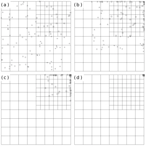
3.6 AMR bisection during refinement — 4 processes: (a) initial mesh, (b) select
new refined cells, (c) refine the mesh, (d) new domain partition (LIMA, 2012). 34
3.7 MPI Sum operation upon arrays from 4 processes — process 0 is the root.
(KENDALL, 2013). . . 36
3.8 (a) Stacks initialize with Maximum ID. (b) Stacks assign two IDs to added
particles (dashed line). . . 37
3.9 ID controller. (a) Before and (b) after particle transfer. . . 38
3.10 (a) Two dimensions block-structured mesh. (b) Lagrangian map structure —
the black discs represent the visible cells (leaves). . . 38
3.11 First case — from first to forth processes, particles are illustrated by circles,
triangles, crosses and squares, respectively. The longitudinal-section of the
3.12 Second case — from first to forth processes, particles are illustrated by circles,
triangles, crosses and squares, respectively. The longitudinal-section of the
mesh shows all particles in the aligned cells. . . 40
3.13 3D view of particles uniformly distributed in domain (first case). From first
to forth processes, particles are illustrated by circles, triangles, crosses and
squares, respectively. . . 41
3.14 3D view of particles uniformly distributed in domain (second case). From
first to forth processes, particles are illustrated by circles, triangles, crosses
and squares, respectively. . . 41
3.15 Five time steps in forced transport of particles (first case) — domain
longitu-dinal cross-section. . . 42
3.16 Four time steps in forced transport of particles (second case) — domain
lon-gitudinal cross-section. . . 43
3.17 Interpolation scheme. Solid lines represent the cell edges; dashed lines stand
for the distances D from each cell node to particle P (VEDOVOTO, 2011). . 43
3.18 Parallel, lid-driven cavity simulation — initial condition. The host processes
define particles color: blue, purple, green and red. . . 44
3.19 Longitudinal cross-section of vorticity field at z = 0.5. Particles in parallel,
lid-driven cavity simulation. . . 45
3.20 Longitudinal cross-section of the parallel, lid-driven cavity simulation on AMR. 46
4.1 Flowchart of the Lagrangian composition FDF code. . . 51
4.2 Artificial variance reduction during annihilation. . . 54
4.3 Industrial chemical reactor (left), and chemical reactor cross-section showing
some of its components (right). . . 55
4.5 Particle tracking during the first second of PaSR simulation. . . 57
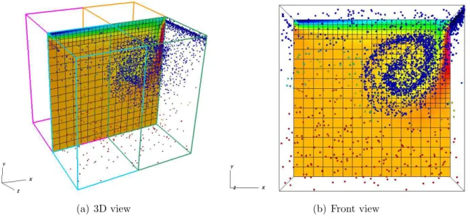
4.6 3D view of PaSR with particles colored by composition. The blue and red
colors represent the composition limits 0 and 1, respectively; the green color
stands for the global mean. . . 58
4.7 Empirical composition PDF during PaSR simulation. . . 58
4.8 Composition variance during PaSR simulation. . . 59
4.9 Multilevel, fixed mesh used on parallel, lid-driven cavity simulation.
Longitu-dinal cross-section at z = 0.5m — ∆0 = 1/32 and ∆1 = 1/64. . . . 60
4.10 Profiles of temporal composition average — PDE and SDE simulations at
t = 30.0s and Re= 500 on uniform mesh with 323 cells . N P C ranges from
60 to 360. . . 61
4.11 Profiles of temporal composition average — PDE and SDE simulations at
t = 30.0s and Re= 500 on uniform and multilevel, fixed meshes. . . 62
4.12 Comparison between PDE and SDE temporal composition average fields at
t = 30.0s, Re= 500 and z = 0.5m. . . 62
4.13 (a) Longitudinal cross-section of x−velocity field at t = 6.0s, Re= 50 and
z = 0.5m, and (b) profiles of PDE and SDE solutions at x= 0.5m. . . 64
4.14 Longitudinal cross-section of AMR — SDE cases at Re= 50 and z = 0.5m. 65
4.15 Longitudinal cross-section of temporal composition averagehζi—SDE−O60
simulation at Re= 50 and z = 0.5m. . . 65
4.16 Profiles of temporal composition average at t= 6.0s and Re= 50. . . 66
4.17 Longitudinal cross-section of variance S2 calculated based on temporal
com-position average — SDE−O60 simulation at Re= 50 and z = 0.5m. . . 67
4.18 Profiles of composition variance calculated based on temporal composition
4.19 Relationship between composition variance and vorticity at t = 6.0s and
Re = 50. (a) Isosurface |z−vorticity| = 0.5s−1
— clockwise/negative
(or-ange) and counterclockwise/positive (green). (b) Longitudinal cross-section
of |z−vorticity| and 3D view of composition variance S2 = 3·10−4
(kg/kg)2. 68
4.20 Longitudinal cross-section of notional particle density (N P C/m3) —SDE−
O60 simulation at Re= 50 and z = 0.5m. . . 69
4.21 Longitudinal cross-section of AMR — SGS cases atRe= 5000 and z = 0.5m. 69
4.22 Integral to Kolmogorov turbulence length scales,Re= 5000. . . 70
4.23 Longitudinal cross-section of effective dynamic viscosity µ+µSGS — SGS
simulation at t= 24.0s, Re= 5000 andz = 0.5m. . . 70
4.24 Profiles of effective dynamic viscosity at 24.0s and Re= 5000. . . 70
4.25 Longitudinal cross-section of temporal composition average hζi— SGS
simu-lation at Re= 5000 and z = 0.5m. . . 71
4.26 Profiles of temporal composition average at t= 6.0s and Re= 5000. . . 71
4.27 Profiles of temporal composition average at t= 24.0s and Re= 5000. . . 72
4.28 Longitudinal cross-section of variance S2 calculated based on temporal
com-position average — SGS simulation at Re= 5000 andz = 0.5m. . . 72
4.29 Profiles of composition variance calculated based on temporal composition
average at t= 6.0s and Re= 5000. . . 73
4.30 Profiles of composition variance calculated based on temporal composition
average at t= 24.0s and Re= 5000. . . 73
4.31 Relationship between composition variance and vorticity at t = 24.0s and
Re= 5000. (a) Isosurface|z−vorticity|= 0.5s−1
— clockwise/negative
(or-ange) and counterclockwise/positive (green). (b) Longitudinal cross-section
|z−vorticity|and 3D view of composition variance S2 = 2·10−2
4.1 Lid-driven cavity simulations on fixed, block-structured mesh. . . 61
Abbreviations
AM R - Adaptive, block-structured mesh
CF D - Computational Fluid Dynamics
DN S - Direct Numerical Simulation
F DM - Finite Differences method
F DF - Filtered Density Function
IEM - Interaction by Exchange with the Mean micromixing model
LES - Large Eddy Simulation
M C - Monte Carlo method
M P I - Message Passing interface
N P C - Number of Particles per Cell
P aSR - Partially Stirred Reactor
P DE - Partial Differential Equations
P DF - Probability Density Function
RAS - Reynolds Averaged Simulation
SDE - Stochastic Differential Equations
Greek
α - chemical species
δ - Dirac delta
δij - Kronecker delta
δm - initial mixture width
∆ - LES filter width
∆l - mesh length at AMR levell
Γ - molecular diffusivity
Γα - molecular diffusivity of the chemical speciesα
ΓSGS - subgrid scale molecular diffusivity
µ - dynamic viscosity
µSGS - subgrid scale viscosity
ν - kinematic viscosity
O (n) - big-Oh notation - upper bound of order n
ρ - density
hρi∆ - filtered density
τij - viscous stress tensor
τSGS
ij - subgrid scale viscous stress tensor
hτiji∆ - filtered viscous stress tensor
φ - random variable - composition
φ∗
- particle composition
φ∗
- mean particle composition
φα - composition of chemical speciesα
hφαi∆ - filtered composition of chemical species α
Φ - composition array
ψα - sample space of composition of chemical species α
Ψ - sample space of composition array Ωm - LES turbulent frequency
Ω (n) - big-Omega notation - lower bound of order n ξi - random variable with Gaussian distribution
ζ - composition field
Latin
Cs - Smagorinsky constant
CΩ - mechanical-to-scalar time-scale ratio
dW - increment of the Wiener process
fφ - filtered density function of φ
Fφ - distribution function of φ
f∆,Φ - filtered density function of the composition array Φ
f∆,uiΦ - joint velocity-composition filtered density function
G - spatial filter function
hm - initial mixture height
Jαj - molecular diffusion flux of the α chemical species in thej direction
hJαji∆ - filtered molecular diffusion flux
JαjSGS - subgrid scale molecular diffusion flux
lI - integral length scale
lk - Kolmogorov length scale
Le - Lewis number
NS - number of chemical species
p - pressure
hpi∆ - filtered pressure
Q - generic function of a physical quantity
Q′
- generic function fluctuation hQi∆ - filtered generic function
Re - Reynolds number
S2 - composition variance based on temporal composition average
Su
i - body forces in momentum transport equation
ˆ
Su
i - filtered body forces
Sα - chemical reaction rate of the α chemical species
ˆ
Sα - filtered chemical reaction
Sc - Schmidt number
ScSGS - subgrid Schmidt number
t - time
ui(xi, t) - velocity components
ˆ
ui - filtered velocity - momentum transport notation
huii∆ - filtered velocity - FDF transport notation
V - volume of a grid cell
w∗
- particle weight
Xi - spatial coordinates
Yα - mass fractions of the chemical species α
ˆ
1 INTRODUCTION 1
1.1 PDF methodology . . . 3
1.2 Monte Carlo technique . . . 3
1.3 Mixing flows . . . 4
1.3.1 Phenomenology . . . 6
2 MATHEMATICAL MODELING 13 2.1 Transport equations . . . 13
2.2 Large Eddy Simulation . . . 15
2.3 Filtered Density Function . . . 18
2.3.1 Joint velocity-composition FDF . . . 19
2.3.2 Composition FDF . . . 22
2.4 Stochastic Differential Equations . . . 24
3 LAGRANGIAN MAP 27 3.1 Adaptive, block-structured mesh . . . 27
3.2 Eulerian / Lagrangian link . . . 28
3.2.2 Search algorithm . . . 31
3.2.3 Asymptotic Algorithm Analysis . . . 32
3.3 Lagrangian distributed processing . . . 33
3.3.1 Message Passing Interface . . . 35
3.3.2 ID controller . . . 36
3.3.3 Particles initialization . . . 38
3.3.4 Forced transport of particles . . . 40
3.3.5 Particles advection . . . 42
4 LAGRANGIAN COMPOSITION FDF CODE 47
4.1 AMR3D code . . . 47
4.1.1 Temporal and spatial discretization . . . 48
4.1.2 Pressure-velocity coupling . . . 49
4.2 Lagrangian Monte Carlo algorithm . . . 50
4.3 Population of particles constraint . . . 51
4.3.1 Cloning . . . 52
4.3.2 Annihilation . . . 53
4.4 Partially Stirred Reactor . . . 54
4.4.1 Chemical reactors . . . 55
4.4.2 Mathematical models . . . 55
4.4.3 PaSR simulation . . . 56
4.5 Statistical equivalence between Eulerian and Lagrangian approaches . . . 59
4.5.1 Fixed mesh simulations . . . 60
5 CONCLUDING REMARKS 75
INTRODUCTION
Multi-species mixing flows are everywhere: in a cup of tea, individual species mix
with water until becoming a homogeneous fluid; in a car exhaust system and in an industry
chimney, the hot combustion products outflow to atmosphere and mix with pure air; and in
many industrial processes, fluids with different essences mix each other to create a specific
product.
In order to simulate this kind of flows, we present a hybrid Large Eddy Simulation
(LES) / Lagrangian composition Filtered Density Function (FDF) method on adaptive,
block-structured mesh (AMR). The LES approach solves the large scales of the flow, while
it models the small ones; on the other hand, the FDF method provides the chemical species
composition fields using the Monte Carlo method, which solves a system of stochastic
equa-tions. Moreover, the AMR is both used to numerically solve the filtered transport equations
and to represent the composition FDF using notional particles; this feature matches both
LES and Monte Carlo method good practices i.e., to increase accuracy in regions of flow
with more turbulent intensity and with sharp variations in composition field, respectively.
We focused on laminar and turbulent, non-reactive, two-species mixing flows with unit
density and constant fluid properties. However, the described mathematical and numerical
models are not restricted to those simplifications and may be used to solve a wide range of
flows, such as reactive ones. In fact, that hybrid method has great advantage when applied
of species transport equations.
To that extent, this master thesis aims at exposing the development of the parallel
Lagrangian composition FDF code and its merging with the in-house built AMR3D code.
The FDF code performs algebraic calculations over an ensemble of notional particles using
the Monte Carlo method and produces composition fields statistically equivalent to those
obtained by Finite Differences numerical solution of partially differential equations (PDE).
The complete Computational Fluid Dynamics (CFD) code allowed us to implement the
before mentioned hybrid method and to simulate mixing flows.
The first step towards this objective consisted of building a computational model of
notional particles on distributed processing environment. We achieved it constructing a
parallel Lagrangian map, which can hold different types of Lagrangian elements, including
notional particles. The map connects Lagrangian information with the Eulerian framework
of the AMR3D code, in which transport equations are solved. We used Message Passing
Interface (MPI) to communicate both Eulerian and Lagrangian data among processes.
The developed Lagrangian framework uses the multi-level hash table based onUthash.
It is built according to the Eulerian mesh. Uthash is a C header file which provides tools to
create and manipulate hash tables, and is useful to quickly manage data.
We expose an overview of mixing phenomenology on free-shear layer flow, since it is
a common studied flow, though we simulated non-compressible, lid-driven cavity, initially
segregated mixing flows to verify the statistical equivalence between Eulerian and Lagrangian
approaches for solving a composition field.
Moreover, we adopted the Schmidt number for all simulationsSc = 0.7; the Reynolds
numbers Re= 50, 500 and 5000; the fluid density ρ= 1.0; the Lewis numberLe= 1.0; and
the mechanical-to-scalar time-scale ratio CΩ = 2.0.
1.1 PDF methodology
Lagrangian Probability Density Function (PDF) methods originated in the eighties
from the junction of Eulerian PDF methods and stochastic Lagrangian models. They consist
in a feasible way to calculate the statistics of inhomogeneous turbulent flows (POPE, 1994).
An ensemble of notional particles represents a real statistical sample, wherein each
notional particle stands for a single realization of the flow in space and time. The Lagrangian
element has its own position, velocity and composition, that advance in time according to a
system of stochastic differential equations (POPE, 1994). In the composition PDF method,
the velocity comes from the Eulerian mesh by interpolation.
Peyman Givi suggested the FDF method in 1989 and Stephen Pope formulated it
one year later to numerically solve turbulent reacting flows under Large Eddy Simulation
approach (HAWORTH, 2010). Essentially, the FDF method is analogue to the PDF one in
Reynolds-Averaged Simulations. It uses the probability density function of the subgrid scale
scalar quantity to compute the effects of unresolved scalar fluctuations (COLUCCI et al.,
1998).
1.2 Monte Carlo technique
The Lagrangian FDF method uses the Monte Carlo (MC) technique to solve a derived
system of stochastic differential equations (COLUCCI et al., 1998). It works with ensembles
of notional particles, which are statistical sampling of the expected field.
Stanislaw Ulam and John von Neumann create the MC method in the forties. But it
was Nicolas Metropolis who named it, referring a story involving a famous casino in Monte
Carlo. Additionally, Enrico Fermi — a physicist who helped to create modern physics —
developed simultaneous and independently this statistical sampling technique. Figure (1.1)
shows the analogical device created by Fermi — named FERMIAC — to study neutron
transport via random choices of parameters.
Contemporary to the first electronic computer (ENIAC) and the first atomic bomb
detonation test at Alamogordo, the Monte Carlo technique is still a powerful method that
Figure 1.1: The FERMIAC device, http://en.wikipedia.org/wiki/FERMIAC, accessed on
18/04/2014.
to create MC method, since manual statistical calculations were no longer used because of
tediousness.
Many problems are unfeasible when treated by Finite Differences methods — due to
local-high gradient, for example. Instead, these are easily handled using MC. Indeed, this
algorithm is recommended to evaluate complex and multiple-dimensional integrals. Its first
scientific application was to solve the problem of neutron diffusion in fissionable materials,
wherein von Neumann had increasingly become involved (METROPOLIS, 1987).
1.3 Mixing flows
We can classify a flow based on its physical aspects and patterns of turbulence
transi-tion. It may be a free shear flow, when it occurs without geometric restrictions e.g., a wake,
a jet and a mixing layer; a boundary layer, when the flow interacts with a solid surface,
forming an intense shear region; and an enclosed flow, with strong shear effects due to the
presence of many walls (SILVEIRA-NETO, 2002).
Free-shear layer flows have a typical laminar-turbulence transition, starting with the
Kelvin-Helmholtz instabilities. They are usually found in diffusive combustion phenomena
due to the presence of two streams with different velocities, which in diffusive combustion
also present two segregate fluids, e.g., jet fire in a pipeline leakage. One can find enclosed
flows into chemical reactors and inside pipelines, for example. A mix of these two kinds of
flows occurs inside a furnace; it is composed by a jet fire that outflows to a chamber, where
hot gases circulate.
specially in turbulent regime. Among their effects, it may be cited the change in
com-pound concentrations in rivers (BOUCHEZ et al., 2010), the combustion efficiency in engines
(SOUZA; OLIVEIRA, 2010) and the losses of millions per year associated to insufficient
mix-ing in chemical reactors (PAUL; ATIEMO-OBERG; KRESTA, 2004). Figure (1.2) shows a
numerical simulation of burning gases that outflow a swirled combustor.
Figure 1.2: Instantaneous temperature field — isosurface of 1100 K. Large Eddy Simulation
of a swirled combustor during turbulent combustion (POINSOT; VEYNANTE, 2005).
Despite the origin of turbulence study is contemporary to Osborn Reynolds, with his
experiment of 1883, scientific knowledge on mixing was established in the second half of the
20th century — highlighting the publication by Nagata in 1975. Henceforth, the
understand-ing of mixunderstand-ing phenomena has allowed many engineerunderstand-ing projects (PAUL; ATIEMO-OBERG;
KRESTA, 2004).
As example of a turbulent mixing flow in nature, the work of Bouchez et al. (2010)
covers the sodium distribution in Solim˜oes river — downstream its junction with Pur´us river.
Its objective was to verify the water perfect mixture hypothesis Fig. (1.3).
Mixing is present in many industrial applications. It can be defined as the reduction of
composition, phases and/or temperature heterogeneity, aiming to achieve a desired product.
Among the industries which large losses because of mixing inefficiency in the eighties and
nineties are the chemical and pharmaceutical industries. They lost up to 10 billions per year
Figure 1.3: Aerial view of the junction of Pur´us and Solim˜oes rivers; aerial view of the
course of Solim˜oes river from its junction with Pur´us river to Manacapuru metering site; and
transversal section of Solim˜oes river showing depth profile and compounds concentration
field (BOUCHEZ et al., 2010).
1.3.1 Phenomenology
Turbulent mixing on shear flows has been subject of scientific research since the 19th
century. The work of Konrad (1977) in the seventies is one among many that have been
developed in the 20th century. During the eighties, theories experienced a breakthrough
(BREIDENTHAL, 1981; BROADWELL; BREIDENTHAL, 1982; KOOCHESFAHANI;
DI-MOTAKIS, 1986). In the nineties, an increase of the capacity and accuracy of experimental
techniques enabled a deep view into the fine-scale structures of the scalar field (BUCH;
DAHM, 1996, 1998).
The early questions that arose in the research of multiple-species, turbulent shear layer
flows were regarding the molecular mixing effect and the influence of the Reynolds number
response of 100kHz and spatial resolution of 0.1mm to study the mixture extent in these
flows. The experiment had two parallel streams of high speed helium and low speed nitrogen.
The author also analyzed streams with equal density fluids. The results revealed strong
Reynolds number influence on mixing, which increased up to 25 % with the increase in
Reynolds number.
Because species diffusion is the last step during mixing, several authors became
inter-ested in discovering the influence of the Schmidt number (Sc) on multiple-species, turbulent
shear layer flows, such as Breidenthal (1981).
The Schmidt numberSc=ν/Γ is a dimensionless parameter that expresses the relative
magnitude between the momentum ν = µ/ρ and species Γ diffusivities in a fluid. Liquids
and gases usually have Sc ≫ 1 and Sc ≈ 1, respectively. Since diffusion works towards
homogenizing the momentum and the composition fields, the smallest composition structure
— named Batchelor scale — may be even smaller than the momentum structure — named
Kolmogorov scale — in a liquid turbulent flow (FOX, 2003).
(a) side view
(b) top view
Figure 1.4: Reacting, turbulent shear layer flow. The product of reaction is dark-grey
colored (here in gray color scales); it locates around the large structures of the flow
(BREI-DENTHAL, 1981).
reactants (Sc = 600) to measure the extent of molecular mixing. Figure (1.4) shows the
visible product of reaction.
(a) (b) (c)
Figure 1.5: Concentration field — red: low-speed, black: high-speed, and the remaining
colors: mixed fluid (KOOCHESFAHANI; DIMOTAKIS, 1986).
Broadwell and Breidenthal (1982) observed two remaining unmixed streams in coherent
flow structures and proposed a model for mixing on multiple-species, turbulent shear layer
flows.
Koochesfahani and Dimotakis (1986) presented an experiment of mixing in turbulent
shear layer flows with large Schmidt number. The study covered two cases: reacting flows,
to directly measure mixing extent, and non-reacting flows, to calculate the PDF of a passive
scalar.
(a) Below mixture transition (b) Above mixture transition
Figure 1.6: PDF of composition field. The local thickness δ in the y/δ axis corresponds to
1% of the total mixed-fluid probability (KOOCHESFAHANI; DIMOTAKIS, 1986).
by fluid from high-speed stream. In the range of mixture transition, which starts
approxi-mately atRe= 5600, mixture occurs spatially and also in terms of composition change. The
maximum and minimum fluid composition varies slightly during the transversal extent of
the turbulent shear layer forRe≥5600. For flows above mixture transition, the probability
of finding an unmixed fluid in the center of the layer is 0.45. Furthermore, the mean
concen-tration is approximately constant throughout the layer (KOOCHESFAHANI; DIMOTAKIS,
1986).
(a)
(b)
Figure 1.7: (a) Scalar and (b) scalar dissipation rate fields forSc ≈1 (BUCH; DAHM, 1998).
Koochesfahani and Dimotakis (1986) proved the Schmidt number has great influence
over mixing. At high local Reynolds numbers, the normalized amount of chemical product
formed in liquid is 50 % less than in gas flows. Since molecular diffusion occurs at Batchelor
scale and liquid flows spend more time to achieve these scales than gas flows, reaction occurs
at lower rate in liquid than in gas flows.
Koochesfahani and Dimotakis (1986) produced the spatial-time picture Fig. (1.5) by
successive scans that mapped the transverse coordinate of the shear layer with spatial and
is the result of few interface regions between two streams. A green color represents the
predominant concentration of mixed fluid.
(a) (b)
Figure 1.8: (a) Scalar and (b) scalar dissipation rate fields for Sc ≈2000 (BUCH; DAHM,
1996).
Figure (1.6) shows two delta functions atζ = 0 andζ = 1, revealing the predominance
of unmixed fluid in shear layer. The rich high speed fluid (ζ = 1) in the cores of vortex
structures is highlighted in y/δ axis. Figure (1.6) also shows the fluid composition changes
towards the mean concentration (ζ = 0.6), shaping a new delta function.
The multiple-species, turbulent shear flows present a similar fine-scale structure of
scalar dissipation rate field at high and nearly unit Schmidt number. This structure is formed
by strained, laminar and sheet-like diffusion layers (BUCH; DAHM, 1998). Buch and Dahm
(1996, 1998) investigated the composition field in turbulent shear flows at Sc ≈ 2000 and
Sc≈1. The resolution and signal quality of measurements led to obtain the scalar and the
instantaneous dissipation rate of scalar energy fields.
Figures (1.7) and (1.8) show the scalar and the scalar dissipation rate fields for gas and
liquid flows, respectively. They highlight the fine-scale similarity between these two flows,
and reveal liquid flows have scalar wave-lengths smaller than gas flows.
We have exposed an overview of mixing phenomenology on free-shear layer mixing
flows from large to small turbulence scales. It grants us understanding on the physics of the
flow and support us to apply mathematical models that agree with these physics e.g., LES
In this way, the experiments presented in this section were neither simulated nor had
their results compared against numerical data; instead, our simulations covered just enclosed,
mixing flows. Even though, the general relation between Reynolds number and mixing extent
described in this section could be observed on our results.
The next chapter shows the mathematical modeling for the multiple-species mixing
flows we have described. Section 2.1 presents the transport equations of mass, momentum
and chemical species’ mass fraction with the closures for the viscous stress tensor and the
molecular diffusion flux. Section 2.2 covers the Large Eddy Simulation approach which
separates turbulent flow scales in order to numerically solve the large scales and model
the small ones. We show the filtered density function concept and the composition FDF
transport equation in section 2.3. The derived system of stochastic differential equations for
composition transport appears in section 2.4.
Chapter 3 shows the Lagrangian map and the overall computational framework
devel-oped to support the Lagrangian composition FDF code. It also present results concerning
particles transport in parallel environment. Section 3.1 explains what is an adaptive,
block-structured mesh to which the Lagrangian map must conform. Section 3.2 shows how the link
between the Eulerian and Lagrangian frameworks was achieved. We cover the Lagrangian
distributed processing in section 3.3, showing some of the Message Passing Interface terms
and functions, as well as the particle identifiers controller.
Chapter 4 exposes the developed Lagrangian composition FDF code, which
communi-cates with the Finite Differences framework of the AMR3D code. Section 4.2 describes the
Lagrangian Monte Carlo algorithm that is applied upon the system of stochastic differential
equations to solve the composition field of the flow. Section 4.3 covers the central point of
MC solver: the population of notional particles constraint. We present the Partially Stirred
Reactor concept, some mathematical models and a single box PaSR simulation in section 4.4.
The statistical equivalence between Eulerian and Lagrangian approaches appears in section
4.5; this section also presents simulations of enclosed, initially segregated multiple-species
MATHEMATICAL MODELING
This chapter describes the hybrid Large Eddy Simulation (LES) / Lagrangian Filtered
Density Function (FDF) mathematical model implemented in the AMR3D code (VILLAR,
2007; LIMA, 2012). Section 2.1 details the transport equations of mass (continuity),
mo-mentum (Navier-Stokes) and composition; section 2.2 describes the LES approach used to
filter these equations, as well as the closure models required for numerical solutions; sections
2.3 and 2.4 refer to the FDF transport equations and to the system of derived stochastic
differential equations (SDE).
2.1 Transport equations
The transport equations for reactive flows, with velocity vector ui(xi, t) (i = 1,2,3),
density ρ(xi, t) and chemical species mass fraction array Yα(xi, t) (α = 1,2, ..., N s) is
spa-tially,xi, and temporally, t, dependent
∂ρ ∂t +
∂ρui
∂xi
= 0, (2.1)
∂ρui
∂t +
∂ρuiuj
∂xj
=−∂p
∂xi
+∂τij
∂xj
+Siu, (2.2)
∂ρYα
∂t +
∂ρujYα
∂xj
=−∂Jαj
∂xj
where: τij, Siu, Sα and Jαj stand for viscous stress tensor, body forces, chemical reaction
rate and molecular diffusion flux for species α, respectively;i and j are directions in which
summation apply; pis the pressure.
For a Newtonian fluid, the viscous stress tensor is modeled as
τij =µ
Ç
∂ui
∂xj
+∂uj
∂xi å − 2 3µ ∂uk ∂xk
δij, (2.4)
where,µ is the fluid molecular viscosity andδij is the delta Kronecker tensor.
The molecular diffusion flux Jαj is modeled using Fick’s law of diffusion
Jαj =−
µ Sc
∂Yα
∂xj
, (2.5)
where: Sc =ν/Γαis the Schmidt number;νand Γαare the kinematic viscosity and molecular
diffusivity for species α, respectively. The following equations assume an equal molecular
diffusivity to all species, Γα = Γ, and a unit Lewis number, Le= 1.
When a flow comprises thermal energy exchange, it is useful to group Yα from Eq.
(2.3) and the enthalpy into a single generic scalar variable, φα. The transport equation of
that generic scalar becomes
∂ρφα
∂t +
∂ρujφα
∂xj
=−∂Jαj
∂xj
+Sα, (2.6)
with
Jαj =−ρΓ
∂φα
∂xj
. (2.7)
Vedovoto (2011) presented more details about the enthalpy transport and the generic scalar
modeling.
At this point one could numerically solve the presented N s+ 3 transport equations
Eqs. (2.1) to (2.3) with their closures Eqs. (2.4) and (2.5) — just N s−1 equations must
be solved in order to get all N s species, because N sP
of equations also increases. Additionally, all flow’s degrees of freedom must be captured by
the computational mesh on Finite Differences or Finite Volume approaches. Both scenarios
may be impracticable for high Reynolds number flows and nowadays available computational
resources.
We introduce a hybrid LES / Lagrangian FDF method which is an alternative approach
to numerically solve mixing flows, specially for reactive and combustion ones. The FDF
methodology greatest advantage is to present the chemical reaction rate term in a closed
form, free from modeling efforts needed in Finite Differences method (VEDOVOTO, 2011).
2.2 Large Eddy Simulation
We can divide the wavelengths of the flow into large (resolved) and small (modeled)
scales — captured and not captured by the computational mesh, respectively. This strategy is
called Large Eddy Simulation in computational study of turbulent flows (SILVEIRA-NETO,
2002). Direct Numerical Simulation (DNS) and Reynolds Averaged Simulation (RAS) are
alternative approaches. The former solves every scale of the flow, while the latter solves the
mean field.
In order to choose the best approach to numerically solve the mathematical model of a
given flow, a question must be answered: how much the large and the small scales affect the
flow? In a turbulent free shear flow, the large scales control the flow dynamics. Molecular
mixing occurs at the smallest scales — regarding space and time — and determines how
momentum and species concentration fields evolve (HAWORTH, 2010).
We present the spatial filtering operation over the mathematical model developed in
section 2.1. Given Q any function of a physical quantity (e.g., ui or Yα), its local spatially
filtered valuehQi∆ is defined as the integral over the flow domain
hQi∆ =hQ(xi, t)i∆≡
Z
Q(yi, t)G(|yi−xi|)dy, (2.8)
+R∞ −∞
G(zi)dz = 1 for zi =|yi−xi|,
G(zi) =
1/∆3 if zi ≤∆, i= 1,2,3
0 otherwise
, (2.9)
where, ∆ =V1/3 and V is the cell volume.
Therefore, the instantaneous value of Q(xi, t) can be decomposed into its filtered
hQ(xi, t)i∆and fluctuation Q ′
(xi, t) parts. Two properties of filters are (SILVEIRA-NETO,
2002):
• To filter a filtered quantity affects its value
hhQi∆i∆6=hQi∆; (2.10)
• The filter of a fluctuation is not equal zero
¨
Q′∂
∆ 6= 0. (2.11)
Applying these properties on the set of equations (2.1 to 2.3) we have,
∂hρi∆
∂t +
∂hρi∆ubi
∂xi
= 0, (2.12)
∂hρi∆ubi
∂t +
∂hρi∆ubiubj
∂xj
=−∂hpi∆
∂xi
+∂hτiji∆
∂xj
+ ∂τ
SGS ij
∂xj
+S“iu, (2.13)
∂hρi∆Y“α
∂t +
∂hρi∆ubjY“α
∂xj
=−∂hJαji∆
∂xj
+∂J
SGS αj
∂xj
+S“α, (2.14)
where: hi∆andbare both filter notations equivalently used throughout this chapter;τSGS ij =
hρi∆ubiubj− hρi∆’uiuj andJαjSGS =hρi∆ubjY“α− hρi∆u’jYα are the subgrid scale (SGS) stress and
the SGS molecular diffusion flux, respectively.
Turbulent mixing analysis requires to establish models for τSGS
ij and JαjSGS in order
instantaneous variables are unknown (e.g.,’uiuj and u’jYα).
In reacting flows, Eq. (2.14) demands a model for the filtered chemical reaction term.
The FDF formulation attends this requeriment presenting this term in a closed form. It is
the main benefit of the FDF schemes (COLUCCI et al., 1998), since the filtered chemical
reaction term modeling is difficult due to the non-linear relationship between chemical
reac-tion and turbulence (FOX, 2003). Fox (2003) presents alternative approaches for modeling
the chemical reaction term for LES and RAS perspectives.
The key point for modeling whatever SGS quantity is its relationship with a known
large scale. In the case of the unknown SGS stress, the Smagorinsky eddy viscosity closure
may relate this term with the local large scale rate of flow strain (COLUCCI et al., 1998).
By applying the Smagorinsky model, Eq. (2.13) incorporates a SGS viscosity µSGS in
the filtered stress term. The modeled filtered stress is represented by
hτijiM∆ =
Ä
µ+µSGSä ñÇ∂ubi ∂xj
+ ∂ubj
∂xi
å
− 2 3
∂ubk
∂xk
δij
ô
, (2.15)
where the SGS viscosity — also called apparent or turbulent viscosity — is proportional to
the filtered strain rateS“ij,
µSGS = (Cs∆)2hρi∆S“, (2.16)
S“=Ä2S“ijS“ij
ä1/2
, (2.17)
“
Sij =
1 2
Ç
∂ubi
∂xj
+∂ubj
∂xi
å
, (2.18)
andCsis the Smagorinsky constant, which value 0.2 is used for isotropic turbulence (FERZIGER;
PERIC, 1996).
The gradient diffusion concept relates the unknown SGS molecular diffusion flux with
the known filtered species’ mass fraction (FOX, 2003) — a similar approach used by applying
Fick’s law in Eq. (2.5) —
JSGS
αj =−hρi∆ΓSGS
∂Y“α
∂xj
where,
ΓSGS = 2hρi∆(Cs∆) 2
ScSGS
S“= µ
SGS
ScSGS, (2.20)
ΓSGS is the SGS molecular diffusivity andScSGS is the SGS Schmidt number, which controls
the magnitude of turbulent molecular diffusion (VEDOVOTO, 2011).
The filtered transport equations Eqs. (2.12) to (2.14), the closure models Eqs. (2.15)
to (2.20) and a chemical kinetics mechanism are sufficient to solve reactive and low Mach
number flows.
Although the mathematical model presented in this chapter is in accordance with the
flows of interest (i.e., variable density, multi-species reactive and low Mach number flows), the
developments and the simulations presented in this master thesis are focused on two-species,
non-reactive and incompressible (unit density fluid) flows.
2.3 Filtered Density Function
The Filtered Density Function is the Probability Density Function (PDF) of SGS
variables (COLUCCI et al., 1998). Whilst the PDF length scales are restricted to the
turbulence integral scalelT, the FDF length scales fulfill a range down to the characteristic
filter width (HAWORTH, 2010).
The FDF of a random variableφ (e.g., composition) is defined as the derivative of its
distribution function with respect to its sample spaceψ (i.e., its domain)
fφ(ψ)≡
dFφ(ψ)
dψ , (2.21)
and the distribution function is defined as the probability of that variable be lesser than ϕ,
Fφ(ψ)≡P (φ < ϕ). (2.22)
Ψ defines the FDF at pointxi and time t (FOX, 2003),
f∆,Φ(Ψ;xi, t)≡P rob{(Ψ <Φ (xi, t)<Ψ +dΨ)}, (2.23)
where, Φ is the random variable array and Ψ is its sample space.
Considering Φ the array of chemical species mass fractions Yα, the composition FDF
can be expressed as the integral of the Dirac delta function δ and the spatial filter G from
Eq. (2.9),
f∆,Φ(Ψ;xi, t)≡
Z
δ(Ψ−Φ (yi, t))G(yi −xi)dy, (2.24)
where the integral covers the flow domain, and
δ[Ψ−Φ (yi, t)]≡ N s
Y
α=1
δ[ψα−φα(yi, t)]. (2.25)
Since δ[Ψ−Φ (yi, t)] is the detailed, low-level density, the composition FDF can be
understood as theG filtered density (COLUCCI et al., 1998).
We present two ways for deriving the composition FDF transport equation. The first
starts from the transport equations (2.2) and (2.3) and further integrates the joint
velocity-composition FDF on velocity space in order to generate the velocity-composition FDF (section 2.3.1);
the second starts from the time derivative of Eq. (2.24) (section 2.3.2).
2.3.1 Joint velocity-composition FDF
The joint velocity-composition FDF transport equations are an alternative
mathemat-ical model for the physmathemat-ical system being treated in this master thesis. This model considers
both the momentum and composition fields in a probabilistic manner.
The probability of the random velocity vectorui and the random species mass fraction
velocity-composition FDF at point xi and time t (FOX, 2003)
f∆,uiΦ(vi,Ψ;xi, t) ≡ P rob{(vi < ui(xi, t)< vi+dvi)} ∩
P rob{(Ψ <Φ (xi, t)<Ψ +dΨ)}. (2.26)
The joint FDF is valuable because we can use it to derive all one-point statistics ofui
and Φ, for example the filtered velocityubi, the filtered compositionφbα, the Reynolds stresses
’
uiuj, the composition fluxes ubiφ ′
α and the filtered chemical reaction rate S“α. However,
transported FDF methods need closures for two-point dependent terms; therefore, pressure
fluctuation gradient, viscous and species diffusion need additional modeling (FOX, 2003).
In order to derive the joint FDF transport equation from Eqs. (2.2) and (2.3), two
independent expressions for the filtered total derivative of an arbitrary, one-point scalar
function of velocity and composition Q(ui,Φ) must be found and further equated (FOX,
2003).
The filtered value of Q(ui,Φ) is related with the joint FDF by
hQ(ui,Φ)i∆=
Z Z
Q(vi,Ψ)f∆,uiΦ(vi,Ψ;xi, t)dvdΨ, (2.27)
where the integrals cover all vi and Ψ domains.
Firstly, we rewrite the transport equations in a compact and simplified form
Dui
Dt ≡ ∂ui
∂t + ∂uiuj
∂xj
=Ai, (2.28)
Dφα
Dt ≡ ∂φα
∂t + ∂ujφα
∂xj
= Θα, (2.29)
where,
Ai ≡ −
∂p ∂xi
+∂τij
∂xj
+Siu, (2.30)
Θα ≡
∂Jαj
∂xj
+Sα. (2.31)
Q(ui,Φ) can be expressed as Æ DQ Dt ∏ ∆
= ∂hQi∆
∂t +
∂hujQi∆
∂xj
. (2.32)
Combining Eq. (2.32) with Eq. (2.27), and sincevi and Ψ are integration variables, it
becomes Æ DQ Dt ∏ ∆ = Z Z
Q(vi,Ψ)
®
∂f∆,uiΦ
∂t +vj
∂f∆,uiΦ
∂xj
´
dvdΨ. (2.33)
The chain rule is the starting point to derive the second form of the filtered total
derivative of Q(ui,Φ),
DQ Dt = ∂Q ∂uj Dui Dt + ∂Q ∂φα Dφα
Dt . (2.34)
Furthermore, substituting Eqs. (2.28) and (2.29) into Eq. (2.34) and applying the
filter, we have
Æ DQ Dt ∏ ∆ = Æ ∂Q ∂uj Ai ∏ ∆ + Æ ∂Q ∂φα Θα ∏ ∆ , (2.35)
in which the conditional filter — see Fox (2003) — is considered to give
Æ DQ Dt ∏ ∆ =− Z Z
Q(vi,Ψ)
®
∂ ∂vj
[hAi|vi,Ψif∆,uiΦ] +
∂ ∂ψα
[hΘα|vi,Ψif∆,uiΦ]
´
dvdΨ. (2.36)
Finally, the final form of the joint FDF transport equation is achieved by subtracting
Eq. (2.36) from Eq. (2.33)
∂f∆,uiΦ
∂t +
∂ujf∆,uiΦ
∂xj
=− ∂
∂vj
[hAi|vi,Ψi∆f∆,uiφ]−
∂ ∂ψα
[hΘα|vi,Ψi∆f∆,uiΦ]. (2.37)
Since the joint velocity-composition FDF transport equation has random variables
describing three velocity componentsui and the array of chemical species Φ, when we
inte-grate Eq. (2.37) over the velocity sample spacevi, it results the composition FDF transport
Because this integration eliminates the velocity field, it is necessary to provide the
momentum information and to treat the turbulence through a different model. Therefore,
the composition and velocity fluctuations link no longer exists, and a FDF composition
flux model is consequently required. For both joint FDF and composition FDF models, a
micromixing model is necessary to calculate the molecular diffusion response on both FDF
shape and rate of composition variance decay (FOX, 2003).
As mentioned before, we present in section 2.3.2 a second form for deriving the
compo-sition FDF transport equation. It starts from the compocompo-sition FDF definition as the integral
of the Dirac delta function δ and the spatial filter G from Eq. (2.9).
2.3.2 Composition FDF
The time derivative of Eq. (2.24) is
∂f∆,Φ(Ψ;xi, t)
∂t = −
Z ∂φ
α(yi, t)
∂t
∂δ[Ψ−Φ (yi, t)]
∂ψα
×G(yi−xi)dy
= − ∂
∂ψα
Z ∂φ
α(yi, t)
∂t ×δ[Ψ−Φ (yi, t)]G(yi−xi)dy. (2.38)
Considering the conditional filter of Q(xi, t), which is any function of Yα,
hQ(xi, t)|Ψi∆≡
R
Q(yi, t)δ[Ψ−Φ (xi, t)]G(yi−xi)dy
f∆,Φ(Ψ;xi, t)
. (2.39)
When Q(xi, t) is the partial, time derivative of φα(xi, t), Eq. (2.38) becomes
∂f∆,Φ(Ψ;xi, t)
∂t =−
∂ ∂ψα "Æ ∂φα ∂t Ψ ∏ ∆
f∆,Φ(Ψ;xi, t)
#
. (2.40)
For a unit density flow, Eq. (2.3) can be simplified. Substituting the reduced form of
Eq. (2.3) in Eq. (2.40), we have
∂f∆,Φ(Ψ;xi, t)
∂t =
∂ ∂ψα
"Æ
∂ujφα
∂xj Ψ ∏ ∆
f∆,Φ(Ψ;xi, t)
# + ∂ ∂ψα "Æ ∂Jαj ∂xj Ψ ∏ ∆
f∆,Φ(Ψ;xi, t)
#
(2.41)
− ∂
∂ψα
The whole transport equation ofφα is conditioned to its sample space Ψ inside the
compo-sition FDF transport equation.
The first right hand side of Eq. (2.41) is the unclosed convective term. We can change
the ψα derivative by the spatial one (COLUCCI et al., 1998)
−∂huj |Ψi∆f∆,Φ(Ψ;xi, t)
∂xj
. (2.42)
A similar procedure used in LES,
hujφαi∆ =huji∆hφαi∆+
î
hujφαi∆− huji∆hφαi∆
ó
, (2.43)
is applied to divide large from subgrid scales Eq. (2.44). In fact, Eq. (2.43) is the first
moment of
huj |Ψi∆f∆,Φ =huji∆f∆,Φ+
î
huj |Ψi∆− huji∆
ó
f∆,Φ, (2.44)
which gives us a closed term, which represents the filtered convection of f∆,Φ in Cartesian
space, and an unclosed term called subgrid convective flux, which represents the effects of
unresolved SGS convection. Large eddy simulation must provide huji∆ (COLUCCI et al.,
1998).
Finally, the filtered density function f∆,Φ transport equation becomes
∂f∆,Φ
∂t +
∂huji∆f∆,Φ
∂xj
= −∂
î
huj |Ψi∆− huji∆
ó
f∆,Φ
∂xj + ∂ ∂ψα "Æ ∂Jαj ∂xj Ψ ∏ ∆
f∆,Φ #
− ∂[Sα(Φ)f∆,Φ]
∂ψα
, (2.45)
whose unclosed terms we must model. These terms are the SGS convective flux — mentioned
above — and the diffusion term, which expresses the influence of molecular diffusion on FDF
transport. The last right hand side term is a closed form of the chemical reaction rate.
The SGS convective flux is modeled as
î
huj |Ψi∆− huji∆
ó
f∆,Φ =−ΓSGS
∂f∆,Φ
∂xj
whose first moment is given by Eq. (2.19).
We may divide the diffusion term into two parts
− ∂ ∂ψα "Æ ∂Jαj ∂xj Ψ ∏ ∆
f∆,Φ #
= ∂
∂xj
Ç
Γ∂f∆,Φ
∂xj
å
− ∂
2
∂ψα∂ψβ
"Æ
Γ∂φα
∂xj ∂φβ ∂xj Ψ ∏ ∆
f∆,Φ #
. (2.47)
The first right hand side term of Eq. (2.47) represents the effects of molecular diffusion in
spatial transport of FDF, while the second — called conditional SGS diffusion — represents
the dissipative nature of subgrid scalar mixing. We can model the conditional SGS diffusion
using, for instance, the Interaction by Exchange with the Mean (IEM) closure (COLUCCI
et al., 1998)
− ∂
∂ψα
[Ωm(ψα− hφαi)f∆,Φ], (2.48)
where Ωm is the subgrid frequency of mixing. This frequency depends on large scale variables;
in LES, we can relate it with the SGS diffusion coefficient, the filter width and an assumed
constant mechanical-to-scalar time-scale ratio CΩ (VEDOVOTO, 2011),
Ωm =CΩ
Ä
Γ + ΓSGSä¿∆2. (2.49)
The final form of the composition FDF transport equation is
∂f∆,Φ
∂t +
∂huji∆f∆,Φ
∂xj
= ∂
∂xj
ÇÄ
Γ + ΓSGSä∂f∆,Φ
∂xj
å
+ ∂
∂ψα
[Ωm(ψα− hφαi∆)f∆,Φ]−
∂[Sα(Φ)f∆,Φ]
∂ψα
, (2.50)
with all closures applied.
2.4 Stochastic Differential Equations
We used a system of stochastic differential equations equivalent to Eq. (2.50), which
gives us all composition statistics. Although we can handle these equations based on Eulerian
and Lagrangian frameworks, we chose the latter approach because it is more accurate than
Both Eulerian and Lagrangian Monte Carlo use notional particles to carry the
composi-tion FDF. Those particles are transported in Cartesian space by large scales, SGS conveccomposi-tion
and molecular diffusion; particle composition changes due to SGS diffusion and chemical
re-action. However, notional particles are mesh independent in Lagrangian approach, while
they are mesh dependent in Eulerian (COLUCCI et al., 1998).
The following system of stochastic differential equations models the general diffusion
process (COLUCCI et al., 1998):
dXi(t) = Di
~
X(t), tdt+EX~ (t), tdWi(t), (2.51)
where the coefficients come from a comparison between Eq. (2.51) and Eq. (2.50)
E ≡»2 (Γ + ΓSGS), (2.52)
Di ≡ huii∆+
∂ÄΓ + ΓSGSä
∂xi
, (2.53)
which need the filtered velocity and the SGS molecular diffusivity from large eddy simulation.
The stochastic equation that describes the particles spatial evolution is
dXi(t) =
huii∆+ ∂
Ä
Γ + ΓSGSä
∂xi
dt+î2ÄΓ + ΓSGSäó1/2dW
i, (2.54)
wheredW(t) is a statistical independent increment — the Wiener noise.
The stochastic equation that describes the evolution of particles composition is
dφ∗
α
dt =−Ωm(φ
∗
α− hφαi∆) +Sα, (2.55)
where,φ∗
αis theαspecies composition of the notional particle and Ωmis the subgrid frequency
of mixing Eq. (2.49). The term that comprises this frequency is the IEM micromixing model.
It is a current subject of research which requires more development (ORBEGOSO, 2007).
One can calculate the composition first moment hφαi∆ and its higher moments (e.g.,
variance) using the particles ensemble in each Eulerian cell described in chapter 3.
preserve the Markovian character of the diffusion process (VEDOVOTO, 2011)
Xip(tn+1) =Xip(tn) +Dpi (tn) ∆t+Ep(tn) ∆t1/2ξpi (tn), (2.56)
where, n stands for the current time step, p represents the particle and ξip is a random
LAGRANGIAN MAP
This chapter aims at exposing the main features of the Lagrangian map, which we
developed during this work. It is a Lagrangian framework linked to the well established
Finite Differences framework of the in-house built AMR3D code (VILLAR, 2007; LIMA,
2012). The map consequently supports a hybrid LES / Lagrangian FDF method we have
implemented and applied.
3.1 Adaptive, block-structured mesh
The adaptive, block-structured mesh — hereafter referred by the acronym of the
Adap-tive Mesh Refinement (AMR) family methods — is a computational technique used to
dy-namically achieve high numerical precision on flow regions of interest using Finite Differences
(FD) method or analogous. It greatly contributes to minimize the required computational
resource and the simulation time because distributes cell nodes heterogeneously throughout
flow domain. Figure (3.1) shows three levels of mesh resolution, which are more refined near
the top and right edges.
The greatest disadvantage of an adaptive, block-structured mesh is its inflexibility
to fit complex domains and immersed objects. However, Lagrangian based methods like
Immersed Boundary and Front Tracking have been successfully applied to overcome that
Figure 3.1: Longitudinal cross-section of AMR in 3D domain with 3 grid levels.
domain borders and objects displacements. In both cases, the link between mesh and particle
variables occurs by interpolation.
In the AMR3D code, the flow variables (e.g., velocity and species mass fraction) evolve
on adaptive, block-structured mesh. The refinement criterion is based on the magnitude of
the vorticity field. If we set a mesh with 3 grid levels and a refinement range of 5%, the first
and second finest mesh will cover the regions of the flow within [0.95−1.0] and [0.9−0.95]
of the greatest vorticity intensity; the coarsest mesh will cover all flow domain.
That mesh is easily parallelized compared to unstructured mesh (LIMA, 2012). Lima
(2012) discoursed on AMR3D parallelization methods, and used Message Passing Interface
(MPI) to communicate Eulerian based data among processes. We used the same approach to
communicate Lagrangian information using the parallel Lagrangian map, as it will be seen
in section 3.3.
3.2 Eulerian / Lagrangian link
Many are the flows which involve Lagrangian elements, like particles for instance. The
computational particle can represent distinctive natures, for example a particulate in
gas-solid flow or a stochastic element in a reactive flow, with physical and numerical essence,
respectively. Nowadays, the majority of literature addresses Lagrangian transport on
ANTYPAS; DALEY, 2011).
The computational model of a system — preceded by the physical, the mathematical
and the numerical models — is crucial considering the quality of a Computational Fluid
Dynamics (CFD) software. The Eulerian / Lagrangian modeling requires a data structure
able to exchange information between these two frameworks. Moreover, the direct access
to the ensemble of particles contained in each cell is essential to the Lagrangian FDF code
performance, especially regarding algorithms dependent on sorting (FOX, 2003).
Two questions arise when we observe the transport of particles in Eulerian domain
— specially on AMR. First, which particles dwell in a given cell; second, which is the host
cell of a specific particle. The Lagrangian map answers both questions. It is composed by
a multi-level hash table that provides direct access to the ensemble of particles contained in
each cell Fig. (3.2), and uses a per level search tool based on algebraic equation Eq. (3.1)
to find the cell in which the particle resides.
ID
Cell
Level 1
Cell
Level 2
Multi-level Hash Table Particles Hash Table
Figure 3.2: Lagrangian map: computational model composed by a multi-level hash table of
identifiers (ID) and a particles hash table.
Figure (3.2) shows that the first hash tables are always cell-type and the last one is
hash table depends on Eulerian mesh, the code must rebuild its structure at each mesh
refinement. In a 3D domain, each coarse cell originates eight fine cells.
3.2.1 Hash table
Data structures store data into and acquire data from random-access memory and
hard disc. Many are based on predefined size arrays, which use an integer index to address
data, others are based on linked lists, which dynamically connect data using pointers; hash
tables provide a mixture of these features. Shaffer (2013) described several data structures
and their applicability.
Hash table is a dynamic data structure that allows direct reference to storage and
access data. The reference occurs by a key, which can be an integer, a character or an
user-defined type. Therefore, each data of a collection must have a unique key. The pairing rule
used to attend this request is called hash function. When we try to storage two data using
the same key, a collision occurs.
Figure (3.3) shows the AMR is an inherent collision system: the key of each cell is its
index (i, j, k), which is the same to a refined cell and the correspondent low-level coarse cell.
It occurs because these cells have the same origin.
Figure 3.3: The same key (1,1,1) used to the coarse and refined cells leads to hash table
collision.
A collision resolution policy is practiced by applying the open hashing or the closed
into the same hash table, just using another key. When it uses another hash table to save
the data, it is called open hashing (SHAFFER, 2013).
The developed Lagrangian framework applies the open hashing using the multi-level
hash table based onUthash (HANSON, 2013). Uthash is a C header file developed under the
revised BSD license in 2006 by Troy D. Hanson due to the lack of this kind of data structure
in the standard C library. Several commercial and academic software have incorporated it
since the first release. Uthash provides tools to create and manipulate hash tables (e.g.,
addition, deletion and searching), which are O(1) for time processing.
3.2.2 Search algorithm
Many computational applications foment business, help communication and model the
physical world (e.g., service, engineering and scientific software). They all need some kind
of search mechanism to operate over a database. The code can invoke them several times —
what makes these algorithms attractive in terms of efficiency improvement.
Search algorithms are classified based on the desired response. The exact-match and
therange query verify a data existence and the relative position of a data among a collection,
respectively. The search approach also varies according to the kind of information — whether
data is sorted or not, small or large, integer or floating-point, directly or indirectly accessed
(SHAFFER, 2013).
Sequential, binary and dictionary based searches apply to orderly collections of data.
The sequential search presents O(n) — n stands for the amount of data — and analyses
each value, comparing them with the sought data. It is inefficient for great collections and
frequently demanded operations. The binary search isO(log (n)) and split the investigation
in consecutively two sub domains. The dictionary based search is similar to the binary
one, though more efficient. It is O(log log (n)) because it knows how data are distributed,
optimizing the domain split (SHAFFER, 2013). Since mesh width is uniform per level in
AMR, the search tool can use a direct mechanism based on the algebraic equation
index=f
Ñ
~ P −P~0
∆l
é