Cost/Revenue Trade-Off of Small Cell Networks in the Millimetre Wavebands

Cost/Revenue Trade-off of Small Cell Networks in

the Millimetre Wavebands

Emanuel Teixeira, Fernando J. Velez

6201-001 Covilhã, Portugal [email protected] , [email protected]

Abstract: In this work, we identify and discuss the potentialities of mobile cellular communications in the millimetre wavebands, showing that very high bit/data rates can be supported in small cells with short-range coverage. We study the behaviour of the carrier-to-noise-plus-interference ratio with the coverage distance (and the actual distance from users to the eNBs) in actual environments and the respective analysis of the impact in cellular planning and optimization process. We assess the equivalent supported throughput within cells with reuse pattern K=2, assuming, in this preliminary phase, the use of LTE. In terms of cell coverage and the computation of interference, LoS propagation models have been considered at the 28, 38, 60 and 73 GHz frequency bands. From these analytical computations, we conclude that, at 28 GHz, although lower system capacity is achieved for very short coverage distances of the order of 25 m, in comparison to the 73 GHz frequency band, there is an enhancement in the supported throughput for longer coverage ranges, and it is clearly more favourable for the lowest frequency band. Owing to the additional attenuation of oxygen, the 60 GHz frequency band is more challenging, as the lowest values of the co-channel interference due to the additional oxygen attenuation originate higher values for the supported throughput, even for lower values of the reuse pattern.Based on these results, costs and revenues are studied. Revenues are proportional to the supported throughput and the profit is generally a declining function with cell radii. The highest profit corresponds to the shortest cell radii, up to 80 m, and the best results occur for the 28 GHz band.

Keywords: Millimetre Waves (mmW), 4G evolution to 5G, LTE, LoS propagation models, interference, CNIR, LTE-U.

I. INTRODUCTION

The millimetre wavebands can provide high bit rates in short range applications while being supported by much smaller antennas. However, in general, they suffer from higher path loss but may also have the advantage of additional oxygen absorption to reduce interference, e.g., in the 60 GHz frequency band, as described in [1], [2]. In real environments, cellular mobile connections are simultaneously affected by noise and co-channel interference. Moreover, in the cellular planning process, the understanding of the variation of the carrier-to-noise-plus-interference ratio (CNIR) for mobile communications are of utmost importance. To study the joint contribution of all these factors in the optimization process, this paper performs a comparison of the CNIR and the equivalent supported throughput among different frequency bands for regular shaped cellular topologies such as the Manhattan grid topologies or linear topologies, like main roads or highways, as shown in

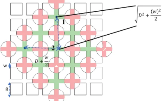
Figure 1. In fact, it is straightforward to show that, in the downlink (DL), the worst-case bounds for CNIR from a Manhattan grid topology shown in Figure 2 are like the worst-case bounds from a linear cellular topology. In order to simplify the computations, in this phase, we assume the linear topology from Figure 1, with reuse pattern two, i.e., K=2 [3].

The cell coverage and frequency reuse trade-off is analysed by considering the appropriate propagation models, in order to examine the influence of oxygen in the path loss at 60 GHz. The CNIR is studied in detail, as well as the underlying throughput in other frequency bands at the millimetre wavebands. These future systems will use 5G air interfaces that will consider, e.g., Filter Bank Modulation Carrier (FBMC). However, in the near-future LTE Unlicensed (at 3.5 and 5 GHz) is still considering OFDMA in the DL, with maximum bandwidths of 20 MHz. As a working assumption, we are considering the use of OFDMA, as in the DL of LTE Unlicensed (LTE-U), and bandwidth of 20 MHz. Hence, 100 resource blocks (RBs) are assumed. The propagation exponent is =2.1 for 28 GHz, and =2.3 for 40 GHz, 60 GHz and 73 GHz.

By considering the results for the system capacity arising from this analysis, one examines the cost/ revenue trade-off. Costs depend on the prices for the spectrum license and equipment, operation and maintenance, as well as on the number of cells and cell radius, and take advantage of unlicensed bands.

Fig. 1. Linear topology with cigar-shaped cells, with reuse pattern 2, considered in the analysis of CNIR in the millimetre wavebands.

Fig. 2. Manhattan Topology (position 1 and 2).

𝐷2₊ 𝑤 2 2 R w 𝐷 + 𝑤 2

This work has been partially supported and funded by CREaTION, COST CA 15104, ECOOP, UID/EEA/50008/ 2013 and Bolsa BID/ICI-FE/Santander Universidades-UBI/2017. D D+d D-d 1 2 d 978-1-5386-6355-4/18/$31.00 ©2018 IEEE

Revenues depend on the price per MB and on the supported throughput.

The remainder of the paper is organized as follows. Section II starts by presenting path loss models in millimetre wavebands, and then addresses the influence of interferers in the system, for the Manhattan and linear topologies. Section III presents the study of the system in terms of the CNIR and PHY Throughput. In Section IV, simulation and analysis of the results for CNIR and PHY Throughput are continued to study system Capacity. While in Section V, a cost/revenue model is studied in order to optimise the system. Finally, conclusions are drawn in Section VI.

II. CARRIER-TO-INTERFERENCE RATIO IN THE MILLIMETRE WAVEBANDS

In order to describe the behaviour related to the losses in the millimetre wavebands in Line-of-Sight (LoS), the path loss is defined by the following equation [4], [5], [6], [7]:

𝑃𝐿 𝑑𝐵 𝑑 = 20𝑙𝑜𝑔10 4𝜋𝑑0 𝜆 + 10𝑛 𝑙𝑜𝑔10 𝑑 𝑑0 + 𝑋𝜎, 𝑑 ≥ 𝑑0 (1)

Where X is the typical log-normal random variable with 0

dB mean and standard deviation  in decibels to model shadow fading, and d0 =1m. Therefore:

𝑃𝐿𝐿𝑜𝑆 𝑑𝐵 𝑑 = 20𝑙𝑜𝑔10 4𝜋

𝜆 + 10𝑛 𝑙𝑜𝑔10 𝑑 + 𝑋𝜎, 𝑑 ≥ 1 𝑚 (2)

As described in [1], [8], [9] in the specific 60 GHz frequency band, there is high oxygen and rain attenuation.

In the analysis of the DL carrier-to-interference ratio, we analyse the behaviour of interference between the interference cases where the user equipment (UE) is either at the cell edge (position 1) or at the edge of the “street crossing” (position 2). Equations (3) and (4) define the carrier-to-interference ratio for the respective cases, as follows:

𝐶 𝐼= 𝑃𝑅 𝑅 𝑃𝑅 𝐷 − 𝑅 = 1 𝐷_𝑅− 1 −𝛾 ∙ 10−𝛾100𝑅₊ 𝐷 𝑅+ 1 −𝛾 10−𝛾100𝐷 (3) 𝐶 𝐼= 𝑤 2𝑅 −𝛾 𝐷 𝑅− 𝑤 2𝑅 −𝛾 + 𝐷_𝑅+_2𝑅𝑤 −𝛾 + 2 𝐷_𝑅 2 + _2𝑅𝑤 2 −𝛾 (4)

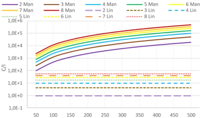
where R is the cell length, D is the reuse distance, and w is the street width. Figure 3 shows the comparison of the variation of

C/I with R between the two cases (user equipment at position 1,

i.e., cell edge, and at position 2, i.e., street crossing edge, at a distance w/2 of the eNB) while considering different reuse factors, rcc=D/R=2K. Although the first case also corresponds to a Manhattan grid, we label it as “Lin” (Linear) because the respective equations are formally the same as in the linear topology with cigar shaped cells. In the view chart, the number before “Man” or “Lin” represents rcc. C/I is higher when the user is at position 2 compared with the case where the UE is at position 1 (corresponding to the same equations for C/I as in the linear topology). As the worst-case occurs if the user is at position 1, we have considered the frequency reuse at distances

D-R and D+R, which in practice corresponds to considering the

linear topology.

Fig. 3. Variation of C/I with R, for the linear (“Lin”) and Manhattan (“Man”) topologies, while considering different reuse factors (rcc = D/R).

III. CNIR AND PHYSICAL THROUGHPUT

It is worthwhile to analyse the variation of the CNIR and Physical Throughput with the distance, d (0 ≤ d ≤ R) while understanding the behaviour of the system equivalent throughout. The underlying implicit formulation (from [9]) maps the CNIR onto the values of the PHY supported throughput, Rb, through the corresponding MCS, as shown in Figure 4, where the index J represents the MCS index. Figure 5 presents the variation of CNIR and Rb with the distance, d, for  ≠ 0, R= 50 m and different frequencies. The slight difference in the formulation consists on the fact that we are now considering linear cells in which the area is proportional to R; whereas in hexagonal cells (considered in [9]), the hexagonal crowns areas, corresponding to each individual MCSs, the area is proportional to R2_{. Tables I and II show the parameters considered in the}

computations. The standard deviation [db] is 0.004 for the 28

GHz frequency and 4.4 for 38, 60 and 73 GHz.

a) Correspondence of the PHY throughput for rings J, J -1, J -2, …, with the minimum CNIRs of consecutive MCS that map to step distances dJ, dJ-1, dJ-2, …

b) Areas of the coverage rings corresponding to a given PHY throughput. Fig. 4. Implicit formulation for the throughput (adapted from [8])).

1,0E-1 1,0E+0 1,0E+1 1,0E+2 1,0E+3 1,0E+4 1,0E+5 1,0E+6 50 100 150 200 250 300 350 400 450 500 C /I R

2 Man 3 Man 4 Man 5 Man 6 Man

7 Man 8 Man 2 Lin 3 Lin 4 Lin

Fig. 5. Variation of the CNIR and throughput with d for 28 GHz, 38 GHz, 60 GHz, 73 GHz, for R= 50 m for σ ≠ 0.

TABLE I. PARAMETERS CONSIDERED IN THE ANALYSIS (FROM [4])

Transmitter Power 0 dBW

Transmitter gain 3 dBi

Receiver gain 0 dBi

Carrier 20 MHz

Noise Figure 7 dB

Height (Base Station) 7 m Height (User Equipment) 1.5 m

TABLE II. VALUES FOR THE LOG-NORMAL RANDOM VARIABLE MINIMUM

CNIR, MODULATION AND SPECTRAL EFFICIENCY VERSUS MCS, FOR LTE, AND

VALUES FOR THE VERTICAL ASYMPTOTE FOR DL FROM 3GPP36.213

MCS mapping Rb[Mbps]

Mod. index CNIRmin[dB] Modulation ITBS Seff 20 MHz

1 -4.63 0 0.23 2.797 2 -3.615 1 0.31 3.624 3 -2.6 2 0.38 4.584 4 -1.36 3 0.49 5.736 5 -0.12 QPSK 4 0.6 7.224 6 1.17 5 0.74 8.76 7 2.26 6 0.88 10.296 8 3.595 7 1.03 12.216 9 4.73 8 1.18 14.112 10 6.13 9 1.33 15.84 11 7.53 9 1.33 15.84 12 8.1 10 1.48 17.568 13 8.67 11 1.7 19.848 14 9.995 16-QAM 12 1.91 22.92 15 11.32 13 2.16 25.456 16 12.78 14 2.41 28.336 17 14.24 15 2.57 30.576 18 14.725 15 2.57 30.576 19 15.21 16 2.73 32.856 20 16.92 17 3.03 36.696 21 18.63 18 3.32 39.232 22 19.975 19 3.61 43.816 23 21.32 64-QAM 20 3.9 46.888 24 22.395 21 4.21 51.024 25 23.47 22 4.52 55.056 26 25.98 23 4.82 57.336 27 28.49 24 5.12 61.664 28 31.545 25 5.33 63.776 29 34.6 26 5.55 75.376

Results for R = 25 and 100 m with  ≠ 0 and  = 0 are presented in [9]. It is worthwhile to note that the CNIR, hence

Rb, decreases from the 28 GHz to the 38 GHz frequency band, and then to the 60 and 73 GHz ones for coverage distances of up to circa 115 m. Then, there is a trend for the relative behaviour between the 60 GHz and 73 GHz frequency band (due to the reduction of the coverage owing to the O2 attenuation excess),

and the 60 GHz frequency band will have worst cellular coverage than the 73 GHz one.

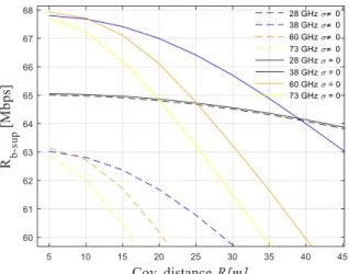
IV. ANALYSIS OF PHYTHROUGHPUT AND SYSTEM CAPACITY By applying the formulation for the computation of the equivalent supported throughput from [9], Chapter 9, p. 380, we obtain the curves for the supported throughput as a function of the coverage distance (not d) for the different frequency bands. We compare the cases where R varies between 25 and 500 m with the case where R varies between 5 and 100 m. We consider LTE-U parameters adapted to millimetre waves.

In Figures 6 and 7, R varies up to 100 and 500 m, respectively, for  = 0 and  ≠ 0. In these curves, it is clear that, in general, the supported throughput is higher for the 28 GHz frequency band compared to 38 GHz but the 60 GHz frequency band only performs better than the 73 GHz band for Rs up to approximately 100 m. Therefore, the throughput for the 73 GHz frequency band is higher. This is due to the O2 attenuation excess

which causes a reduction in the coverage at 60 GHz.

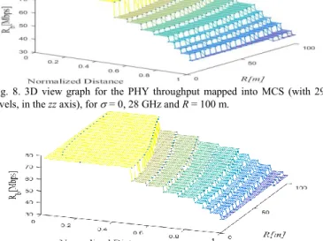
In order to study the influence of different frequency bands in the results for system capacity as a function of R, three dimensional (3D) graphs have been drawn, where the behaviour of the PHY throughput (Rb) mapped into MCS (with 29 levels, in the zz axis) is represented, as shown in Figures 8 and 9 (R=100 m). The cell size (R) varies from 5 m to 100. As in [10], [11], due to the range of distances d is different while cell radii vary from (0 ≤ d ≤ R), in the view charts we have considered the normalized distance, defined as d/R, when representing the stepwise behaviour of the PHY throughput that defines the ring area which is using a certain MCS within the cell.

Fig. 6. Supported throughput for 28 GHz, 38 GHz, 60 GHz, 73 GHz, and R=100 m, for σ = 0 and σ ≠ 0.

Fig. 7. Supported throughput for 28 GHz, 38 GHz, 60 GHz, 73 GHz, and R=500 m, for σ = 0 and σ ≠ 0.

Fig. 8. 3D view graph for the PHY throughput mapped into MCS (with 29 levels, in the zz axis), for = 0, 28 GHz and R = 100 m.

Fig. 9. 3D view graph for the PHY throughput mapped into MCS (with 29 levels, in the zz axis), for ≠ 0, 28 GHz and R = 100 m.

The normalized distance represents the variation of d from 0 to R. The cell ranges are represented in the yy axis while the normalized distance is shown in the xx axis and varies from 0 to 1. By analysing these surfaces of the PHY throughput, it can be understood that the decrease in the MCSs, while the distance varies inside the cell, is faster for longer Rs and an interpretation of the behaviour for the different frequency bands is possible. Results are clearly better for  = 0 compared to the case  ≠ 0 (when the fading margin is considered for coverage purposes).

V. COST/REVENUE TRADE-OFF

Concerning to the enhancement of the system from the profit point of view, we compute from throughput the results for cost and revenues, using the model described in [12], [13]. The scenario presented in Figure 4, behaves similarly to a Manhattan geometry outdoor environment, through the respective linearization described in Section I and Figure 1, with omni-directional cells and antennas.

The overall cost of the network per unit length, per year, C0[€/ul],

is given by

𝐶0 €/𝑢𝑙 = 𝐶𝑓𝑖€/𝑢𝑙 +𝐶𝑓𝑏⋅ 𝑁𝑐/𝑢𝑙 (5)

where Cfi is a fixed term cost, Cbf is cost proportional to the number of BSs, and the number of cells per unit area is given by 𝑁𝐶/𝑢𝑙= 1 2. 𝑅 𝑘𝑚 − 𝑤 𝑘𝑚 2 (6)

It is worthwhile to note that the building block dimensions change with R, since the side length is (2R-w), causing a variation in the streets area, what does not occur in reality. However, the linearized curves of costs and profits of the network, shown in Figures 10 to 11 are not affected, since only the street length is considered, instead of the area [12], [13]. The revenues per cell, (Rv)/cell[€], can be attained as a function of the throughput per Base Station, BS, thrBS[kbps], and the revenue of a channel with a data rate Rb[kbps], Rrb[€/min], and Tbh

corresponding the equivalent duration of busy hours per day [12], Rv/cell[€] can be obtained by

𝑅𝑣 𝑐𝑒𝑙𝑙 € =

thr𝐵𝑆 𝑘𝑏𝑝𝑠 ∙ 𝑇𝑏ℎ∙ 𝑅𝑟𝑏 €/𝑚𝑖𝑛

𝑅𝑏 𝑘𝑏𝑝𝑠

(7)

Revenues are considered in annual basis, where we considered six busy hours per day, 240 busy days per year [10], and the price of a 144 kbps “channel” per minute (corresponding to the price of ≈ 1 MB), considering R144

kbps[€/min] =0.07. Considering the throughput with σ ≠ 0 in order

to obtain more realistic values. The revenue per cell can be obtained by

𝑅𝑣 𝑐𝑒𝑙𝑙 € =

thr𝐵𝑆 𝑘𝑏𝑝𝑠 ∙60∙6∙240∙𝑅𝑟𝑏 €/𝑚𝑖𝑛

144 𝑘𝑏𝑝𝑠

(8) Figure 12 presents results for the revenue per cell per year, with Rb=144 kbps, through variation of R for Rmax=100 m. It is evident that 28 GHz band is the most profitable of all bands for all distances and the profit will be lower as the distance increases for all frequencies.

Fig. 10. Revenue per cell with Rb=144 kbps and 5 ≤R ≤ 100 m.

Fig. 11. Revenue per cell with Rb=144 kbps and 5 ≤R ≤ 500 m.

Fig. 12. Network revenue/cost per unit length per year as a function of R, with

The revenue per unit area per year, Rv, is obtained multiplying the revenue per cell by the number of cells per unit of area, as follows 𝑅𝑣 €/𝑘𝑚 = 𝑁𝑐/𝑢𝑙𝑎. 𝑅𝑣 𝑐𝑒𝑙𝑙 € (9) 𝑅𝑣 €/𝑢𝑙𝑎 = 1 2.𝑅 _𝑘𝑚 −𝑤 𝑘𝑚 2 . thr𝐵𝑆 𝑘𝑏𝑝𝑠 .𝑇𝑏ℎ.𝑅𝑟𝑏 €/𝑚𝑖𝑛 𝑅_{𝑏 𝑘𝑏𝑝𝑠} (10) Cfb is given by 𝐶𝑓𝑏 € = 𝐶𝐵𝑆+ 𝐶𝐼𝑛𝑠𝑡 𝑁𝑦𝑒𝑎𝑟 + 𝐶𝑀&𝑂 (11)

Cfbcan be calculated by assumption present in Table III, for five-year project duration, assuming unlicensed bands.

In a near future, with the equipment normalization and mass production, the equipment prices will get lower, making this kind of communication more accessible comparable to the modem “normal prices”, like “Qualcomm Snapdragon X50” modem. Qualcomm, according to the “Snapdragon X50 5G” modem is capable of download speeds of up to 5 Gbps which is five times faster than the fastest 4G modem [14], [15].

The profit, Pft, is an important outcome to enhance the network, and is given by the difference between the revenues and the costs in €/km, while the profit in percentage is given by the net revenue normalized by the cost

𝑃𝑓𝑡 €/𝑘𝑚 = 𝑅𝑣 €/𝑘𝑚 −𝐶0 €/𝑘𝑚 /𝐶0 €/𝑘𝑚 (12)

We consider the profit in percentage instead of the absolute profit because this metric is more relevant for operators and service providers [13]. If Rv [€/km]-C0[€/km] is positive, there will

be profit. Figures 13 and 14 present the results for the overall cost per unit length per year, C0, and the revenue per unit length

per year, for only one carrier. For our assumptions, the revenues are noticeably higher than the costs of all frequencies. Some curves are overlapped showing similar revenues. Considering all the computation with the respective price per minute and all the costs from Table III, for 60 and 73 GHz frequency bands, for distances longer than 210 m and 245 m, respectively, and for 38 GHz frequency band with distances above 440 m, the system is not profitable. For all studied distances, 28 GHz is the only profitable frequency band for the longest coverage distances. For distances between 5 m and 20 m the profit is higher than 240% at 28 GHz and 220% for the remaining frequencies.

For the 60 and 73 GHz bands, as shown in Figures 17 to 18, the average profit is similar for all range of Rs, while for distances longer than 130 m the profit for the 73 GHz band is higher due to the highest system capacity (as the extra O2

attenuation additionally affects coverage at 60 GHz). TABLE III. ASSUMPTIONS FOR BASE STATION COSTS FROM [12]

Parameters Values [€] Initial costs: BS price, CBS Installation, CInst Fixed, Cfi Annual Cost: Operation and maintenance, CM&O 2500 250 0,unlicensed bands 250

Fig. 13. – Profit per unit length per year, in percentage with Rmax = 100 m.

Fig. 14 – Profit per unit length per year, in percentage with Rmax = 500 m. The results clearly indicate that coverage distances up to 80 m should be used to optimise the system by having into consideration the maximization of the profit in percentage. As the goal of operators and service providers is to enhance the profit, where the profitable zone is for short distances mainly in the 28GHz frequency band, from 5 to 80 m.

VI. CONCLUSION

In this study, we identify and discuss the potentialities of mobile cellular communications in the millimetre wavebands, showing that very high bit/data rates can be supported in small cells with short-range coverage. As in real environments, cellular mobile communications are simultaneously affected by noise and co-channel interference, we have studied the behaviour of the carrier-to-noise-plus-interference ratio with the coverage distance (and the actual distance from users to the eNBs) while analysing its impact in cellular planning and the optimization process. Foremost, for =2.3 (40 and 60 GHz), the carrier-to-interference ratio (C/I) is increasing with R and is clearly higher when the co-channel reuse factor rcc=D/R raises from 2 to 8. C/I is higher when the user is at position 2 compared with the case where the UE is at position 1 corresponding to the worst-case in the linear topology.

The equivalent supported throughput within cells was assessed while considering reuse pattern K = 2, assuming in this preliminary phase that LTE is considered, but other air interfaces will also be assumed. In terms of cell coverage and the computation of interference, LoS propagation models have been considered at the 28, 38, 60 and 73 GHz bands.

From these analytical computations, we have learned that the highest system capacity and the highest modulation coding schemes are achieved for coverage distances up to 30 m. Likewise the supported throughput decreases for the longest coverage ranges and it is clearly more favourable for the lowest

frequency bands. However, in terms of interference the system shows highest interference for lowest frequency bands.

For  =0, the 38, 60 and 73 GHz frequency bands only performs better than 28 GHz frequency band for Rs up to 20 m, 25 m, 38 m for, 73, 60 and 38 GHz respectively as shown Figure 15. For  ≠ 0, In general, the supported throughput is higher for the 28 GHz frequency band, which always becomes higher than the values for the other frequency bands, ([dB] = 0.004 at 28

GHz and [dB] =4.4 for at 38, 60 and 73 GHz) for the whole

range of coverage distances, showing that the better the coverage is the higher the system capacity becomes, although the system capacity is inferior for  ≠ 0.

Fig. 15 – Zoomed plot from figure 7, Supported throughput for 28 GHz, 38

GHz, 60 GHz, 73 GHz, for σ = 0 and σ ≠ 0.

The 60 GHz frequency band only performs better than the 73 GHz band for Rs up to approximately 115 m. After this distance, the throughput for the 73 GHz frequency band is higher. This fact is due to the O2 attenuation excess which

results in the reduction of the coverage at 60 GHz, yielding lower values for the supported throughput.

In our scenario, the profit is mostly a decreasing function with R. Consequently, the most profitable cell radii are the lowest ones for all frequencies, and the best behaviour occurs in the 28 GHz band. For long distances, the system ceases to be profitable. Revenues are proportional to the supported throughput. Computations show that, in the future, it is possible to install these types of structure when costs of installation and maintenance the network decreases, enabling higher system capacity while reducing prices. The optimum values for the profit in percentage are obtained in the range R ≈ 5m to R ≈ 20m, with profit near to 240%. The results clearly indicate that coverage distances up to 80 m should be used to optimise the system in terms of profit.

ACKNOWLEDGMENT

Authors would like to thank Sofia Sousa and Rui Paulo for the unconditional support.

REFERENCES

[1] F. J. Velez, M. Dinis and J. Fernandes, “Mobile Broadband Systems: Research and Visions,” IEEE VTS (Vehicular

Technology Society) News, Vol. 52, No.2, May 2005.

[2] T.S. Rappaport et al., "Millimeter Wave Mobile Communications for 5G Cellular: It Will Work!", IEEE

Access, vol. 1., pp. 335-349, May 2013.

[3] J.M. Brázio and F.J. Velez, “Design of Cell Size and Frequency Reuse for a Millimetrewave Highway Coverage Cellular Communication System,” in Proc. of PIMRC’96 - 7th

IEEE International Symposium on Personal Indoor, and Mobile Communications, Taipei, Taiwan, ROC, Oct. 1996.

[4] T. S. Rappaport, R. W. Heath and R. Daniels, and J. Murdock,

Millimeter wave wireless communications, Prentice Hall,

Pearson Education, Upper Saddle River, NJ, USA, 2014. [5] M. K. Samimi, T. S. Rappaport, and G. R. MacCartney,

“Probabilistic omnidirectional path loss models for millimeter-wave outdoor communications,” IEEE Wireless

Communicat. Letters, vol. 4, no. 4, Aug. 2015, pp. 357-360.

[6] A. I. Sulyman, A. T. Nassar, M. K. Samimi, G. R. Maccartney, T. S. Rappaport and A. Alsanie, “Radio propagation path loss models for 5G cellular networks in the 28 GHz and 38 GHz millimeter-wave bands,” IEEE

Communicat. Magazine, vol. 52, no. 9, Sept. 2014., pp.78-86

[7] T. S. Rappaport, G. R. MacCartney, M. K. Samimi and S. Sun, “Wideband Millimeter-Wave Propagation Measurements and Channel Models for Future Wireless Communication System Design,” IEEE Transactions on

Communications, vol. 63, no. 9, Sept. 2015, pp. 3029-3056.

[8] F. J. Velez and L. M. Correia, J. M. Brázio, “Frequency Reuse and System Capacity in Mobile Broadband Systems: Comparison between the 40 and 60 GHz Bands,” Wireless

Personal Communications, vol.19, no. 1, Aug. 2001, pp.1-24.

[9] E. S. B. Teixeira, S. Sousa, R. R. Paulo and F. J. Velez, “Frequency Reuse Trade-off and System Capacity in Small Cell Networks in the Millimetre Wavebands,” 3rd _{Meeting of}

the Management Committee of COST CA 15104 - IRACON, TD(17)04084, Lund, Sweden, May 2017.

[10] R. Prasad and F. J. Velez, WiMAX Networks:

Techno-economic Vision and Challenges, Springer, Dordrecht, The

Netherlands, 2010.

[11] S. Sousa, F. J. Velez, J. M. Peha, “Impact of considering the ITU-R Two Slope Propagation Model in the System Capacity Trade-off for LTE-A HetNets with Small cells,” in Proc. of

32nd URSI GASS 2017, Montreal, Canada, Aug. 2017.

[12] F. J. Velez, and L. M. Correia. "Optimisation Of Mobile Broadband Multi-Service Systems Based In Economics Aspects," Wireless Nets. vol.9, no. 5, Sep 2003: pp. 525-533. [13] F. J. Velez, O. Cabral, F. Merca, V. Vasos. Service characterization for cost/benefit optimization of enhanced UMTS. Telecom. Systems vol. 50, no. 1, Apr 2012, pp 31-45. [14] J. Gozalvez, "5G Worldwide Developments [Mobile Radio]," in IEEE Vehicular Technology Magazine, vol. 12, no. 1, March 2017, pp. 4-11.

[15] Qualcomm.(2017, October). Networks (2nd ed.) [Online]. Available:https://www.qualcomm.com/products/snapdragon/ modems/5g/x5 [16] Forbes(2017,October).[Online].https://www.forbes.com/sites /patrickmoorhead/2016/10/17/qualcomm-unveils-the- worlds-first-5g-modem-snapdragon-x50-for-28-ghz-mmwave-networks/#b2c5f655a670