WO R K I N G PA P E R S E R I E S
N O. 5 8 1 / J A N UA RY 2 0 0 6
PUBLIC SECTOR
EFFICIENCY
EVIDENCE FOR NEW EU
MEMBER STATES AND
EMERGING MARKETS
In 2006 all ECB publications will feature a motif taken from the
€5 banknote.
WO R K I N G PA P E R S E R I E S
N O. 5 8 1 / J A N U A RY 2 0 0 6
This paper can be downloaded without charge from http://www.ecb.int or from the Social Science Research Network electronic library at http://ssrn.com/abstract_id=876945.
PUBLIC SECTOR
EFFICIENCY
EVIDENCE FOR NEW EU
MEMBER STATES AND
EMERGING MARKETS
1by António Afonso
2, 3,
Ludger Schuknecht
3and Vito Tanzi
4C O N T E N T S
Abstract 4
Non-technical summary 5
1. Introduction 7
2. Measuring efficiency in public expenditure: conceptual issues 8
2.1 Measuring costs 9
2.2 Efficiency with wrong goals 12
2.3 Efficiency with right goals 13
3. Measuring efficiency in public expenditure: methodologies 16
3.1 Composite indicators for measuring
public sector performance and efficiency 16
3.2 Non-parametric analysis of performance and efficiency 20
3.3 Using non-discretionary factors to
explain inefficiencies 23
4. A quantitive assessment of public sector
performance and expenditure efficiency 24
4.1 Some stylised facts for the EU new
member states and comparative countries 24
4.2 Public sector performance and efficiency via composite indicators 29
4.2.1 Public sector performance (PSP) 30
4.2.2 Public sector efficiency (PSE 32
4.3 Relative efficiency analysis via a DEA
approach 34
4.4 Explaining inefficiencies via
non-discretionary factors 39
5. Conclusion 41
References 43
Annex – Data and sources 46
Abstract
In this paper we analyse public sector efficiency in the new member states of the European Union compared to that in emerging markets. After a conceptual discussion of expenditure efficiency measurement issues, we compute efficiency scores and rankings by applying a range of measurement techniques. The study finds that expenditure efficiency across new EU member states is rather diverse especially as compared to the group of top performing emerging markets in Asia. Econometric analysis shows that higher income, civil service competence and education levels as well as the security of property rights seem to facilitate the prevention of inefficiencies in the public sector.
Keywords: government expenditure, efficiency, DEA, new EU member states, emerging markets.
Non-technical summary
The importance of the efficient use of public resources and high-quality fiscal policies
for economic growth and stability and for individual well-being has been brought to the
forefront by a number of developments over the past decades. Macroeconomic constraints
limit countries’ scope for expenditure increases. The member states of the European Union
are bound to fiscal discipline through the Stability and Growth Pact. Globalisation makes
capital and taxpayers more mobile and exerts pressure on governments’ revenue base. New
management and budgeting techniques have been developed and there is more scope for
goods and service provision via markets. Transparency of government practices across the
globe has increased, raising public pressure to use resources more efficiently.
Our contribution in this study is essentially threefold: first we discuss and survey
conceptual and methodological issues related to the measurement and analysis of public
sector efficiency. Second we construct Public Sector Performance and Efficiency composite
indicators for the ten new member states that acceeded to the European Union (EU) on 1 May
2004 as compared to emerging markets from different regions, future EU candidate countries
and some current EU member countries that show features of emerging markets and/or are
undergoing a catching up process. Third we use Data Envelopment Analysis to compute input
and output efficiency scores and country rankings, which we combine with a Tobit analysis to
see whether exogenous, non-discretionary factors play a role in explaining expenditure
inefficiencies. To our kowledge, such an efficiency analysis has not been applied before to
this set of countries.
The Public Sector Performance and Efficiency composite indicator includes
information on administrative, education, health, income distribution, economic stability, and
economic performance outcomes. It is interesting to see that a relatively strong performance
of the new EU member states on human capital/education and income distribution contrasts
with a relatively weak one for economic performance and stability. There is no clear pattern
of distinction between Baltic and Central European countries while the two island countries
post strong values for all indicators for which data is available. Asian Emerging economies
performed very strongly on administration, human capital and economic stability and growth.
The results of our analysis show that expenditure efficiency across new EU member
states is rather diverse, especially compared to the group of top performing emerging markets
in Asia. From the analysis of composite public sector performance (PSP) and efficiency (PSE)
scores we find that countries with lean public sectors and public expenditure ratios not far
from 30% of GDP tend to be most efficient. PSE scores of the most efficient countries are
more than twice as high as those of the poorest performers.
From the DEA results we see that a small set of countries define, or are very close to,
the theoretical production possibility frontier: Singapore, Thailand, Cyprus, Korea, and
Ireland. From an input perspective the highest ranking country uses 1/3 of the inputs as the
bottom ranking one to attain a certain public sector performance score. The average input
scores suggest that countries could use around 45 per cent less resources to attain the same
outcomes if they were fully efficient. Average output scores suggest that countries are only
delivering around 2/3 of the output they could deliver if they were on the efficiency frontier.
Finally we examine via Tobit analysis the influence of non-discretionary factors,
notably non-fiscal variables, on expenditure efficiency. Our analysis suggests that the security
of property rights, per capita GDP, the competence of civil servants, and the education level
of people positively affect expenditure efficiency. Due to significant correlation, however, the
two competence/education variables are only significant in separate regressions while the
other two variables are robust over all specifications. International trade openness, trust in
politicians and transparency of the political system have not been found to display a
significant influence on expenditure efficiency (even though only the coefficient for public
I. Introduction
The importance of the efficient use of public resources and high-quality fiscal policies
for economic growth and stability and for individual well-being has been brought to the
forefront by a number of developments over the past decades. Macroeconomic constraints
limit countries’ scope for expenditure increases. The member states of the European Union
are bound to fiscal discipline through the Stability and Growth Pact. Globalisation makes
capital and taxpayers more mobile and exerts pressure on governments’ revenue base. New
management and budgeting techniques have been developed and there is more scope for
goods and service provision via markets. Transparency of government practices across the
globe has increased, raising public pressure to use resources more efficiently (see also Tanzi
and Schuknecht (2000), Heller (2003), Joumard, Konsgrud, Nam and Price (2004)).
The adequate measurement of public sector efficiency is a difficult empirical issue and
the literature on it, particularly when it comes to aggregate and international data, is rather
scarce. The measurement of the costs of public activities, the identification of goals and the
assessment of efficiency via appropriate cost and outcome measures of public policies are
very thorny issues. Academics and international organisations have made some progress in
this regard by paying more attention to the costs of public activities via rising marginal tax
burdens and by looking at the composition of public expenditure. Moreover, they have been
shifting the focus of analysis from the amount of resources used by ministry or programme
(inputs) to the services delivered or outcomes achieved (see, for instance, OECD (2003),
Afonso, Ebert, Thöne and Schuknecht, (2005), and Afonso, Schuknecht and Tanzi (2005)).
Our contribution in this study is essentially threefold: first we discuss and survey
conceptual and methodological issues related to the measurement and analysis of public
sector efficiency. Second we construct Public Sector Performance and Efficiency composite
indicators for the ten new member states that adhered to the European Union (EU) on 1 May
2004 as compared to emerging markets from different regions, future EU candidate countries
and some current EU member countries that show features of emerging markets and/or are
undergoing a catching up process.1 Third we use Data Envelopment Analysis to compute
input and output efficiency scores and country rankings, which we combine with a Tobit
1
analysis to see whether exogenous, non-discretionary (and non-fiscal) factors play a role in
explaining expenditure inefficiencies.2 To our kowledge, such an efficiency analysis has not
been applied before to this set of countries.
On the second and third objective, the study finds significant differences in
expenditure efficiency across new member countries with the Asian newly industrialised
economies performing best and the new member states showing a very diverse picture. The
econometric study shows that income, public sector competence and education levels as well
as the security of property rights seem to facilitate the prevention of inefficiencies in the
public sector.
The paper is organised as follows. In section two we discuss conceptual issues
regarding public expenditure efficiency. In section three we present the methodologies used
for the measurement of public expenditure efficiency. Section four reports stylised facts
regarding the new EU member states and various ways for assessing public sector efficiency:
via i) performance and efficiency analysis based on cross-country composite indicators, ii) a
parametric efficiency analysis, and iii) an explanation of inefficiencies via
non-discretionary factors. Section five concludes.
II. Measuring efficiency in public expenditure: conceptual issues
Economists are concerned about the efficient use of scarce resources. The concept of
efficiency finds a prominent place in the study of the spending and taxing activities of
governments. Economists believe that these activities should generate the maximum potential
benefits for the population and they castigate governments when, in their view, they use
resources inefficiently. International organisations, such as the World Bank and the IMF,
often express concern about governmental activities that they consider inefficient or
unproductive.
Like the proverbial elephant, efficiency or, more often inefficiency, is easier to
recognize than to define objectively and precisely. Merriam Webster reminds us that
2
efficiency has to do with the comparison between input, and output or between costs and
benefits. At a given input, the greater the output, the more efficient an activity is. A machine
is efficient when, at a given cost, it produces the largest possible output. For example, a
furnace is efficient when it produces a good amount of heat at a given cost. A car is efficient
when it goes a good number of miles with a gallon of gasoline.
The measurement of efficiency generally requires: (a) an estimation of costs; (b) an
estimation of output; and (c) the comparison between the two. Applying this concept to the
spending activities of governments, we can say that public expenditure is efficient when,
given the amount spent, it produces the largest possible benefit for the country’s population.
Here the word benefit is used because economists often make a distinction between output
and outcome, a distinction to which we shall return later.
Often efficiency is defined in a comparative sense: the relation between benefits and
costs in country A is compared with that of other countries. This can be done for total
government expenditure, or for expenditure related to specific functions such as health,
education, poverty alleviation, building of infrastructures and so on. If in country A the
benefits exceed the costs by a larger margin than in other countries, then public expenditure in
country A is considered more efficient.
The simple comparison outlined above requires that both costs and benefits be
measured in acceptable ways. This is easy, or easier, for machines (cars, furnaces) but
difficult for governmental activities. It is often difficult to measure the benefits from a
governmental expenditure. But, one could assume that, at least the costs (i.e., the resources
used) should be easy to determine. Unfortunately, this is not always so. Deficient budgetary
classifications, lack of reliable data, difficulties in allocating fixed costs to a specific function,
and failure to impute some value to the use of public assets used in the activity can also
hamper the determination of real costs.
II.1. Measuring costs
A problem that arises from the comparison of, say, the efficiency of a car or a furnace
with that of public spending is that additional amounts of inputs such as gasoline, petroleum
other words it is possible to assume a perfectly elastic supply curve for the input used by an
individual. This, however, is not the case for public spending. Public spending is financed by
tax revenue and more revenue can be obtained only at progressively higher marginal costs.
It is a well established conclusion, supported by both theory and empirical work, that,
once a tax administration is in place, the marginal cost of tax revenue is generally higher than
the average cost, and that marginal costs can increase rapidly. This is true in all countries but
perhaps more so in emerging markets and developing countries. These countries face great
difficulties in establishing good and efficient tax systems. As a consequence, they must often
rely on revenue sources that impose: (a) dead weight costs, because of the distortions and the
disincentives that they impose on the economy; (b) high costs for the countries’ tax
administrations; and (c) high compliance costs for the taxpayers. Thus, the true cost to the
economy of the marginal dollar collected in taxes can significantly exceed the dollar received
by the government. The assumption of a perfectly elastic supply curve for tax revenue is not
tenable.
Each additional dollar of spending, requiring an additional dollar of revenue, will
impose additional and rising marginal costs on the economy unless that dollar comes from
reducing some other spending. The concept of efficiency in public spending must take this
into account. Both the level of taxation and the quality of the tax system should become
essential elements for the evaluation of the efficiency of public spending. This is quite apart
from whether the use to which the tax revenue is put is efficient or not. An analysis that
focused only on the use of revenue would be missing these important aspects.
A simple graphical presentation can explain more formally this important, obvious,
but often-ignored point. It is made ignoring, for the time being, the efficiency in the actual use
of the tax revenue. The focus, here, is on the efficiency in the tax collection side.
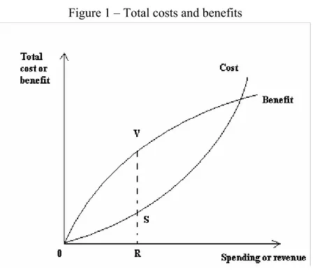
In Figure 1, the vertical axis measures both the benefits from public expenditure to the
country’s population and the costs imposed by the taxes collected. It is assumed that the same
unit of measurement can be used to measure both. The vertical axis reflects total benefits from
public expenditure and total costs of taxation. These costs include, in addition to the monetary
When the tax administration is corrupt, they include also bribes paid by the taxpayers to the
corrupt tax administrators.
Figure 1 – Total costs and benefits
The budgetary or monetary value of public expenditure and the tax revenue to cover
the expenditures are both measured, in dollars, on the horizontal axis. More public
expenditure is supposed to bring more benefits to the population. Thus the curve is positively
sloped. However, the marginal benefit from each additional dollar spent can be expected to
fall as more dollars are spent. Thus, the curve that reflects total benefits is concave downward,
i.e., its second derivative is negative. Curve OVB in Figure 1 describes this behaviour.
As more taxes are collected, each additional dollar collected becomes more costly.
Therefore, the curve, OSC, describing the total costs of taxation is concave upward, i.e., its
second derivative is positive.
At a level of public expenditure equal to OR, the slopes of the two curves are equal
which means that the true cost of the last dollar spent is exactly equal to the benefit created by
that spending. Before point R, increasing tax revenue and public spending increases net
benefits which are measured by the vertical distance of the two curves. Beyond point R, the
marginal cost of taxation exceeds the marginal benefits from spending. VS is the largest
There are other reasons why the budgetary costs of an activity can underestimate the
true costs of the activity. We shall mention two such reasons. The first is that most
governments do not consider in their budgetary estimates of the costs of particular activities
(education, defence, etc.) the opportunity costs of using government-owned assets such as
buildings, land, forests and so on. For example the budgetary cost of a school includes the
costs of teachers’ salaries, school equipment and so on but it often does not include the rental
value of the government-owned building used. The same is true for the cost of jails, for the
cost of military bases, to name a couple of examples. This means that the budgets, and
especially those for particular categories of spending, often, and at times substantially,
underestimate, the true costs of these activities.3
Still another reason for the underestimation of the costs of particular activities is the
difficulty of allocating government fixed costs among the particular activities. When, for
example, the educational budget is considered in relation to the benefits from the spending,
that budget will not include any part of the fixed costs of running a government. These costs
for example should include parts of the activities of parliaments, the president’s office and so
on.
II.2. Efficiency with wrong goals
It is difficult to recognize in the analysis of efficiency in public expenditure that
expenditure can be efficient in a technical sense – i.e. the goal pursued is pursued at low cost
– but nevertheless can be inefficient in the sense of public interest or social welfare. This
occurs when the government efficiently produces the wrong output. This is the classic case of
guns versus butter. A government may be producing public defence efficiently but it may be
producing too much of it (too many guns) and too little of other social goods (health,
education) compared to what the population would prefer to have.
This is clearly a political problem. In a democratic society that operates well with
checks and balances at the political level, the executive branch, under the control of a
democratically elected parliament, determines the size and the composition of the budget.
This budget can be assumed to reflect legitimately the goals of the population. In this case,
3
the main question is the technical one of how efficiently the money assigned to each function
is being spent. Thus, we could talk about technical inefficiency and not about political, or goal
related, inefficiency.
Unfortunately, much of the world is not made up of well functioning democracies.
The problem of “state capture” is a common one and one that has received much attention on
the part of the World Bank. But even when “state capture” is not a problem, powerful lobbies
and corruption can divert the budget towards goals that are not identical with those that would
reflect the public interest. In these situations the definition of efficiency becomes less clear.
In conclusion it is important to recognize the distinction between producing the wrong
output (i.e. allocating the budget to the wrong activities) but spending the money in a
technically efficient (i.e. low cost) way; and allocating the budget to the right activities (i.e. so
much for health, so much for education, etc) but doing it in an inefficient (i.e. high cost) way.
Both of these problems are common and important, and both lead to inefficiency in the use of
resources. Unfortunately in many situations one finds both problems, that is, the wrong output
is produced and it is produced in an inefficient way.
II.3. Efficiency with right goals
In the previous sub-section we have discussed the possibility that, for various reasons,
the budget gets distorted towards goals (defence, etc.) that the majority of the population may
see as lower priorities than socio-economic goals such as health, education, support for poor
groups, high growth and so on. Suppose, however, that the budget allocates proportions that
may be considered appropriate toward popular expenditures such as health and education. UN
Guidelines have at times recommended that governments allocate specific proportions of their
budgets to particular social functions. In these situations various problems may arise that
would tend to make the public spending less efficient than it could be. Let us mention some of
these problems.
First, a problem similar to the one mentioned in the previous section is the hijacking of
the expenditure for the specific benefit of special pressure groups. For example educational
spending may be redirected from primary education towards secondary or tertiary education
from prevention to hospital care; or from rural to urban areas; or from basic health to modern
hospitals in big cities; or the resources may be allocated from diseases that affect mostly
poorer people, such as malaria toward old people or “higher income” diseases. These
redirections within a budgetary category are often important in determining the benefits that
come out from the expenditure for a basic function; they are important in determining
efficiency even when they do not change the total amounts spent for the category.
Second, and a problem that has attracted little attention, is the administrative hijacking
of the budgeted resources by the provider of the services. For certain public functions and
especially for those that are labour-intensive, such as education and health, the role of the
providers of the services, (school teachers, administrators, doctors, nurses and so on) is
fundamental. Unlike cash transfers (as for the payment of pensions) that are received directly
by the legal beneficiaries, much of the actual spending for activities such as education and
health goes to the salaries of the public employees that provide the services. In exchange for
the salaries received these employees are supposed to produce an output in the form of
services that benefit patients, school children and other users in terms of good health, more
literacy, more human capital and so on.
There has been a tendency among economists to measure the output or the benefit in
these activities on the basis of the budgeted allocation: the higher the expenditure, the higher
the benefit. For example calls to allocate a given, or a larger, share of national budgets to
health and education assume the identity between expenditure and benefits. The larger the
expenditure, the greater the benefits received by the intended destinatories are assumed to be.
But, as argued already by Tanzi a long time ago (1974) the two can be widely different. This
difference is central to the concept of efficiency.
Health, education and similar activities absorb a large share of the government payroll
and the personnel who work for the government. Through high salaries they can absorb a
large share of the budget allocated to these activities thus leaving little for ancillary needs.
This is especially the case when those who work in these activities (school teachers, doctors,
nurses) are well organized politically. If mostly higher salaries absorb additional resources
allocated to these activities and the higher salaries are not accompanied by higher productivity
of the public employees, the higher public spending can be unproductive and produce little
countries. For example, Aninat at al. (1999) referred to the Chilean experience where a
tripling of the real public spending on health over a few years did not produce any visible or
measurable increase in the quantity or quality of the services to those who used the public
health system. The increase in spending simply resulted in rents for the doctors and/or nurses.
In other countries large increases in educational spending had little impact on educational
output.
In connection with the above point we need to return to the question of the distinction
between output and outcome. This distinction should be fundamental in the analysis of the
efficiency of public spending. There is often much attention paid to the outputs of certain
activities and too little to the outcomes. For example the outputs of educational spending may
be school enrolments, or number of students completing a grade. The outputs of health
expenditure may be the number of operations performed or days spent in a hospital bed.
However, the outcomes should be based on how much students learned and how many
patients got well enough to return to a productive life.
Third, corruption in its various forms has a deleterious effect on public expenditure
efficiency or productivity. Corruption may be linked to the existence of ghost workers, i.e.
individuals who receive a salary from the government but who never show up on the job; or,
in some extreme cases, are literally inexistent. It may be linked to individuals who have
double jobs and who spend as little time and energy at the government job as possible. It may
be linked to individuals who often do not show up in their jobs claiming illness or some other
reasons. It may be linked to the assignment of incompetent individuals in sensitive jobs or to
overstaffing and nepotism, and so on. There is little question that corruption and inefficiency
are often two sides of the same coin so that reduction of corruption becomes a sine qua non
for an increase in efficiency. However, the effect of corruption is more likely to be noted in
outcomes then in outputs of public spending.
Finally, what we call inefficiency may be the result of cultural factors, such as attitude
toward work; climatic factors, that make it difficult to work in certain periods, such as
summers, afternoons, etc.; traditions, such as number and length of religious holidays, and so
on. These factors may generate what, borrowing a term from the economic development
literature, could be called an X-inefficiency factor, which is difficult to define and measure
III. Measuring efficiency in public expenditure: methodologies
III.1. Composite indicators for measuring public sector performance and efficiency
In recent years various attempts have been made at measuring the efficiency of public
expenditure via composite indicators. These attempts are of two broad types: macro
measurements, and micro measurements. Macro measurements aim at estimating the
efficiency of total public spending. Micro measurements aim at measuring the efficiency of
particular categories of public spending. These methods try to make progress in tackling the
most important measurement challenges: they aim to identify appropriate objectives, they
measure outcomes of public sector activities that proxy these objectives (rather than inputs),
and they set these in relation to the costs (expenditure and taxes).
Macro measurements have as their aim an evaluation of public spending in its entirety.
In other words they attempt to measure, or rather to get some ideas of, the benefits from
higher public spending. When, for example, Sweden spends 1 ½ times as much in terms of
GDP shares as Switzerland, what does it get in return? Micro measurements attempt to
determine the relationship between spending and benefits in a particular budgetary function or
even sub-function (i.e., health spending or the efficiency of spending in hospitals, or spending
for protection against malaria, aids, etc.).
A first and simple macro measurement attempt was made by Tanzi and Schuknecht
(1997, 2000) in trying to assess the benefits from total public spending in 18 industrialized
countries. The approach attempts to determine whether larger public spending in these
industrialized countries provided returns, in terms of some identifiable benefits, that could
justify the additional costs, including the limitation in individual economic freedom
associated with higher tax burdens, imposed by that additional spending. The key question
that it tries to address is whether there is a positive, identifiable relationship between higher
public spending and higher social welfare.
This approach is a comparative method which uses data on various socio-economic
indicators that are available for groups of countries. The countries are classified in terms of
values of, or the changes in, the socio economic indicators. The greater the positive impact of
higher spending on the indicators, the more efficient public expenditure is assumed to be.
The application of this method led the authors to conclude that additional public
expenditure had not been particularly productive in recent decades. The group of countries
with lower levels of public spending had socio-economic indicators that were as good as or at
times better than the countries with much higher spending levels.4
Afonso, Schuknecht, and Tanzi (2005) refined this approach and built composite
indicators of public sector performance. They distinguished public sector performance (PSP),
defined as the outcome of public policies, from public sector efficiency, defined as the
outcome in relation to the resources employed. This is also the first method we apply to the
new member and emerging market analysis later in the paper.
Assume that public sector performance (PSP) depends on the values of certain
economic and social indicators (I). If there are i countries and j areas of government
performance which together determine overall performance in country i, PSPi, we can then
write
∑
=
=
n j
ij
i PSP
PSP
1
, (1)
with PSPij = f(Ik).
Therefore, an improvement in public sector performance depends on an improvement
in the values of the relevant socio-economic indicators:
∑
=
∆ ∂
∂ = ∆
n k i
k k
ij I
I f
PSP . (2)
The performance indicators are of two kinds: process or opportunity indicators, and traditional
or Musgravian indicators. As a first step, they defined seven sub-indicators of public
4
performance. The first four look at administrative, education, health and public infrastructure
outcomes. Each of these sub-indicators can contain several elements. For example,
“administrative” includes indicators for corruption, red tape, quality of judiciary, and the
shadow economy. These are averaged to give the value for “administrative” performance.
Health includes infant mortality and life expectancy etc. A good public administration, a
healthy and well-educated population, and a sound infrastructure could be considered a
prerequisite for a level playing field with well-functioning markets and secure property rights,
where the rule of law applies, and opportunities are plenty and in principle accessible to all.
These indicators thereby try to reflect the quality of the interaction between fiscal policies and
the market process and the influence this has on individual opportunities.
The three other sub-indicators reflect the “Musgravian” tasks for government.5 These
try to measure the outcomes of the interaction with, and reactions to, the market process by
government. Income distribution is measured by the first of these indicators. An economic
stability indicator illustrates the achievement of the stabilisation objective. The third indicator
tries to assess allocative efficiency by economic performance. Once again each of these
traditional indicators may be made up of various elements. For example stability is made up
of variation in output around a trend and inflation. Finally all sub-indicators are used to
compute a composite public sector performance indicator by giving the sub-indicators equal
weights. The values are normalized and the average is set equal to one. Then the PSP of each
country is related to this average and deviations from this average provide an indication of the
public sector performance of each of country.
However, these performances reflect outcomes without taking into account the level of
public spending. They ignore the costs in terms of public expenditure. To get some values of
public sector efficiency (PSE), the public sector performance (PSP) is weighted by the
relevant category of public expenditures.
We weigh performance (as measured by the PSP indicators) by the amount of relevant
public expenditure that is used to achieve a given performance level. In order to compute
these so-called efficiency indicators, public spending was normalised across countries, taking
the average value of one for each of the six categories specified above. To get some values of
public sector efficiency (PSE) the public sector performance (PSP) is weighted by the public
expenditures as follows:
i i i
PEX PSP
PSE = , (3)
with
∑
=
=
n
j ij ij i
i
PEX PSP
PEX PSP
1
. (4)
The input measures for opportunity indicators are:
(1) Public consumption as proxy for input to produce administrative outcomes (explained
later in section IV.2.1);
(2) Health expenditure (for health performance/outcome indicators);
(3) Education expenditure (for education performance).
Our earlier study also included a measure of the outcome of public investment, but due to a
lack of comparable data, this measure is not used in this study.
Inputs for the standard or “Musgravian indicators” are:
(1) Transfers and subsidies as proxies for input to affect the income distribution;
(2) Total spending as proxy for the input to affect economic stabilization (given that larger
public sectors are claimed to make economies more stable);6 and
(3) Total spending also as a proxy input for economic efficiency and the distortive effects of
taxation needed to finance total expenditure.
However, there are some caveats: it is not easy to accurately identify the effects of
public sector spending on outcomes and separate the impact of public spending from other
6
influences. Moreover, comparing expenditure ratios across countries implicitly assumes that
production costs for public services are proportionate to GDP per capita.7
III.2. Non-parametric analysis of performance and efficiency
Some recent papers have used non-parametric approaches for measuring relative
expenditure efficiency across countries. One such approach is the Free Disposal Hull (FDH)
analysis.8 This analysis is broadly based on the concept of X-efficiency advanced by
Leibenstein (1966). In the words of Gupta and Verhoeven (2001), the “...central premise of
the FDH Analysis is...that a producer is relatively inefficient if another producer uses less or
an equal amount of input to generate more or as much output.”
An alternative non-parametric technique that has recently started to be applied to
expenditure analysis is Data Envelopment Analysis (DEA). This technique, which is applied
also later in this study, was originally developed and applied to firms that convert inputs into
outputs (Coelli, Rao and Battese (1998) and Sengupta (2000) for a number of applications).
The term “firm”, sometimes replaced by the more encompassing term “Decision Making
Unit” (henceforth DMUs) may include non-profit or public organisations, such as hospitals,
universities, local authorities, or countries.
The DEA methodology, originating from Farrell’s (1957) seminal work and
popularised by Charnes, Cooper and Rhodes (1978), assumes the existence of a convex
production frontier. 9 The production frontier in the DEA approach is constructed using linear
programming methods. The term “envelopment” stems from the fact that the production
frontier envelops the set of observations.10
7
See Afonso, Schuknecht, and Tanzi (2005) for a discussion of the several caveats of such approach. 8
These approaches also often suffer from the logical fallacy of “post hoc non est propter hoc”. They attribute the outcomes or the benefits to the expenditure when other factors may have contributed to these outcomes or benefits. For example, effects from changing diets may be attributed to expenditure on health. In addition, many of these approaches suffer from the difficulty of distinguishing output from outcomes. For an overview of the FDH analysis see for instance Tulkens (1993).
9
Deprins, Simar, and Tulkens (1984) first proposed the FDH analysis which relaxes the convexity assumption maintained by the DEA model.
10
Regarding public sector efficiency, the general relationship that we expect to test
can be given by the following function for each country i:
) ( i
i f X
Y = , i=1,…,n (5)
where we have Yi – a composite indicator reflecting our output measure; Xi – spending or
other relevant inputs in country i. IfYi < f(xi), it is said that country i exhibits inefficiency.
For the observed input level, the actual output is smaller than the best attainable one and
inefficiency can then be measured by computing the distance to the theoretical efficiency
frontier.
The purpose of an input-oriented example is to study by how much input quantities
can be proportionally reduced without changing the output quantities produced. Alternatively,
and by computing output-oriented measures, one could also try to assess how much output
quantities can be proportionally increased without changing the input quantities used. The two
measures provide the same results under constant returns to scale but give different values
under variable returns to scale. Nevertheless, and since the computation uses linear
programming not subject to statistical problems such as simultaneous equation bias and
specification errors, both output and input-oriented models will identify the same set of
efficient/inefficient producers or DMUs.11
The analytical description of the linear programming problem to be solved, in the
variable-returns to scale hypothesis, is sketched below for an input-oriented specification.
Suppose there are k inputs and m outputs for n DMUs. For the i-th DMU, yi is the column
vector of the inputs and xi is the column vector of the outputs. We can also define X as the
(k×n) input matrix and Y as the (m×n) output matrix. The DEA model is then specified with
the following mathematical programming problem, for a given i-th DMU: 12
11
In fact, and as mentioned namely by Coelli et al. (1998), the choice between input and output orientations is not crucial since only the two measures associated with the inefficient units may be different between the two methodologies.
12
0 1 ' 1 0 0 to s. , ≥ = ≥ − ≥ + − λ λ λ θ λ θ λ θ n X x Y y Min i i
. (6)
In problem (6), θ is a scalar (that satisfies θ≤1), more specifically it is the efficiency
score that measures technical efficiency. It measures the distance between a country and the
efficiency frontier, defined as a linear combination of the best practice observations. With
θ<1, the country is inside the frontier (i.e. it is inefficient), while θ=1 implies that the country
is on the frontier (i.e. it is efficient).
The vector λ is a (n×1) vector of constants that measures the weights used to
compute the location of an inefficient DMU if it were to become efficient. The inefficient
DMU would be projected on the production frontier as a linear combination of those weights,
related to the peers of the inefficient DMU. The peers are other DMUs that are more efficient
and are therefore used as references for the inefficient DMU. n1 is a n-dimensional vector of ones. The restriction n1'λ =1 imposes convexity of the frontier, accounting for variable
returns to scale. Dropping this restriction would amount to admit that returns to scale were
constant. Notice that problem (4) has to be solved for each of the n DMUs in order to obtain
the n efficiency scores.
Figure 2 illustrates a one input and one output example with variable and constant
returns to scale DEA frontiers for four countries: A, B, C, and D. The variable returns to scale
frontier unites the origin to point A (not shown in Figure 2), and then point A to point C. The
vertical axis and the horizontal axis represent respectively the output (some performance
Figure 2 – Example of DEA frontiers
For instance, country D may be considered inefficient, in the sense that it performs
worse than country C. The latter achieves a better status with less expense. A similar
reasoning applies to country B. On the other hand, countries A or C do not show as inefficient
using the same criterion.
The constant returns to scale frontier is represented in Figure 4 as a dotted line. In
this one input – one output framework, this frontier is a straight line that passes through the
origin and country A, where the output/input ratio is higher. Under this hypothesis, only one
country is considered as efficient. In the empirical analysis that follows, a priori conceptions
about the shape of the frontier were kept to a minimum and the constant returns to scale
hypothesis is never imposed.
III.3. Using non-discretionary factors to explain inefficiencies
The analysis via composite performance indicators and DEA analysis have assumed
tacitly that expenditure efficiency is purely the result of discretionary (policy and spending)
inputs. They do not take into account the presence of “environmental” factors, also known as
non-discretionary or “exogenous” inputs. However, such factors may play a relevant role in
determining heterogeneity across countries and influence performance and efficiency.
As non-discretionary and discretionary factors jointly contribute to country
performance and efficiency, there are in the literature several proposals on how to deal with
this issue, implying usually the use of two-stage and even three-stage models.13 Using the
DEA output efficiency scores computed in the previous subsection, we will evaluate the
importance of non-discretionary factors below in the context of our new member and
emerging market sample. We will undertake Tobit regressions by regressing the output
efficiency scores, δι, on a set of possible non-discretionary inputs, Z, as as follows
i i
i f Z ε
δ = ( )+ . (7)
Previous research on the performance and efficiency of the public sector and its
functions that applied non-parametric methods mostly used either FDH or DEA and find
significant inefficiencies in many countries. Studies include notably Gupta and Verhoeven
(2001) for education and health in Africa, Clements (2002) for education in Europe, St.
Aubyn (2003) for education spending in the OECD, Afonso, Schuknecht, and Tanzi (2005)
for public sector performance expenditure in the OECD, Afonso and St. Aubyn (2005a, b) for
efficiency in providing health and education in OECD countries. De Borger at al. (1994), De
Borger and Kerstens (1996), and Afonso and Fernandes (2006) find evidence of spending
inefficiencies for the local government sector. Some studies apply both FHD and DEA
methods. Afonso and St. Aubyn (2005b) undertook a two-step DEA/Tobit analysis, in the
context of a cross-country analysis of secondary education efficiency.
IV. A quantitive assessment of public sector performance and expenditure efficiency
IV.1. Some stylised facts for the EU new member states and comparative countries
As a first step of our quantitative analysis, we will provide some stylised facts i) about
expenditure levels and composition, and ii) about the relation between total expenditure and
the level of economic development and economic growth. This will help gauge the situation
of the new EU member countries and comparable industrialised and emerging market
countries from a broader, global perspective.
13
The country sample which will be used in the efficiency analysis includes the ten EU
new member states, (Cyprus, Czech Republic, Estonia, Hungary, Latvia, Lithuania, Malta,
Poland, Slovak Republic, and Slovenia); two candidate countries, (Bulgaria, and Romania);
three “old” member countries that underwent a catching up process after entering the EU,
(Greece, Ireland and Portugal); and finally nine countries that can also be considered as
emerging markets, (Brazil, Chile, Korea, Mauritius, Mexico, Singapore, South Africa,
Thailand, and Turkey). The selection of countries was determined by the search for a
sufficient number of countries which can be compared with the new EU members and for
which reasonably good quality data is available so that an expenditure efficiency analysis
becomes meaningful. In addition, we will make occasional references to comparative
indicators for OECD or EU countries and country averages.
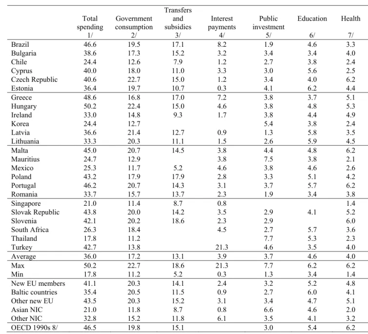
Table 1 illustrates total expenditure and the public expenditure composition across the
sample countries, on an average basis for the period 1999-2003 (or within this period according
to data availability). First, it is striking that the new EU member countries on average report
similar total spending as the “old” EU members and much higher spending than most other
emerging markets. When looking for relatively small governments with spending ratios of less
than 40% of GDP, we only find the Baltic countries belonging to this group. Second, the
divergence in expenditure ratios is enormous ranging from about 18% to 50% of GDP. The
Baltics’ relatively low spending ratio is about one quarter less than that of the central European
countries but it is significantly higher than the average for the Asian emerging economies
Table 1 – Public expenditure in sample countries and country groups, % of GDP Total spending 1/ Government consumption 2/ Transfers and subsidies 3/ Interest payments 4/ Public investment 5/ Education 6/ Health 7/
Brazil 46.6 19.5 17.1 8.2 1.9 4.6 3.3
Bulgaria 38.6 17.3 15.2 3.2 3.4 3.4 4.0
Chile 24.4 12.6 7.9 1.2 2.7 3.8 2.4
Cyprus 40.0 18.0 11.0 3.3 3.0 5.6 2.5
Czech Republic 40.6 22.7 15.0 1.2 3.4 4.0 6.2
Estonia 36.4 19.7 10.7 0.3 4.1 6.2 4.4
Greece 48.6 16.8 17.0 7.2 3.8 3.7 5.1
Hungary 50.2 22.4 15.0 4.6 3.8 4.8 5.3
Ireland 33.0 14.8 9.3 1.7 3.8 4.4 4.9
Korea 24.4 12.7 5.4 3.8 2.4
Latvia 36.6 21.4 12.7 0.9 1.3 5.8 3.5
Lithuania 33.3 20.3 11.1 1.5 2.6 5.9 4.5
Malta 45.0 20.7 14.5 3.8 4.4 4.8 6.2
Mauritius 24.7 12.9 3.8 7.5 3.8 2.1
Mexico 25.3 11.7 5.2 4.6 3.8 4.6 2.6
Poland 43.2 17.9 17.9 2.8 3.3 5.1 4.2
Portugal 46.2 20.7 14.3 3.1 3.7 5.7 6.2
Romania 33.7 15.7 13.7 2.3 1.9 3.4 3.8
Singapore 21.0 11.4 8.7 0.8 1.4
Slovak Republic 43.8 20.0 14.2 3.5 2.9 4.1 5.2
Slovenia 42.1 20.2 18.6 2.3 2.9 6.0
South Africa 26.3 18.4 4.5 2.7 5.7 3.6
Thailand 17.8 11.2 7.7 5.3 2.3
Turkey 42.7 13.8 21.3 4.6 3.5 4.0
Average 36.0 17.2 13.1 3.9 3.7 4.6 4.0
Max 50.2 22.7 18.6 21.3 7.7 6.2 6.2
Min 17.8 11.2 5.2 0.3 1.3 3.4 1.4
New EU members 41.1 20.3 14.1 2.4 3.2 5.2 4.8
Baltic countries 35.4 20.5 11.5 0.9 2.7 6.0 4.1
Other new EU 43.5 20.3 15.2 3.1 3.4 4.7 5.1
Asian NIC 21.0 11.8 8.7 0.8 6.6 4.6 2.0
Other NIC 32.8 15.2 11.8 6.1 3.5 4.1 3.2
OECD 1990s 8/ 46.5 19.8 15.1 3.0 5.4 6.2
1/, 2/, 3/, 4/, 5/ - Average for 1999-2003, source: IMF World Economic Outlook (WEO), and AMECO. 6/ Average for 1998-2001, source: World Bank, WDI 2003.
7/ Average for 1998-2002, source: World Bank, WDI 2003. 8/ Source: Afonso, Schuknecht and Tanzi (2005) for OECD 1990s.
Note: columns 2 through 5 report economic expenditure categories, and that the last two columns report functional expenditure categories.
When looking at the expenditure composition, there are further major differences. But
these differences are much more pronounced for less productive spending categories. Small
government countries tend to spend equally as much, or even significantly more, on productive
spending such as investment and education as the rest of the sample countries. New members
report public consumption around 20% of GDP, twice as much as Asian emerging economies,
GDP while the Asian countries report an average above 6% of GDP. Data on transfers and
subsidies is more sketchy but huge differences are noteworthy: large welfare states of similar
size as in the old EU members predominate in many of the new member countries (with the
Baltics’ featuring somewhat lower expenditure) while such spending in Asian emerging
economies is only fractional. When looking at education, differences across country groups are
much smaller than for total spending. New members, old EU members and other emerging
markets are not far apart from each other. In health, differences are again very significant where
central European countries spend almost 2 and half times as much in % of GDP as the Asian
emerging economies.
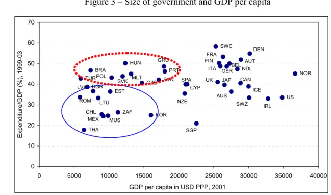
To further improve our picture of the expenditure situation in the sample countries, we
look at per capita GDP as a proxy for the level of economic development and the total
expenditure ratio. Figure 3 provides the evidence. It is interesting to see that the group of poorer
new member states has roughly the same level of per-capital income as most emerging markets.
Korea, the richest new member states and the poorest old EU members (Greece and Portugal)
also report similar per-capita income. Singapore and Ireland would today already fall into the
broader category of industrialised countries after rapid catching up over the past decade.
More relevant for the purpose of this study, however, is to look at expenditure ratios
relative to per-capita income (industrialised country data is included for reference). The stylised
facts confirm that the size of government in the new member countries is much larger than in
some of their emerging market peers and only the Baltics fall into the group of countries with
Figure 3 – Size of government and GDP per capita NZE SPA SGP KOR ZAF MUS CHL MEX THA TUR CYP BGR BRA HUN ROM LVA EST LTU POL
SVK MLT CZE SVN PRT GRC SWE FRA DEN AUT BEL FIN
ITA GER NDL
UK JAP CAN
SWZ ICE AUS IRL NOR US 0 10 20 30 40 50 60 70
0 5000 10000 15000 20000 25000 30000 35000 40000
GDP per capita in USD PPP, 2001
E x penditur e /G D P ( %) , 199 9-03 Source: WDI.
AUS – Australia; AUT – Austria; BEL – Belgium; BGR – Bulgaria; BRA – Brazil; CAN –Canada; CHL – Chile; CYP – Cyprus; CZE – Czech Republic; DEN – Denmark; EST – Estonia; FIN – Finland; FRA – France; GER – Germany; GRC – Greece; HUN – Hungary; ICE – Iceland; IRL – Ireland; ITA – Italy; JAP – Japan; KOR – Korea; LTU – Lithuania; LVA – Latvia; MEX – Mexico; MLT – Malta; MUS – Mauritius; NDL – Netherlands; NOR – Norway; NZE - New Zealand; POL – Poland; PRT –Portugal; ROM – Romania; SGP – Singapore; SPA – Spain; SVK - Slovak Republic; SVN – Slovenia; SWE – Sweden; SWZ – Switzerland; THA – Thailand; TUR – Turkey; UK – United Kingdom; US – United States; ZAF – South Africa.
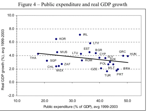
A key question that is frequently asked is whether such large public sectors in the new
member states hurt growth? Alternatively, it has also been asked whether the small public
sectors in several of the emerging markets are detrimental to development if basic services
and safety nets are not provided. This is an empirical question to which there is so far no clear
answer, as illustrated in Figure 4. Per capita growth has been relatively buoyant in recent
years in the small government emerging markets, ranging from two to nine percent per
annum. This shows that low spending is no obstacle to high growth and the prioritisation on
productive spending may also contribute to this picture. Data for the new member states also
suggests that high spending is not necessarily detrimental to growth either. Annual growth
averaged between two and six percent for this country group in recent years. Productive
public spending and other factors such as the boost from impending EU accession may have
Figure 4 – Public expenditure and real GDP growth LTV CYP EST LTU ROM ZA F M EX CHL M US SGP THA KOR IRL P RT CZE M LT B RA
P OL HUN GRC SLV SVK B GR TUR -2.0 0.0 2.0 4.0 6.0 8.0 10.0
10.0 20.0 30.0 40.0 50.0
Public expenditure (% of GDP), avg 1999-2003
R eal G D P gr ow th ( % ), av g 1999-2003
Source: WEO. See country names in Figure 4.
The picture might change slightly when not looking at the best linear fit (which is a
slightly downward sloping line as indicated). The best overall fit would probably be an
inverted U that has its maximum somewhere in the low 30 percent of GDP expenditure range.
Indeed, there is illustrative evidence of a negative relation between rising public expenditure
and economic growth from about this range, as we get a correlation coefficient of -0.56 when
we correlate public spending-to-GDP ratios against real GDP growth for all countries with
public spending above 30 percent of GDP. Though very tentative, this would confirm earlier
presumptions by the authors that optimum spending for growth might be much lower in many
new member and recent emerging market countries.
IV.2. Public sector performance and efficiency via composite indicators
In measuring public sector performance and efficiency, we follow closely the
methodology described above (as developed by Afonso, Schuknecht and Tanzi (2005)). In
summary, our analysis suggests that new EU member countries show an average performance
score that, due to relatively high expenditure, does not suggest very efficient use of public
IV.2.1. Public sector performance (PSP)
As regards public sector performance we have deviated in a few respects from our earlier
study. In the absence of reasonable data on public infrastructure we in particular focus on only
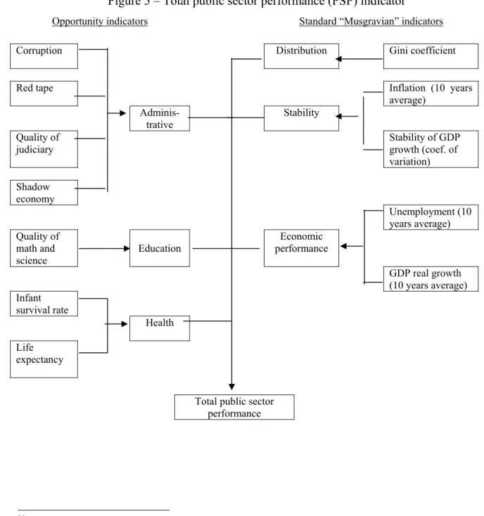
three of the four opportunity indicators and the three respective Musgravian indicators. Figure
5 shows how the sectorial and overall indicators are put together (Annex Tables provide
primary data).14
Figure 5 – Total public sector performance (PSP) indicator
Opportunity indicators Standard “Musgravian” indicators
Corruption Distribution Gini coefficient
Red tape Inflation (10 years
average)
Adminis-trative
Stability
Quality of judiciary
Stability of GDP
growth (coef. of variation)
Shadow economy
Unemployment (10
years average) Quality of
math and science
Education
Economic performance
GDP real growth (10 years average) Infant
survival rate
Health
Life expectancy
Total public sector performance
14
We compile performance indicators from the various indices giving an equal weight
to each of them and the results are reported in Table 2.15 The results for public sector
performance show some interesting patterns, with an overall very diverse picture for the new
EU member states. Starting with the overall PSP indicator, the best performers seem to be
Singapore, Cyprus and Ireland. Other Asian emerging economies and Malta follow this group
of top performers while most new EU member countries and Portugal and Greece post a
broadly average performance. Brazil, Bulgaria and Turkey are placed at the bottom end. The
size of government per se appears to be a too crude instrument of differentiation, when
looking at the score for large public sector countries.
Table 2 – Public Sector Performance (PSP) indicators (2001/2003)
Opportunity Indicators “Musgravian” Indicators Country Adminis-tration Human capital Health Distribu-tion Stability Economic perform. Total public sector performance (equal weights 1/)
Brazil 0.88 0.80 0.96 0.63 0.43 0.77 0.75
Bulgaria 0.80 1.09 0.99 1.17 0.06 0.31 0.74
Chile 1.12 0.86 1.03 0.69 0.92 1.02 0.94
Cyprus 1.12 1.04 1.59 1.54 1.33
Czech Republic 1.00 1.14 1.02 1.19 0.74 0.74 0.97
Estonia 1.25 1.11 0.99 1.00 0.57 0.88 0.97
Greece 0.95 1.04 1.04 1.07 1.67 0.76 1.09
Hungary 1.09 1.16 1.00 1.21 0.97 0.88 1.05
Ireland 1.17 1.11 1.03 1.02 1.64 1.47 1.24
Korea 1.04 1.08 1.01 1.09 1.00 1.60 1.14
Latvia 1.03 0.98 0.98 1.08 0.76 0.88 0.95
Lithuania 0.98 1.12 1.00 1.08 0.37 0.84 0.90
Malta 1.11 1.03 1.04 1.45 1.12 1.15
Mauritius 0.91 0.86 1.00 1.40 1.08 1.05
Mexico 0.80 0.71 1.00 0.75 0.38 1.41 0.84
Poland 0.92 1.08 1.01 1.09 0.83 0.81 0.96
Portugal 1.11 0.88 1.03 0.98 1.30 0.91 1.04
Romania 0.63 1.13 0.98 1.10 0.18 0.63 0.78
Singapore 1.39 1.16 1.05 0.92 2.94 1.71 1.53
Slovak Republic 0.95 1.07 1.01 1.28 1.09 0.77 1.03
Slovenia 1.07 1.13 1.03 1.14 1.35 0.99 1.12
South Africa 1.00 0.66 0.80 0.65 1.23 0.50 0.81
Thailand 1.03 0.99 0.97 0.93 0.94 1.54 1.07
Turkey 0.77 0.75 0.97 0.93 0.17 0.82 0.74
Average 2/ 1.00 1.00 1.00 1.00 1.00 1.00 1.00
Max 1.39 1.16 1.05 1.28 2.94 1.71 1.53
Min 0.63 0.66 0.80 0.63 0.06 0.31 0.74
New EU countries 0.99 1.06 1.00 1.09 0.74 0.86 0.96
Baltics 1.06 1.10 1.02 1.14 0.93 0.95 1.03
Other new EU 0.95 1.05 1.00 1.08 0.66 0.82 0.93
Asian NIC 1.11 1.00 1.00 0.93 1.76 1.44 1.21
Other NIC 0.97 0.91 0.98 0.87 0.96 1.08 0.98
1/ Each sub-indicator contributes 1/6 to total indicator. 2/ Simple averages.
15
When comparing the results for the best performers in this study with those from our
earlier study on industrialised OECD countries, it is noteworthy that Ireland was “only” an
average performer. Portugal and Greece which are near-average in this group were amongst
the weakest in the former study. The results hence show that public sector performance is on
average still somewhat lower in most new EU member countries and emerging markets than
in the “old” industrialised countries but a few of them (notably the new member island
countries and Asian Emerging economies) have broadly caught up.
With regard to sub-indicators, it is interesting to see that the relatively strong
performance of the new EU member states on human capital/education and income
distribution contrasts with a relatively weak one for economic performance and stability.
There is no clear pattern of distinction between Baltics and Central European countries while
the two island countries post strong values for all indicators for which data is available. Asian
Emerging economies performed very strongly on administration, human capital and economic
stability and growth. Overall performance was very equal as regards health indicators.
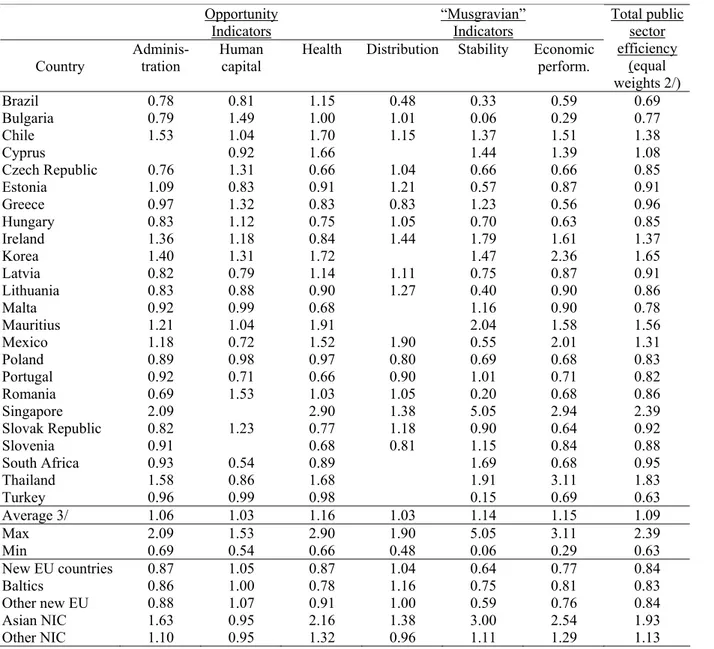
IV.2.2. Public sector efficiency (PSE)
Public sector performance must be set in relation to the inputs used in order to gauge
the efficiency of the state. We compute indicators of Public Sector Efficiency (PSE), taking
into account the expenditure related to each sub-indicator as described in section III.1. PSE
indicators are presented in Table 3 where, due to data limitations for the pre-1998 period in
many countries, averages of the corresponding expenditure item were used for the relatively
Table 3 – Public sector efficiency (PSE) indicators (2001/2003) 1/ Opportunity Indicators “Musgravian” Indicators Country Adminis-tration Human capital
Health Distribution Stability Economic perform. Total public sector efficiency (equal weights 2/)
Brazil 0.78 0.81 1.15 0.48 0.33 0.59 0.69
Bulgaria 0.79 1.49 1.00 1.01 0.06 0.29 0.77
Chile 1.53 1.04 1.70 1.15 1.37 1.51 1.38
Cyprus 0.92 1.66 1.44 1.39 1.08
Czech Republic 0.76 1.31 0.66 1.04 0.66 0.66 0.85
Estonia 1.09 0.83 0.91 1.21 0.57 0.87 0.91
Greece 0.97 1.32 0.83 0.83 1.23 0.56 0.96
Hungary 0.83 1.12 0.75 1.05 0.70 0.63 0.85
Ireland 1.36 1.18 0.84 1.44 1.79 1.61 1.37
Korea 1.40 1.31 1.72 1.47 2.36 1.65
Latvia 0.82 0.79 1.14 1.11 0.75 0.87 0.91
Lithuania 0.83 0.88 0.90 1.27 0.40 0.90 0.86
Malta 0.92 0.99 0.68 1.16 0.90 0.78
Mauritius 1.21 1.04 1.91 2.04 1.58 1.56
Mexico 1.18 0.72 1.52 1.90 0.55 2.01 1.31
Poland 0.89 0.98 0.97 0.80 0.69 0.68 0.83
Portugal 0.92 0.71 0.66 0.90 1.01 0.71 0.82
Romania 0.69 1.53 1.03 1.05 0.20 0.68 0.86
Singapore 2.09 2.90 1.38 5.05 2.94 2.39
Slovak Republic 0.82 1.23 0.77 1.18 0.90 0.64 0.92
Slovenia 0.91 0.68 0.81 1.15 0.84 0.88
South Africa 0.93 0.54 0.89 1.69 0.68 0.95
Thailand 1.58 0.86 1.68 1.91 3.11 1.83
Turkey 0.96 0.99 0.98 0.15 0.69 0.63
Average 3/ 1.06 1.03 1.16 1.03 1.14 1.15 1.09
Max 2.09 1.53 2.90 1.90 5.05 3.11 2.39
Min 0.69 0.54 0.66 0.48 0.06 0.29 0.63
New EU countries 0.87 1.05 0.87 1.04 0.64 0.77 0.84
Baltics 0.86 1.00 0.78 1.16 0.75 0.81 0.83
Other new EU 0.88 1.07 0.91 1.00 0.59 0.76 0.84
Asian NIC 1.63 0.95 2.16 1.38 3.00 2.54 1.93
Other NIC 1.10 0.95 1.32 0.96 1.11 1.29 1.13
1/ These indicators are the expenditure weighted “counterparts” of the indicators of Table 1. 2/ Each sub-indicator contributes equally to the total indicator.
3/ Simple averages.
The results for measuring public sector efficiency show an accentuation of the
findings for public sector performance. This suggests that more public spending often has
relatively low returns as regards improved performance (which is consistent with the findings
of our earlier study for industrialised countries). Most low performers, including most new
EU member states range between 0.8 and 0.9 and Cyprus is the only new member country
with an average PSE score. Countries with a small government sector post a higher PSE score
than the average (and hence even more so than the countries with “big” governments). The
emerging countries of Asia plus Mauritius have most of the highest scores as their good
When looking at sub-indices, the new member states efficiency scores are near
average on human capital and on income distribution. In all other areas, PSE scores are well
below average for the new EU member states. Note also that the income distribution
efficiency score is highest in the countries with smaller welfare states. This confirms findings
elsewhere that welfare programmes in (rich and) poor countries are often poorly targeted and
benefit those with special interests rather than those in need (Alesina (1998) and Schuknecht
and Tanzi (2005)).
All in all the results suggest that efficiency differs enormously across countries. In the
new member states, a relatively average performance (PSP scores) in most countries is
“bought” with too many inputs so that efficiency (PSE) is low. In the next section, we will
analyse whether these findings are confirmed by using a DEA approach.
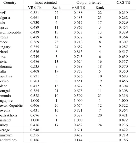
IV.3. Relative efficiency analysis via a DEA approach
We used a DEA approach as described above, using as our output measure the PSP
composite indicator reported in Table 2 and as an input measure the total government
spending as a ratio of GDP. Table 4 presents both the input and the output oriented efficiency
coefficients of the variable returns to scale analysis while the constant returns to scale
coefficients are also reported for completeness.
The results largely confirm the findings of the earlier “macro” approach of
determining efficiency of the public sector. New member states are ranked between 9 and 24
on input scores and between 3 and 18 on output scores, hence reflecting rather diverse and
often below average efficiency. Two countries that also had amongst the top PSE scores are
located on the frontier: Singapore and Thailand. Korea, Chile and Mauritius come next.
Brazil, Greece and Hungary find themselves at the bottom of the list while most new member
states fill the middle ranks. From an input perspective the highest-ranking country uses 1/3 of
the input that the bottom ranking one uses to attain a certain PSP score. The average input
score of 0.55 hints to the possibility that, for the level of output they are attaining, countries
From an output perspective, the top performer achieves twice as much output as the
least efficient country with the same input. The average output score of 0.67 implies that on
average, for the level of input they are using, the countries are only obtaining around 2/3 of
the output they should deliver if they were deemed efficient.
Table 4 – DEA results: one input, one output
Input oriented Output oriented Country
VRS TE Rank VRS TE Rank
CRS TE
Brazil 0.381 22 0.488 22 0.219
Bulgaria 0.461 14 0.483 23 0.262
Chile 0.730 4 0.615 17 0.529
Cyprus 0.489 11 0.867 3 0.454
Czech Republic 0.439 15 0.637 13 0.329
Estonia 0.489 12 0.632 14 0.364
Greece 0.369 23 0.713 8 0.307
Hungary 0.355 24 0.687 9 0.287
Ireland 0.576 8 0.813 4 0.517
Korea 0.749 3 0.743 6 0.639
Latvia 0.486 13 0.624 16 0.357
Lithuania 0.535 9 0.588 18 0.370
Malta 0.408 19 0.753 5 0.350
Mauritius 0.721 5 0.686 10 0.583
Mexico 0.703 6 0.551 19 0.456
Poland 0.412 18 0.627 15 0.304
Portugal 0.385 21 0.678 11 0.308
Romania 0.528 10 0.509 21 0.316
Singapore 1.000 1 1.000 1 1.000
Slovak Republic 0.406 20 0.674 12 0.322
Slovenia 0.431 16 0.731 7 0.364
South Africa 0.676 7 0.529 20 0.421
Thailand 1.000 1 1.000 1 0.822
Turkey 0.416 17 0.482 24 0.236
Average 0.548 0.671 0.422
Minimum 0.355 0.482 0.219
Standard dev. 0.186 0.144 0.186
CRS TE – constant returns to scale technical efficiency. VRS TE – variable returns to scale technical efficiency.
Figure 6 presents the theoretical production possibility frontier associated with the
aforementioned set of DEA results. It shows how far the distance is between the bulk of
countries and the most efficient ones. Nevertheless, there are still very marked differences
between the top, medium and bottom performers inside the production possibility frontier. To
get a clearer picture of differences when abstracting from the best performer we treat