A Facility Layout Planner Tool Based on Genetic Algorithms

A Facility Layout Planner Tool Based on Genetic

Algorithms

Rui Pinto

, Joana Gonc¸alves

, Henrique Lopes Cardoso

, Eug´enio Oliveira

,

Gil Gonc¸alves

and Bruno Carvalho

∗_{SYSTEC - Research Center for Systems and Technologies, Porto, Portugal}

Email: {rpinto, gil}@fe.up.pt

†_{Critical Manufacturing, Moreira da Maia, Portugal}

Email: {jv-goncalves, bacarvalho}@criticalmanufacturing.com

‡_{LIACC - Artificial Intelligence and Computer Science Lab, Porto, Portugal}

Email: {hlc, eco}@fe.up.pt

§_{DEI/FEUP, Faculty of Engineering, University of Porto, Porto, Portugal}

Abstract—Nowadays, in order to maintain their competitive-ness, manufacturing companies must adapt their production methods quickly, with minimum expenditure, to frequent vari-ations on demand. With the shortage of the product life time, flexibility, efficiency and reusability of industrial processes are important factors, which may determine the survival of the company. The ReBORN project is working around these ideas, namely studying how can an old production equipment be re-used into new contexts. The ReBORN Workbench is a simulation tool for factory layout design, which generates solutions based on the production requirements and facilities’ availability, cor-responding Life Cycle Assessment, and associated location cost. This paper is concerned with the ReBORN Workbench module responsible to generate solutions for equipment location, gener-ally know as Facility Layout Problems. A Genetic Algorithm was implemented to solve these problems, which aims to minimize the total material handling costs. The effectiveness of the proposed approach is evaluated with a numerical example and compared with other similar approaches. The results show that the proposed approach is indeed effective to solve problems regarding facilities layout.

I. INTRODUCTION

The ReBORN project [1] – Innovative Reuse of modular knowledge Based devices and technologies for Old, Renewed and New factories – is an ongoing project under the wing of the 7th _{Framework Programme of the European Commission.}

The vision is to demonstrate strategies and technologies that support a new paradigm for re-use of production equipment in old, renewed and new factories, by maximizing the efficiency of this re-usage and making the factory design process straight-forward, shortening ramp-up times and increasing production efficiency and flexibility. This paradigm will give new life to decommissioned production systems and equipment, making it possible to be ‘reborn’ in new production lines. By doing so, production equipment life cycle is extended, contributing to economic and environmental sustainability of production systems, without jeopardizing European machinery industry.

Due to ever decreasing product life cycles and high external pressure to cut costs, the ramp-up of production lines must be significantly shortened and simplified [2]. This is possible

only if the simulated production scenarios mirror accurately the real conditions in terms of speed, performance, costs, availability, reusability and reliability [3]. After the configu-ration and building phases, the ramp-up of new production lines needs adaptation efforts depending on how good the simulated scenarios mirror the real production conditions on site, which is currently not the case. The ability to predict and even forecast the impact of modification within an existing production environment will help during decision making regarding the production methods, effecting effects the overall efficiency of production and influencing main aspects of mass production, such as time, cost and impact. The realization of the ReBORN paradigm for factory layout design and configuration resulted on the implementation of the ReBORN Workbench tool. This simulation tool is meant to help the end-user to configure the system, by aggregating modules for Requirements, Marketplace, System Configurator, System Assessment and Layout Planner.

This paper intends to give a detailed overview of the methodologies used to tackle Facility Layout Planning prob-lems (FLP), which arise from the need to organize facilities in the shop-floor in the most efficient way possible. These methodologies are implemented in the Layout Planner module, which also includes the cmNavigo MES [4]. This manufactur-ing execution system solution is used to display and edit the facilities position in a shop floor layout map, according to the results of the methodologies used. The main goal of a FLP is to minimize total material handling cost inside a facility, which has constrains, such as shop-floor area requirements and location restrictions. This module is able to successfully generate solutions for this type of problems using Genetic Algorithms (GA).

The paper is organized in five more sections. Section II details FLP problems, current approaches and related work. In Section III it is explained in detail the methodology used to formulate and resolve FLP problems, focusing on the implemented GA approach. Section IV depicts all the tests and results obtained, whereas in Section V these results are

discussed. Finally, Section VI concludes the document with final remarks and further steps to be followed.

II. RELATEDWORK

FLP problems are typically related to the location of fa-cilities (e.g., machines, manufacturing cell or department) in the plant area. These NP-Hard problems are known to have a significant impact upon manufacturing costs, work in process, lead times and productivity. The problem’s complexity in-creases exponentially with the number of machinery location. Tompkins et al. [5] stated that a good placement of facilities contributes to the overall efficiency of operations and can reduce up to 50% the total operating expenses. It may be one of the oldest activities performed by industrial engineers and, according to Aleisa & Lin [6], simulation tools are often used to measure the benefits and performance of layouts. Drira et al. [7] explain what are FLP problems, how they are influenced by different shop-floor’s characteristics, and the main approaches used to address it.

A. Problem Formulation

The nature of manufacturing systems greatly influences a FLP problem formulation, because it is very dependent on specific factors and design issues, such as production variety and volume, material handling systems, representation of space, presence of pick-up and drop-off locations, presence of backtracking and bypassing and layout evolution.

According to Dilworth [8], there are four types of layouts according to the production variety and volume: 1) Fixed product layout, where resources move around the product; 2) Process layout, where facilities with similar functions are grouped in different places; 3) Product layout, where facilities are organized in sequence of operations; and 4) Cellular layout, where facilities are grouped into cells to process products with similar characteristics. Regarding the representation of the space available to place the facilities, according to Kim & Kim [9], facilities and space may be regular, regarding shapes and dimensions or they can be irregular [10]. Moreover, horizontal space may be a limitation in some cases, which may originate a need to use a vertical dimension of the shop floor. Kochhar & Heragu [11] referred to these problems as multi-floor layout problems.

There are several material handling systems, such as con-veyors, AGVs, robot or even manual transportation, in order to deliver materials to their destination. Since facility layout impacts the selection of the handling devices and vice-versa, these problems are solved sequentially. According to Yang et al. [12], the layout arrangement types can be: 1) Single row layout, where material flows along a line; 2) Multi-rows layout, where material can flow along several lines; 3) Loop layout, where material flow closes in a ring network; and 4) Open-field layout, where there are no restrictions for material flow. These layout arrangements and material handling systems depend also on the locations for pick-up and drop-off materials, which can be fixed or located at various places, and the presence of backtracking [13] and bypassing [14] on the production

process. Layout evolution refers to the static or dynamic nature of a layout. In a static layout, it is assumed that the production flow will not suffer modifications for a long period of time. The idea of a dynamic layout [15] is to take into account possible changes in the material handling flow over multiple periods.

There are several ways of formulating mathematically a FLP problem, depending on the workshop characteristics and static or dynamic issues. This problem’s formulation is commonly seen as an optimization problem. Most formulations categorize the problem in one of two categories: discrete and continuous formulations. In the case of a discrete formulation, these problems are sometimes addressed as Quadratic Assignment Problems (QAP), where the plant site is divided into equal rectangular blocks and each block is assigned to a facility [16], ensuring that each location is assigned to only one facility. This type of formulation is best suited for dynamic problems. Continuous representation is more relevant when the problem requires to represent the exact position of facilities in the plant site, being more suitable when there are specific constrains, such as orientation of facilities, pick-up and drop-off points or clearance and non overlapping between facilities. These problems are sometimes addressed with Mixed Integer Programming (MIP).

The majority of researchers formulate their problem with one main objective, which is to minimize a function related to the total material handling costs. Some have considered more objectives, which are combined into a single objective by means of the Analytic Hierarchy Process [17] methodology or linear combination of multiple objectives [18]. Others maintain multiple functions for different objectives, using the Pareto approach to generate a set of non-dominated solutions [19]. B. Resolution Approaches

Since they are by nature optimization problems, several approaches exist to address different problem formulations, namely exact methods, such as dynamic programming method and the branch and bound algorithm, and approximated meth-ods, such as heuristics and metaheuristics. Among metaheuris-tics approaches, one can distinguish global search methods, such as Tabu Search [20] and Simulated Annealing [21], evolutionary methods, such as Ant Colony Optimization [22] and the popular GA [23], and a hybridization of different metaheuristics [24].

Jo & Gero [25] explain how GA applied to FLP problems overcome some limitations of conventional design approaches, such as difficulties in problem formulation, generation and evaluation, because of the complexity of the problem, the combinatorial nature of the potential solutions, and the so-phisticated control required. Tate & Smith [26] proposed a GA approach for the QAP that performs better compared with the solutions of the best previously reported heuristics. They conclude that, first, removing solutions from the population is very important for a fast and reliable convergence of the al-gorithm and, second, the combinatorial size of most problems makes it imperative that GA reproduction and mutation only

produce feasible encodings. Chan & Tansri [27] also used a GA approach for the facility layout planning and analyze three crossover operators, namely the Partially Matched Crossover (PMX), Order Crossover (OX) and Cycle Crossover (CX). Mak et al. [28] proposed an approach for GA applied to the facility layout problem, considering various constraints, such as restricted areas, reserved machinery locations and irregularities of the shapes of manufacturing plants. Later, El-Baz [29] compared the effectiveness of his GA solution with Chan & Tansri’s [27] and Mak et al.’s solution [28] and showed that, for the same tests, it performs better. Zouein et al. [30] used GA to solve the site layout problem, characterized by affinity weights and 2D geometric constraints between facilities. Jang et al. [31] applied GA for multi-floor layout problems, considering both horizontal and vertical material handling. Also, Konak et al. [32] used GA for multi-objective layout problems. They considered several objectives, such as minimize cost, maximize performance, maximize reliability, etc.

III. METHODOLOGY

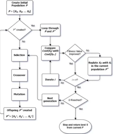
As previously mentioned, our Layout Planner uses a GA implementation to generate optimized solutions for facility layout problems. Since the problems addressed are dynamic by nature, the Layout Planner is prepared only to make discrete representations of the problems (QAP). Also, the Layout Planner is not optimized to formulate properly multi-floor problem, neither irregular shop-floor nor facility shapes. The constraints for the considered problems are: (i) shop-floor area size, (ii) forbidden locations, where no facilities should be placed (doors, pillars, clearances, etc.), (iii) facility size and (iv) material flow between facilities. Fig. 1 represents the flow chart of the implemented GA procedure.

The implemented GA starts with an initial set of random solutions, which constitutes the population. The size of the population P corresponds the number of generated solutions, or also known as chromosomes. Each solution is evaluated according to a predefined fitness function. For QAP, the fitness function corresponds to the total material handling cost func-tion. The chromosomes evolve through successive iterations, known as generations. Each generation is represented by a new population, most of the times different from the previous one. These new populations are not randomly generated. Instead the chromosomes that are part of the current population are selected, merged and modified using genetic operators, such as selection, crossover and mutation, to generate new ones. The new population is known as the offspring. Only the fitter chromosomes are chosen to populate the offspring, by inhibiting the chromosomes that are less fit then the parents to integrate the offspring. For this reason, future generations will always be better then the previous ones. New populations will be generated iteratively until a specific stopping criteria is reached, such as a maximum number of generations G.

Fig. 1. GA Implementation Flow Chart.

A. String Representation

A coding scheme is necessary to represent the problem’s parameters in the chromosome string. For a discrete problem representation, the entire manufacturing plant is divided into N cells and each cell corresponds to a location. These locations are characterized by three parameters, namely the Coordinates, Stateand Equipment. The Coordinates are a pair of values rep-resenting a Cartesian coordinate system point (x,y), specifying this way a unique point location in the shop floor area, which corresponds to the central point of the considered location. The Staterepresents the state of a location, which can be Forbidden (no facility can be placed in that location), Occupied (a facility already was attributed to that location) or Free (the location has no facilities attributed yet). The Equipment represents the facility information, if there is one attributed to the considered position. Facilities are characterized by their identification, name, the type of facility (workstation, servo press, welding module, conveyor, etc.) and their dimensions. Fig. 2 represents an example of the problem parameters and the corresponding encoding into a chromosome string representation.

B. Fitness Function

The fitness function is the objective function of the problem, which in this type of problems corresponds to the total handling material cost of a certain solution, represented by Cost(S) in Equation (1). Each solution corresponds to the location of M facilities in N (≥ M ) positions and is evaluated by calculating its fitness value. Since the goal is to obtain

Fig. 2. GA String Representation.

the solution with maximum fitness, which corresponds to the minimum cost, the fitness function is the inverse of the objective function. Cost(S) = M X i Q(i, S(i)) + M X i M X j [F (i, j) × D(S(i), S(j))] (1)

The total material handling cost of a given solution Cost(S) is defined by two different terms. The fist one represents the sum of all fixed costs Q() in the solution, which corresponds e.g., to the rent of having the facility i in the location S(i). The second term is the sum of all material handling costs between facilities i and j, namely the product between the flow of material F () between facilities i and j, and the distance D() between the position of facilities i and j.

C. Genetic Operators

There are three basic genetic operators used to generate a new population on each generation, namely the Selection, Crossover and Mutation.

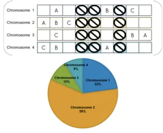
1) Selection: Selection corresponds to the process of sam-pling solutions from the current population. It is represented by a biased selection process, used to determine which solu-tions should be included in the new population. The method used in this implementation was the Biased Roulette Wheel, represented in Fig. 3.

Fig. 3. GA Selection Operator.

The selection criteria of solutions, to integrate the next generation, is based on the fitness value of each solution,

which is converted to a probability of being selected. Fittest solutions have a higher probability of being chosen compared with less fit solutions. The number of well-performed solutions to be replicated into the next generation is represented by the rate of replication R.

2) Crossover: The crossover operator is used to repro-duce the offspring’s chromosomes by crossing two parents chromosomes, as shown in Fig. 4. First, a random position (cutting zone) is selected and aligned on both parents, which divides the parent information to be included in the child. This cutting position should guarantee that at least one Occupied position exists on both parent’s partial information, otherwise the offspring’s may lose facilities in the process and generate invalid solutions. The child is produced by including partial information of both parents, by attributing the State and Equip-ment information to new positions, expect Forbidden ones. This procedure occurs on each generation, with a probability pc.

Fig. 4. GA Crossover Operator.

At this stage, the same facility may be attributed to more than one position. Since duplicated facilities can not occur, a backward replacement is needed. In these cases, one should determine the position of the first occurrence of the duplicated facility in the child, which corresponds to the partial infor-mation of the second parent. This position is used to find a different facility in the first parent. If this new facility already exists in the child, the process is repeated until the chosen facility does not exits in the child. Otherwise, the new facility is included in the child. In case a duplicated facility can not be avoided (no substitute facility is found), then the child is excluded and the parent is included in the offspring.

3) Mutation: The mutation operator is used to introduce randomness to a solution, preventing solutions from being trapped in a local minimum. Fig. 5 represents the mutation procedure.

Since Forbidden positions and facilities information must remain fixed in every generation, the goal of this mutation operator is to swap only the State and Equipment information between two randomly picked positions (except on Forbidden positions) on a chromosome. This procedure occurs on each generation, with a probability pm.

IV. TESTS ANDRESULTS

To evaluate the performance of the implemented GA, a comparative analysis is made using a bench-mark numerical example, taken from Chan & Tansri work [27]. This example was already used to evaluate the performances of GA imple-mentations in the work of Mak et al. [28] and El-Baz [29]. The plant configuration layout is a 3x3 grid. The goal is to place 9 different machines on a layout with 9 positions available. The number of trips between machines is represented on Table I and Table II represent the material handling cost per trip between machines. The flow of materials F () between two machines is calculated by the product between the number of trips and the cost per trip. The fixed cost of this example is assumed to be zero.

TABLE I

FLOW OFMATERIALSBETWEENMACHINES[27].

From/To 2 3 4 5 6 7 8 9 1 100 3 0 6 35 190 14 12 2 - 6 8 109 78 1 1 104 3 - - 0 0 17 100 1 31 4 - - - 100 1 247 178 1 5 - - - - 1 10 2 79 6 - - - 0 1 0 7 - - - 0 0 8 - - - 12 TABLE II

MATERIALSHANDLINGCOSTBETWEENMACHINES[27].

From/To 2 3 4 5 6 7 8 9 1 1 2 3 3 4 2 6 7 2 - 12 4 7 5 8 6 5 3 - - 5 9 1 1 1 1 4 - - - 1 1 1 4 6 5 - - - - 1 1 1 1 6 - - - 1 4 6 7 - - - 7 1 8 - - - 1

Since this example uses 9 machines, there are 365,880 (9!) possible solutions. By applying an exhaustive search to determine the global optimal solution, Mak et al. calculated eight optimal solutions, which correspond to a minimum cost of $4818. The obtained optimal solutions by Mak et al. are shown in Fig. 6.

The performed test consisted on a set of 19 experiments to determine an appropriate combination of the population size P and the stop condition G, which is the maximum number of generations. Besides P and G, the GA implementation uses other input parameters, such as R, pc and pm. In theory,

Fig. 6. Optimal Facility Layout solutions of the bench-mark example [28].

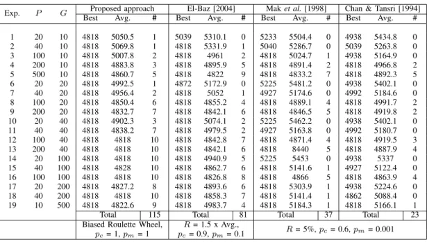
an increase of P and G can produce better solutions, since the number of sampling solutions from the solution space is enlarged. However, the computational effort in searching the space will also increase, which is contradictory to the original objective of using GA. For this reason, Chan & Tansri set the total number of evaluations in each experiment to be less then 3% of the total number of solutions in the solution space (10,886). Table III compares the experimental results of the tests performed between the proposed GA approach, Chan & Tansri [27], Mak et al. [28] and El-Baz [29].

Each of the 19 experiments is run 10 times. The experimen-tal results are expressed in terms of: 1) Best - the toexperimen-tal material handling cost of the best solution among the 10 runs; 2) Avg. - The average of the best material handling costs among the 10 runs; 3) # - The number of runs that obtained one of the eight optimal solution for this problem. Finally, each one of the GA implementations used different input parameters R, pc

and pm, which the authors reported to work well. The results

presented regarding Chan & Tansri’s work are from the PMX operator, since they reported that this operator did provide the best results, compared with OX and CX. Both Chan & Tansri, and Mak et al. used R = 5%, pc = 0.6 and pm = 0.001.

On the other side, El-Baz used pc = 0.9, pm = 0.1 and R

is represented by a 1.5 times the average fitness cut-off limit on each generation. The approach proposed uses pc = 1, pm

= 1 and replication is based on the Biased Roulette Wheel, which revealed better results. Fig. 7 represents GA evolution of one run from the 19 experiments. For viewing purposes, the maximum number of generations shown is 180 instead of 500, since, from all the 19 experiments, the implemented algorithm converged to a solution before reaching the generation number 180.

The test results presented in Table III show that the proposed approach is more efficient than the three other approaches. The proposed approach produces 115 successful runs, which is better compared with the 81 (El-Baz), 37 (Mak et al.) and 23 (Chan & Tansri) successful hits on the other approaches. Also, regarding the total of 10 trials at each experiment of the 19 performed, the current approach succeeded to obtain at least one optimal solution out of ten on every experiment. This was not the case with the other approaches. In fact, by analyzing the average of the total material handling average cost on each experiment, one concludes that the proposed approach performs better, since this value is normally smaller then the

TABLE III

EXPERIMENTALRESULTS OF THE CONSIDERED BENCH-MARK EXAMPLE.

Exp. P G Proposed approach El-Baz [2004] Mak et al. [1998] Chan & Tansri [1994]

Best Avg. # Best Avg. # Best Avg. # Best Avg. #

1 20 10 4818 5050.5 1 5039 5310.1 0 5233 5504.4 0 4938 5434.8 0 2 40 10 4818 5069.8 1 4818 5331.9 1 5040 5286.7 0 5039 5263.8 0 3 100 10 4818 5007.8 2 4818 4961 2 4818 5024.7 1 4938 5164.9 0 4 200 10 4818 4883.8 3 4818 4895.9 5 4818 4891.4 2 4818 4966.8 2 5 500 10 4818 4860.7 5 4818 4822 9 4818 4833.2 7 4818 4892.3 5 6 20 20 4818 4992.5 1 4872 5172.9 0 5225 5481.2 0 4938 5402.1 0 7 40 20 4818 4956.4 2 4818 5052 1 4927 5174.6 0 4992 5184.6 0 8 100 20 4818 4850.4 6 4818 4855.2 4 4818 4889.1 4 4818 4991.7 2 9 200 20 4818 4832.7 7 4818 4842.1 6 4818 4846.5 5 4818 4919.8 2 10 20 40 4818 4902.3 3 4818 5074.1 2 5225 5462.2 0 4938 5402.1 0 11 40 40 4818 4838.2 7 4818 4979.5 2 4927 5163.8 0 4992 5180.7 0 12 100 40 4818 4818 10 4818 4842.8 7 4818 4871.4 4 4818 4919.5 3 13 200 40 4818 4818 10 4818 4842.1 6 4818 8440 5 4818 4887.9 4 14 20 100 4818 4818 10 4818 4940.9 5 5225 5453 0 4938 5337 0 15 40 100 4818 4828 10 4818 4862.7 6 4818 5141.6 1 4927 5122.4 0 16 100 100 4818 4818 10 4818 4826.8 8 4818 4866 5 4818 4863.9 4 17 20 200 4818 4827.2 8 4818 4893.6 6 4818 5303.9 1 4938 5224.6 0 18 40 200 4818 4818 10 4818 4858.3 7 4818 5141.4 1 4862 5088.4 0 19 10 500 4818 4822.6 9 4818 4983.7 4 4818 5184.3 1 4818 5166.1 1

Total 115 Total 81 Total 37 Total 23

Biased Roulette Wheel, pc= 1, pm= 1

R = 1.5 x Avg.,

pc= 0.9, pm= 0.1 R = 5%, pc= 0.6, pm= 0.001

Fig. 7. Proposed Approach Evolution on the 19 Different Experiments.

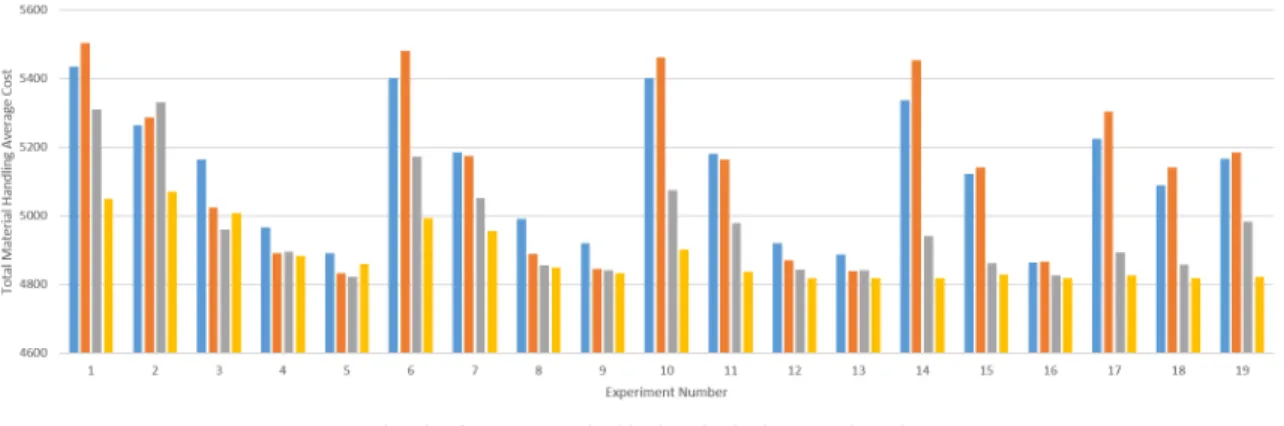
one from the other approaches. In order to analyze and better comparing the four different approaches, Fig. 8 presents in a graphical form the comparison of the total material handling average cost (C()) of each solution on every experiment.

In general, when the P and G increase, C() tends to decrease. All approaches are very sensitive to the variations of P , although both approaches from Chan & Tansri and Mak et al.are a lot more sensitive then the others, since the difference between the C() obtained with a high and low P is significant. Regarding the overall performance off all approaches, despite P and G variations, the C() in practically every experience of the proposed approach is lower then the rest of the approaches (excluding experience 3 and 5).

V. DISCUSSION

Besides the algorithm input parameters, the GA perfor-mance and, consequently, the solution quality are also effected

by genetic operators implemented. Mak et al. pointed out that, in order to ensure fairness, the same input parameters should be used to evaluate the performance of each approach, which is not entirely true. The best parameter values are very problem specific, depending greatly on the nature and implementation of the algorithm. Different approaches require different exploration and exploitation abilities. In the case of GA, the exploration (searching in the solution space) can be adjusted by the pmand the exploitation (concentrating on one

solution) can be adjusted by the pc. Consequently, while the

crossover operator tries to converge to a specific solution, the mutation operator tries to avoid convergence and explore more areas.

According to this, a desirable system behavior is preferable to explore much more in the beginning and, at the end, converge to a optimum solution. This is very difficult to do and, regarding GA, a proper balance between exploration and exploitation should be accomplish. Normally, if pm is too

high, the probability of searching more solutions in the search space increases, however, it prevents population to converge to an optimal solution. On the other side, a pmtoo small may

result on premature convergence, falling to a local optimal solution instead of a global one. Regarding R, this replication rate defines a fitness limit, which is used to select the fittest members of the current population to be included in the new population. These selected members may be modified by crossover and mutation operators, but they can also integrate the new population untouched, mostly on an elitist strategy. By doing so, this strategy guarantees that the best individuals are always present in the next generation.

El-Baz’s approach proved to be better then the one from Mak et al., possibly because of the introduced elitism strategy. On every generation, chromosomes with a cost lower then 1.5

Fig. 8. Total Material Handling Average Cost Comparison.

times the average cost of the entire population are chosen to be included in the next generation. The rest of the chromosomes are deleted. Then, parent chromosomes are randomly chosen from the current population to be transformed, using crossover and mutation operators. The solution from the offspring are generated and included in the new population, stopping when the fixed size of the population is reached.

The proposed approach performs better then El-Baz’s ap-proach, mainly because an improved elitism strategy is im-plemented. Although the number of untouched chromosomes that will be included in the next generation’s population is dynamic (instead of a fixed rate), the proposed approach uses a more selective elitism, a mix of elitism and natural selection. The resulting offspring, regarding the application of the crossover and mutation operators, is carefully evaluated before its chromosomes integrate the new generation’s pop-ulation. Every chromosome of the offspring is compared to the corresponding parents in the previous generation. Only the fittest chromosome between parent and child will integrate the population of the new generation. Before applying again the crossover and mutation operators, the entire new population will be reproduced, using a biased roulette wheel strategy. Since the fittest chromosome of the new population has a bigger probability of being replicated, unfit solutions will also have a bigger probability of being removed.

With this approach, not only the best chromosomes will integrate a new population untouched, but also the same chro-mosomes are chosen as parents for the crossover and mutation operators. On each generation, only the fittest chromosomes are chosen to be part of an elite of champions. This selective elitism works well when both exploration and exploitation rates are very high, since the algorithm can search the full space of solutions and still converge to a optimal solution. This is achieved by performing always crossover and mutation on each chromosome of each generation, using pc = 1 and

pm = 1. Despite the high variety in solutions generated and

based on the analysis of the tests’ results, the conversion to an optimal solution is true, since the elite of champions only includes at least equal or better solution in comparison to

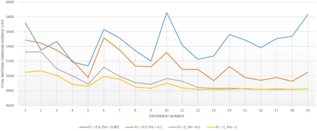
previous ones. In practice, the algorithm generates as most children as possible and, the children are kept only if they are better then the parents. It was verified that the usage of lower pc and pmworsen the algorithms performance. The previous

experiments were repeated with different combinations of the input parameters, represented in Fig. 9.

VI. CONCLUSIONS ANDFUTURE WORK

This paper has presented a GA approach as a methodology to solve discrete representations of FLP problems, which use QAP to formulate the problem. The proposed approach considers several aspects, such as constraints of forbidden positions and the main goal is to minimize the total material handling cost. The effectiveness of the proposed approach has been studied by using the benchmark problem taken from the work of Chan & Tansri [27] and compared with other approaches that used the same benchmark problem, namely Mak et al. [28] and El-Baz [29]. The results have shown that the proposed approach is worthy, because it scored better results to those obtained by others.

Regarding future steps, the proposed approach can be im-proved by extending the scope of FLP problems, considering scenarios of multi-floor layouts, and adapting the formulation to more constraints, such as performance objectives regarding machine task execution. Moreover, a continual formulation of the problem is important to consider constraints such as exact facilities’ position and orientation. The integration of the implemented methodology and the cmNavigo MES needs additional work. Then, current real scenarios would be used to validate the proposed approach, the Layout Planner and the ReBORN Workbench.

ACKNOWLEDGMENT

This research was supported by project ReBORN (FoF.NMP.2013-2) – Innovative Reuse of modular knowledge Based devices and technologies for Old, Renewed and New factories – funded by the European Commission under the Sev-enth Framework Programme for Research and Technological Development.

Fig. 9. Total Material Handling Average Cost of the Current Approach, with Different Input Parameters.

REFERENCES

[1] Steinbeis-Europa-Zentrum. (2016) ReBORN - Innovative Reuse. http://www.reborn-eu-project.org/.

[2] R. Pinto, J. Reis, R. Silva, M. Peschl, and G. Gonc¸alves, “Smart sensing components in advanced manufacturing systems,” International Journal on Advances in Intelligent Systems, vol. 9, no. 1&2, pp. 181–198, 2016. [3] L. Huertas-Quintero, P. Conway, D. Segura-Velandia, and A. West, “A systems integration perspective to manufacturing modelling and simula-tion: An application tool to support electronics manufacturing systems design,” in 2010 IEEE International Systems Conference Proceedings, SysCon 2010, 2010, pp. 415–420.

[4] C. Manufacturing. (2016) cmNavigo MES. http://www.criticalmanufac-turing.com/en/cmnavigo-mes/overview.

[5] J. A. Tompkins, J. A. White, Y. A. Bozer, and J. M. A. Tanchoco, Facilities planning. John Wiley & Sons, 2010.

[6] E. Aleisa and L. Lin, “For effective facilities planning: Layout optimiza-tion then simulaoptimiza-tion, or vice versa?” in Proceedings - Winter Simulaoptimiza-tion Conference, vol. 2005, 2005, pp. 1381–1385.

[7] A. Drira, H. Pierreval, and S. Hajri-Gabouj, “Facility layout problems: A survey,” Annual Reviews in Control, vol. 31, no. 2, pp. 255–267, 2007. [8] J. B. Dilworth, Operations Management-2/E. McGraw-Hill, 1996. [9] J.-G. Kim and Y.-D. Kim, “Layout planning for facilities with fixed

shapes and input and output points,” International Journal of Production Research, vol. 38, no. 18, pp. 4635–4653, 2000.

[10] G.-C. Lee and Y.-D. Kim, “Algorithms for adjusting shapes of depart-ments in block layouts on the grid-based plane,” Omega, vol. 28, no. 1, pp. 111–122, 2000.

[11] J. Kochhar and S. Heragu, “Multi-hope: A tool for multiple floor layout problems,” International Journal of Production Research, vol. 36, no. 12, pp. 3421–3435, 1998.

[12] T. Yang, B. Peters, and M. Tu, “Layout design for flexible manufacturing systems considering single-loop directional flow patterns,” European Journal of Operational Research, vol. 164, no. 2, pp. 440–455, 2005. [13] M. Braglia, “Optimisation of a simulated-annealing-based heuristic for

single row machine layout problem by genetic algorithm,” International Transactions in Operational Research, vol. 3, no. 1, pp. 37–49, 1996. [14] D.-S. Chen, Q. Wang, and H.-C. Chen, “Linear sequencing for machine

layouts by a modified simulated annealing,” International Journal of Production Research, vol. 39, no. 8, pp. 1721–1732, 2001.

[15] G. Meng, S. Heragu, and H. Zijm, “Reconfigurable layout problem,” International Journal of Production Research, vol. 42, no. 22, pp. 4709–4729, 2004.

[16] F. Fruggiero, A. Lambiase, and F. Negri, “Design and optimization of a facility layout problem in virtual environment,” in Proceeding of ICAD, 2006, pp. 13–16.

[17] T. Yang and C. Kuo, “A hierarchical ahp/dea methodology for the facilities layout design problem,” European Journal of Operational Research, vol. 147, no. 1, pp. 128–136, 2003.

[18] C.-W. Chen and D. Sha, “Heuristic approach for solving the multi-objective facility layout problem,” International Journal of Production Research, vol. 43, no. 21, pp. 4493–4507, 2005.

[19] G. Aiello, M. Enea, and G. Galante, “A multi-objective approach to facility layout problem by genetic search algorithm and electre method,” Robotics and Computer-Integrated Manufacturing, vol. 22, no. 5-6, pp. 447–455, 2006.

[20] W.-C. Chiang and P. Kouvelis, “An improved tabu search heuristic for solving facility layout design problems,” International Journal of Production Research, vol. 34, no. 9, pp. 2565–2585, 1996.

[21] L. Chwif, M. Pereira Barretto, and L. Moscato, “A solution to the facility layout problem using simulated annealing,” Computers in Industry, vol. 36, no. 1-2, pp. 125–132, 1998.

[22] M. Solimanpur, P. Vrat, and R. Shankar, “An ant algorithm for the single row layout problem in flexible manufacturing systems,” Computers and Operations Research, vol. 32, no. 3, pp. 583–598, 2005.

[23] H. Pierreval, C. Caux, J. Paris, and F. Viguier, “Evolutionary approaches to the design and organization of manufacturing systems,” Computers and Industrial Engineering, vol. 44, no. 3, pp. 339–364, 2003. [24] J. Balakrishnan, C.-H. Cheng, and K.-F. Wong, “Facopt: A user friendly

facility layout optimization system,” Computers and Operations Re-search, vol. 30, no. 11, pp. 1625–1641, 2003.

[25] J. Jo and J. Gero, “Space layout planning using an evolutionary approach,” Artificial Intelligence in Engineering, vol. 12, no. 3, pp. 149–162, 1998.

[26] D. Tate and A. Smith, “A genetic approach to the quadratic assignment problem,” Computers and Operations Research, vol. 22, no. 1, pp. 73–83, 1995.

[27] K. Chan and H. Tansri, “A study of genetic crossover operations on the facilities layout problem,” Computers and Industrial Engineering, vol. 26, no. 3, pp. 537–550, 1994.

[28] K. Mak, Y. Wong, and F. Chan, “A genetic algorithm for facility layout problems,” Computer Integrated Manufacturing Systems, vol. 11, no. 1-2, pp. 113–127, 1998.

[29] M. El-Baz, “A genetic algorithm for facility layout problems of different manufacturing environments,” Computers and Industrial Engineering, vol. 47, no. 2-3, pp. 233–246, 2004.

[30] P. Zouein, H. Harmanani, and A. Hajar, “Genetic algorithm for solving site layout problem with unequal-size and constrained facilities,” Journal of Computing in Civil Engineering, vol. 16, no. 2, pp. 143–151, 2002. [31] H. Jang, S. Lee, and S. Choi, “Optimization of floor-level construction

material layout using genetic algorithms,” Automation in Construction, vol. 16, no. 4, pp. 531–545, 2007.

[32] A. Konak, D. Coit, and A. Smith, “Multi-objective optimization using genetic algorithms: A tutorial,” Reliability Engineering and System Safety, vol. 91, no. 9, pp. 992–1007, 2006.