A Decision Support System for Online Pricing and Fleet Management in Car Rental Companies

F

E

U

P

A decision support system for online

pricing and fleet management in car

rental companies

José Pedro Silva

Mestrado Integrado em Engenharia Eletrotécnica e de Computadores Supervisor: Beatriz Brito Oliveira

c

Resumo

A indústria de aluguer de automóveis está cada vez mais competitiva e demonstra um crescimento acentuado nos últimos anos, especialmente devido a um crescimento significativo do turismo. Torna-se assim imperativo otimizar cada decisão tomada pela empresa, rentabilizando ao máximo os recursos existentes quer financeiramente, ao fazer o maior lucro possível com cada reserva, quer do ponto de vista ocupacional, reduzindo o número de veículos parados.

Esta tese aborda este problema das empresas de aluguer de carros do ponto de vista tác-ito/operacional, tendo como objetivo apoiar a tomada de decisão diária e recorrente. No entanto, não aborda as decisões estratégicas da empresa, sendo estas vistas como inputs deste problema. É crucial, portanto, que o apoio seja feito de forma online, em tempo real, de forma a contribuir de forma decisiva para que cada decisão tomada seja a melhor com vista aos interesses da empresa.

O objetivo é conceber um modelo matemático que consiga apoiar de forma sustentada esta tomada de decisão em todos os aspetos relevantes à operação da empresa, com especial atenção às questões mais importantes – definição de preços e gestão da frota. Estas decisões devem ser tomadas de forma conjunta para assim maximizar os resultados obtidos pela empresa. Este modelo tem de ter em consideração todas as limitações, como a incerteza da procura, e parâmetros, como o número de estações e grupos de veículos.

Primeiramente, resolveu-se este modelo com recurso a uma resolução offline do mesmo, isto é, resolvendo modelo como um todo, considerando apenas os dados conhecidos no início do hor-izonte temporal. Contudo, um dos principais problemas neste sector é a incerteza na procura e a incapacidade de prever com precisão a procura para períodos de tempo distantes. Assim, depois de desenvolvida esta solução offline, foi desenvolvida uma nova solução para o modelo – online, na qual é utilizada o método de horizonte rolante, abordando o problema por partes e dividindo-o em períodos de tempo mais pequenos. Esta solução consegue assim mitigar este problema na procura, atualizando-a a cada iteração, conseguindo previsões mais realistas.

O modelo concebido, usando os dois métodos de solução, foi testado num ambiente académico tentando reproduzir ao máximo a realidade deste sector, utilizando a informação adquirida na literatura. Os testes feitos visaram validar o modelo e conferir-lhe a capacidade de ser uma mais valia para qualquer empresa deste sector.

Assim, a solução concebida é capaz de apoiar as decisões da empresa em decisões tão rel-evantes como o preço e a gestão de frota, de forma estruturada e factual, utilizando métodos matemáticos rigorosos com vista a melhorar os resultados da empresa e torná-la mais competitiva.

Abstract

The car rental business is increasingly competitive, registering growth in the last years, mainly due to a significant increase of tourism. So, it becomes imperative to optimize every decision made by the company, maximizing the existing resources both from a financial point of view, by making the most profit of every rental, and from an occupational point of view, by raising the occupational rates of the vehicles.

This thesis approaches this problem of the rental companies from a tactical/operational point of view, supporting the daily decision-making yet not approaching the strategical decisions of the company, which are seen as inputs for this problem. It is crucial that the support is made in real time, to make a decisive contribution to the daily decisions regarding the best interests of the company.

The objective is to develop a mathematical programming model that can fully support the decisions in a substantiated way in all relevant aspects to the company operation, especially re-garding the most important questions – price definition and fleet management. These decisions must be made jointly to maximize the company results. This model should take in consideration all the limitations, e.g. uncertainty demand, and parameters, e.g. number of stations and groups of vehicles.

First, the model has been solved using an offline solution, i.e. solving the problem as one, based on the data available at the beginning of the time horizon. However, one of the main prob-lems in this sector is the uncertainty of demand and the inability to predict with accuracy the demand for farther periods of time. So, after this offline solution was proposed, a new solution method – online – was developed, where the Rolling Horizon approach was used, decomposing the problem in parts, dividing it in smaller periods of time. This solution method can mitigate the demand issues, updating it in each iteration, achieving predictions closer to the real values.

The developed model was tested in an academical environment trying to reproduce the busi-ness reality, using the information acquired in the literature. The tests made aim to validate the model and enable it to add value to any company in this business.

The solution method proposed is able to support the decision-making in important aspects as the price definition and fleet management decisions, in a structural and factual way. This is achieved through the use of rigorous mathematical methods, aiming to improve the results of the company and to make it more competitive.

Acknowledgments

First, I would like to thank my Supervisor Beatriz Oliveira all the support and help provided. For being there all the way, providing guidelines and important aids to the final outcome of this thesis. Thanks for all the patience during this time and the immeasurable help in the writing of it. A word also for Professor José Fernando Oliveira for the important help in a few parts of this thesis work. A big thanks to all my family that stood by me all this 5 years. A special thanks to my brother, my mom and my dad for the incredible support. Also to my grandfather and both grandmothers, my godfathers, my aunts and uncles (specially to Batista and Mila) and my cousins that have been a great family support along these years.

Thanks to all my FEUP colleagues, especially to Guilherme Santos, Clésio Silva and João Pereira, that help in this work. For being there when I needed, explaining some doubts and giving me motivation to proceed.

I would like also to thank the great Tripeiros team, João Souto, João Peixoto, José Gabriel and Gonçalo Ribeiro, for providing me incredible moments along this five years. A word also to my teammates from FEUP, UP, Foz, Pedrouços and others that have been important in a personal level.

“Go as far as you can see; when you get there, you will be able to see further”

Contents

2.1.1 Relevance of the Problem . . . 6

2.2 Mathematical Programming Model . . . 8

2.2.1 Variables . . . 9

2.2.2 Objective Function . . . 10

2.2.3 Constraints . . . 11

3 Solution Method: Rolling Horizon Approach 15 3.1 Online Solution Method . . . 16

4 Computational Tests and Discussion 21 4.1 Data and Instance Generation . . . 21

4.2 Offline Tests . . . 24

4.2.1 Initial Tests . . . 24

4.2.2 Upgrades . . . 25

4.2.3 Empty Transfers . . . 26

4.2.4 Empty Transfers and Upgrades . . . 27

4.2.5 Processing Time . . . 28

4.3 Online Tests . . . 29

5 Conclusions 33 5.1 Future Work . . . 33

A Data Tables 35 A.1 Data Table - Offline Tests . . . 35

A.2 Data Table - Online Tests . . . 35

List of Figures

2.1 Stock Definition - General . . . 11

2.2 Stock Definition - Example . . . 12

3.1 The Rolling Horizon Method . . . 17

4.1 Comparison between the offline method with non-updated demand and the online with updated demand, for one type of rental . . . 30

List of Tables

4.1 Initial Tests . . . 24

4.2 Upgrades Tests . . . 25

4.3 Comparison Tests: Upgrades . . . 26

4.4 Empty Transfers Tests . . . 27

4.5 Comparison Tests: Empty Transfers . . . 27

4.6 Upgrades and Empty transfers tests . . . 28

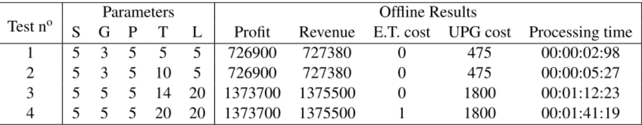
4.7 Demand updated - Offline Results. For comparison between Online and Offline Solutions, see Table4.8 . . . 29

4.8 Demand updated - Online Results. For comparison between Online and Offline Solutions, see Table4.7 . . . 30

4.9 Demand non updated - Offline Results. For comparison between Online and Of-fline Solutions, see Table4.10 . . . 31

4.10 Demand updated - Online Results. For comparison between Online and Offline Solutions, see Table4.9 . . . 31

A.1 Initial Data used in the offline Tests . . . 35

Chapter 1

Literature Review

On this chapter, the literature about the problem that is being approached is reviewed. The most important aspects of the problem analyzed are included in this review: pricing, fleet management, demand forecast and the problem integration, which involves these issues and approaches the problem as one. This study allows for a better understanding of the problem and of the gaps in its state-of-the-art resolution.

1.1

Pricing

Pricing in this business is crucial. Setting the right prices can define the success of the company. Therefore, the challenging decision regarding what price each rental should have has to be well supported and substantiated. This subject is the main issue tackled on several articles such as [1] and [2].

The capacity of understanding price as a powerful tool to revenue management is key. This un-derstanding is growing and there are a few articles exploring this connection in different contexts. This is done on a more general way addressing all important aspects [2] and on a more particular way detailing and addressing specific problems [3,4]. The work done by [2] explains the role of pricing in revenue management and discusses some important tools such as dynamic pricing and price fences that may be useful in practical cases. In [3], the author applies some of these concepts to the hotel business, which is very similar to the car rental industry in this area of pricing. This article applies the dynamic/on-line pricing, which is crucial in these times where the internet and comparison sites that give the best options available are the most used tool to make reservations.

[4] also approaches the hotel business, but in this case the dynamic pricing is a tool to accom-plish better results. Although pricing plays a key role in the revenue management activities of the hotel business, it is not the main goal of this paper. The objective is to maximize profit by deciding how many rooms are sold in advance with lower prices and how many rooms are held to sell with higher prices closer to the reservation date. There is a trade-off between these two decisions. If the hotel chooses to sell more rooms in advance, the outcome may be lower. If the decision is to sell closer to reservation date, it takes the risk of having more rooms un-booked (idle capacity).

2 Literature Review

[1] uses pricing in order to influence demand, applied to the car rental business. In this case, the price is defined considering the future demand and the occupancy of the different stations. The price is higher for reservations that start in a station that has less stock of vehicles and lower for reservations that reallocate vehicles from stations with higher stock to stations with lower stock. The objective is to maintain the stock balance between stations without in the cost of empty transfers. With this method, they reallocate the vehicles by influencing the demand in each station.

1.2

Fleet Management

Fleet management plays a very important role in a car rental company, as the main resources are the fleet of vehicles. Therefore, the management of such resources demands a high focus on these decisions. According to this, several papers (such as [5], [6]) study the impact and techniques to upgrade and optimize these decisions, in order to accomplish better results and profit. Multiple crucial decisions such as fleet size and empty transfers – reallocations – are thoroughly analyzed so that the firm can gain a competitive advantage.

In [5], the author considers some of these important decisions that have to be carefully taken. The fleet size in each time period and in each station has to be previously decided in order to respond to the demand. At the same time, to increase the capacity of response in a station, the decision to perform empty transfers (reallocations) can be taken. Although providing good results, the work is somehow limited and is based on simplifications that may distort part of the reality: it only uses two stations and one type of vehicles.

Paper [6], on the other hand, overcomes these problems and studies a more complex and realistic problem. However, in this case, the rentals are limited to one day of duration.

[7] approaches this problem of fleet management in a general way without particularly ad-dressing the car rental business. In this paper, the objective is assigning the vehicles to the tasks, in the car rental scope – the reservations. The problem includes empty transfers or reallocations of vehicles in order to face demand. Nevertheless, other decisions of fleet management are not fully exploited, since the nature of the case is general and is not applied to any particular business.

1.3

Demand Forecast

One of the main problems of many businesses, not only car rental, is that it is difficult to forecast the future demand. Several works develop methods to solve this problem, yet this remains an open problem in this research field. Therefore, each paper and study attempts to get better results with different techniques and tools.

[8] tackles a problem with only one station and one type of vehicles and consider two types of demand: the demand that is already known, reservations that have been confirmed and scheduled; and the uncertain demand that the firm does not know and tries to forecast.

1.4 Problem Integration 3

In another view of the problem, [4] considers demand as a known parameter, dependent only on the type of reservation and the fixed price for that type of reservation. This case is applied to the hotel business.

The paper [6] faces a similar problem, yet considering uncertain demand, associated with prob-abilities. In this case, the value of the demand is obtained by a probability distribution, dependent on factors such as the type and the price of the reservation.

1.4

Problem Integration

The decisions involved in this business and scope can be divided and are often analyzed separately. Nevertheless, a few works present the advantages of incorporating all or some of the decisions and considering them simultaneously in the decision-making process. Several articles analyze this problem in an integrated way and help the company achieve overall better results.

Paper [1], for example, considers the decision of pricing in each time period, influenced by decisions of fleet management, such as reallocations and variables of demand forecast. This article tries to achieve better results by managing the price in order to reduce the empty transfers yet continuing to respond to the demand. By decreasing the price of a reservation that moves the vehicle to the desired position, the demand for that type of rental increases and the vehicles are moved to preferential locations without costs of empty transfers. One of the gaps of this paper is that it ignores the influence of competitors.

In [3], the author tries to establish the connection between the demand forecast and the pric-ing strategy. In this case, a dynamic pricpric-ing strategy is used with uncertain demand in order to achieve optimal results. This paper also considers capacity control, which includes a few deci-sions regarding fleet management. In this paper, the demand is divided in two different parts: the uncertain demand, the one that is composed by the last-minute reservations; and the demand in advance, which includes the reservations that are made before the start date. The capacity control is applied mainly to the advanced reservations in order to control the number of these low-price reserves. These represent low profits for the company. However, they guarantee booked reserves, translating into certain revenue to the firm. Dynamic pricing is mainly applied to the last-minute reservations in order to maximize profit. In this case, the price is influenced by the occupancy rate. If the rate is low, the price is set lower in order to raise demand. If the rate is high, the price is higher in order to maximize profit, as there is no need for higher demand. The objective is to use these tools in order to maximize profit of the firm. This paper is applied to both the car rental and hotel business.

[9] approaches these problems, although in the airline business. This paper studies revenue management allied with demand information and forecast, and decisions of fleet management such as maintenance and reallocations. In this case, the demand only depends on the type of flight, initial and final destination, and the pricing problem is not tackled. The dynamic scheduling and

4 Literature Review

are the decisions involving fleet management, mainly the ones that influence the schedule of the flights. In this case, the most discussed decision is the maintenance of the aircrafts.

In [10], the problem studied is very similar with the one discussed in this work. Nevertheless, the approach to the problem is more strategical instead of more tactical-operational. The pricing and forecast of demand is not applied in the model, so the main result reflect the fleet management decisions. These two problems are not fully exploited in this paper.

1.5

Conclusion

There are some papers approaching the question of online pricing and fleet management in car rental business. Some of them are very effective and accomplish good results in some of the aspects that are important to this question. However, none of them fully achieves the results needed to effectively support the decisions of the daily needs of a car rental company. There are papers that can support and assist the firm in important areas such as pricing [2,4] or fleet management [7,6] with important results. However, they do not consider the influence of all aspects and decisions involved in this complex and challenging problem. In these cases, the results may have been good but disregarding aspects that are important to the decision-making may hinder a fully supported decision.

Also, a few papers regarding the hotel [4] and airline [9] businesses bring important insights to this problem, since both have similarities in important aspects and decisions that are significant to the car rental business. Nevertheless, some differences hinder the direct application of the results, since they have been developed for another business with a few different requirements.

A few of the works with an integrated solution to this problem accomplish some important results, however they normally simplify the problem, which misrepresents part of the reality. For example, imposing unrealistic limits on the number of stations, the duration of rentals or the lack of some important functionalities such as upgrades. These issues missing in the problem definition do not allow reaching good solutions for car rental.

In other way, a few papers studied the same problem but instead of an operational-tactical approach, they followed a more strategical viewpoint, considering all the decisions of the company for a longer period of time, trying to accomplish the same objective. In [11] the problem definition is essentially the same but the approach involves decisions for long periods (e.g. seasons) such as decisions of buying or leasing vehicles and deciding the size of the fleet. The structure of the solution is similar but due to the changes of the approach to the problem, the decisions of the company are supported in two different “schedules”: a season-based decision support ([11]), and a day by day-based decision support (this thesis).

Concluding, this problem has been studied for some time and there are many papers that accomplish good results and significant improvements to the company involved. Nevertheless, there are relevant particularities that have been disregarded, which do not allow the best support to the extremely important decisions of the company in an increasingly competitive business.

Chapter 2

Problem Definition

The need to increase productivity with the existing resources and become more competitive in the market has become one of the main objectives of the companies, and the car rental business is no exception. To make these companies more competitive every decision has to be well thought and supported with all the relevant information. Decision support systems are powerful tools that give important assistance to the decision making process and can significantly improve the productivity of the company.

In this chapter, the problem will be described in detail, as well as its relevance to this business and all the important aspects and particularities. The problem will also be completely defined in a mathematical programming model, which will be presented and fully explained.

2.1

Problem Description

The problem studied regards the key decisions made in a tactic/operational level of the car rental companies, such as price definition and fleet management. So, in this case, a system is needed that may fully support the firm in all the crucial decisions that have to be made and help maximize the profit, which is the final goal.

The main decision that should to be supported in this scope is the definition of the price of each rental. A rental is characterized by the stations of check-in and check-out, the initial time, the duration of the rental and also the vehicle group requested. The main objective is to define the price for each individual rental considering the existing resources and its demand for each price level. Generally, it is assumed that for higher prices, the demand is lower and for more competitive prices, the demand is higher.

Other important decisions that are key to the company are the ones that involve the fleet man-agement decisions. These include the manman-agement of the assets, the vehicles, and all the necessary adjustments. One important fleet management decision is the reallocation of the vehicles when necessary to achieve better results - empty transfers. In this case, the objective is to respond to the

6 Problem Definition

demand and fully explore the existing resources, obtaining higher profits. Other important deci-sion, with the same objective, is to offer upgrades to the clients when it is not possible to deliver a vehicle of the requested group.

Concluding, the system developed should support the company in these daily-based decisions, in order to help maximize the objective in a substantiated and efficient way. With this approach, the decision making process can be fully supported.

2.1.1 Relevance of the Problem

The car rental industry is increasingly competitive and has shown an accentuated growth in the last years. Therefore, each decision is important and every step should be carefully planned and sup-ported. In this way, the optimization of relevant tactic/operational decisions taken by the company is crucial to achieve the objectives.

Price definition is critical and can define the success, or not, of the company. On the one hand, a higher price can lead to the loss of clients to the competition, and, due to the lack of rentals, lead to holding stock of vehicles, which represent high costs for the company. On the other hand, if the price is too low, it leads to lower margins, lower productivity, and the undervaluation of the assets. The demand levels for different rentals are independent from each other, thus each rental is priced individually. This contributes to make the problem challenging, complex and important, since it increases significantly the number of decisions to be made. In fact, the model has the ability to influence demand by setting the price of some rental, yet this does not affect the demand of a different rental. With this, the model can, for example, deal with a long weekend with high demand and, at the same time, react to the low demand days before that. Nevertheless, the definition of the price of each rental will have some effect in the other rentals, since all the decisions are connected and thus depend on one another. This happens because of the flows of the fleet, as the stocks are influenced by each decision and each rental. For example, a change in price to deal with the high demand of a long weekend will lead to a large stock to be unavailable during those specific days, impacting shorter rentals in that period.

The impact of fleet management decisions on the final profit maximizing objective may not be as relevant as the impact of pricing decisions. However, they have a significant amount of influence in the day-to-day operations of the company and, in an indirect way, on its profit and success. The reallocation of vehicles or the upgrades offered to the clients can highly influence the demand and, with it, the profit of the firm. So, the correct use of these tools – and, especially, their integrated resolution – can define the success of the company and lead in large scale to maximize the objective – the profit.

One of the main difficulties of this business is the uncertainty of demand for the different rentals, especially when analyzing longer periods of time. It is significantly challenging to predict how the market will be in the future, even in few weeks of distance.

Nevertheless, in a shorter period, if pricing and fleet management decisions are closely and frequently adjusted, this difficulty can be mitigated. This uncertain demand is due to the market itself but also to the competitive business, since every change in the competition strategy can

2.1 Problem Description 7

influence and change the future predictions. It thus becomes imperative that decisions are made in shorter frequency, in an on-line fashion, to be able to continuously optimize them, considering the updated predictions every time and to not be as susceptible to the uncertain demand.

In this competitive market, each advantage can be critical to success. The ability to change and to react to the market is important and can help the company to be competitive in every period. With this, the company is less vulnerable to the uncertain demand and can have a fully supported decision regarding the nearby future without compromise in a longer period. Therefore, we aim to develop an optimization method for the pricing and tactical fleet management decisions

8 Problem Definition

2.2

Mathematical Programming Model

In order to fully describe the problem at hand and to support the decision-making processes of the company, a mathematical programming model has been developed considering all the vari-ables of the problem described previously in this chapter. This model supports the decision in a tactical/operational level regarding the daily-based decisions of the company, without involving strategical decisions, such as fleet sizing, which are not addressed and are taken as inputs.

The main decisions of the problem are described as decision variables: • The price for each type of rental;

• The number of rentals fulfilled, for each initial and final station, initial rental time, duration, vehicle group requested and given (due to upgrades, they may be different) and price index (important to make the model linear, yet not to characterize the type of rental);

• The number of empty transfers, for each initial and final station and each group of vehicles; • The stock in each station, for each group of vehicles (auxiliary variable).

These decisions are influenced by the multiple initial parameters that are needed to the correct operation of the model. These parameters are described below and range from technical company inputs, such as the cost of upgrades and empty transfers, to external inputs, such as the demand for each type of rental.

The final objective of the model is to maximize the profit, as the objective function describes. This objective is achieved by the sum of every parcel that influences this goal: the revenue, which results from the fulfilled rentals, the cost of empty transfers and the penalization factor for up-grades.

The model has five essential constraints. These include constraints regarding the stock and its utilization, price discretization, demand as a bound for fulfilled rentals, and limitations on up-grades. The upgrades are controlled by the two group-related indexes in the decision variable of fulfilled rentals. The first one is the group of vehicles that has been given to the customer and the second one is the one that the customer requested. Thus, using a simple two-index binary param-eter to define whether a specific group can be upgraded to other specific group, stock calculation and costs involved needed are easy to obtain and do not need any other decision variable.

The model proposed is a Mixed Integer Linear Program (MIP). Its structure is based on the mathematical programming model proposed in [11] for a strategic approach to the car rental ca-pacity and pricing problem, where e.g. fleeting decisions were made. This is a non-linear math-ematical programming model, with a non-linearity in the objective function, where the decision variables regarding prices and rentals fulfilled are multiplied. Building on this model, yet with an innovative modelling approach that allowed to linearize the objective function and other alter-ations (eg. allowing a more flexible definition of type of rental), we propose the following MIP model for the tactical problem here at hand.

2.2 Mathematical Programming Model 9

This model provides a global view and approach to the problem, considering the totality of the time horizon. Solving this model once, in an “offline” way, does not take into account the changing reality, which is reflected in the existing demand. It gives the full solution for all the periods of time yet it does not regard the uncertain and less reliable predictions to the longer-term demand. With this, the results are more subject to errors and imprecisions. Nevertheless, this model is presented since allows the complete definition of the problem and, later, it will be adapted to an “online” solution method that will be presented and that attempts to overcome this frailty.

2.2.1 Variables Indices:

t= 1, ..., T - Time-unit index;

g= 1, ..., G - Vehicle group index (gp- requested group, gd - given group); s= 1, ..., S - Rental station index ( s1– check-in station , s2– check-out station); p= 1, ..., P - Price index;

l= 1, ..., L - Duration of rental index; Parameters:

Xs1s2g t l p- Rental requests of vehicle from group g , from location s1 to s2, at time t1 with

duration l and price p (demand);

TCs1s2g- Transfer cost of a vehicle from group g , from location s1to s2;

T Ts1s2g- Transfer time of a vehicle from group g , from location s1to s2;

Ns g- Initial stock of fleet per station s , per group g ;

PRIp g- Price value (in monetary units) for a selected price level p and a vehicle of group g ; U PGgpgd - Possibility of upgrading a vehicle from group gp to gd (=1 if it is possible to

upgrade, =0 if it is not);

CU PGgpgd - Cost of upgrading a vehicle from group gpto gd;

M- Big-M large enough coefficient; Decision variables:

ys1s2gpgdt l p - Number of accepted rentals using a vehicle from group gd, which requested a

vehicle of group gp, going from location s1to s2, starting at time t1 with duration l and price level p;

ps1s2g t l p- Price level selected for the rental requesting vehicle group g, going from location

s1to s2, starting at time t1with duration l and price level p; =1 if price has been chosen (= 0 if not) es1s2g t- Number of empty transfers with vehicles from group g, from location s1 to location

s₂at time t; Auxiliary:

10 Problem Definition

2.2.2 Objective Function

Equations2.1represents the objective function of the model, which aims to maximize the profit of the company. This equation incorporates all decisions that influence the economic balance of the company within this scope.

The profit is obtained by subtracting all the costs of operations to the revenue of the rentals. The income comes from the revenue of the rentals, which is the number of rentals times the price charged for that group of vehicles and price index. The cost parcel is composed by the empty transfer costs, which is the number of empty transfers times the transfer cost, and the upgrade costs, which is the cost of upgrade times the rentals where the group requested is different from the group given.

One of the main advantages of the model proposed, which enables its linearization, is the association of the binary decision variable for the selected price with the decision variable for the number of rentals fulfilled through the index of price level in the latter. This allows the objective function to consider the revenue of each rental with no need to multiply two decision variables. The decision variable for the selected price for each type of rental is a binary variable that is equal to 1 for only one price level per each type of rental. In the demand constraint, this limits the number of rentals of each type to the demand associated with the chosen price. The index associated with the price level that is present in the mentioned decision variables and parameters (price decisions, demand levels and rentals fulfilled) is the link between them. It thus allows that the part of the objective function associated with the revenues, which is traditionally the product of number of rentals and the corresponding price, contains only one decision variable, the rentals confirmed, multiplied by the price charged, a previously defined parameter, for each group of vehicles and price level. By doing this, the number of decision variables will increase and consequently the complexity of the model will also intensify. However, this effect is expected to be reduced when compared to the benefit of linearizing the model. That is to say, the advantages of solving a linear model versus a non-linear one are expected to be greater than the disadvantages of adding a new index to a decision variable.

MAXIMIZE Profit = Revenue from rentals - Empty transfer Costs - Upgrade Costs

max P

∑

∑

∑

∑

∑

∑

∑

∑

∑

∑

∑

∑

∑

∑

∑

∑

∑

∑

2.2 Mathematical Programming Model 11

Figure 2.1: Stock Definition - General

2.2.3 Constraints

Capacity constraints: Equations 2.2 represent the correct utilization of the resources in each station so that it does not overcome the stock existing in the same station. The sum of the rentals and empty transfers starting from the station must not exceed the stock existent in the same station, which is applied to any station, period of time and group of vehicles.

S

∑

∑

∑

∑

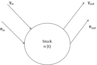
Stock constraints: The equations below,2.3and2.4, are one of the most important elements of the model, since all the decisions made are affected by the existing stock of vehicles.

This represents the sum of all the parcels that involve the entry and exit of vehicles from a station, so the stock of this station can be calculated for the next time period. The stock in a certain station and time period, for a specific vehicle group, is equal to the stock of the previous time period, plus every rental and empty transfer that arrives to the station at that time, minus the rentals and empty transfers that depart from the station in the previous time period.

It should be noticed that the rentals and empty transfers accounted for in the stock calculation of a given period of time are the ones that leave from that station in the previous period of time. However, the ones that arrive and are accounted in this period of time are the rentals that arrive in the same period (Equation2.3). The initial stock is a given input (Equation2.4).

appli-12 Problem Definition

Figure 2.2: Stock Definition - Example

These equations, alongside the previous one, control all the flows of stock and every movement existent in the stations, including the empty transfers and upgrades that may be realized.

ns g t=ns g(t−1) + S

∑

∑

∑

∑

∑

∑

∑

∑

∑

∑

Demand Constraints: Equations2.5control the maximum level of rentals that can be fulfilled by the existing demand. For that, every price level chosen is associated with a demand value. The maximum number in these equations is equal to the existing demand when the corresponding price index is chosen, and it is equal to zero if the index is not chosen. That is to say, the number of rentals allowed is zero if the price has not been chosen and equal to the demand if the price index for that type of rental has been chosen. This is applied to all types of rental.

G

∑

gd=0

2.2 Mathematical Programming Model 13

Price selection Constraints: Equations2.6 control the price level that will be chosen for each rental. This equation limits the number of price levels chosen to one, so that for each type of rental only one price is selected.

P

∑

p=0

ps1s2g t l p= 1 ∀ s1, s2, g,t, l (2.6)

Upgrade Constraints: The following equations limit the existence of upgrades to the ones that are allowed. UPG, an initial data parameter given by the company, defines if a rental that requested a group of vehicles - group requested, could be upgraded to a more valued group of vehicles - group given. If the upgrade is allowed the Boolean parameter is equal to one, if it is not allowed it is equal to zero and it is thus impossible for the model to use that type of upgrades.

S

∑

∑

∑

∑

∑

Domain Constraints: The following constraints define the domain of the decision variables.

ys1s2gpgdt l p∈ Z + 0 ∀ s1, s2, gp, gd,t, l, p ps1s2g t l p∈ {0, 1} ∀ s1, s2, g,t, l, p ns g t∈ Z+₀ ∀ s, g,t (2.8)

Chapter 3

Solution Method: Rolling Horizon

Approach

This chapter will approach the solution method used in the problem discussed. First, the method selected will be presented and described – the Rolling Horizon method. Then, its application to the problem studied will be detailed. Moreover, the adaptations to the previous model, the advantages and disadvantages of this solution method and all its important aspects will be approached.

The method applied to solve this problem was the rolling horizon method. The method is based in a small-scale optimization and provides a faster solution to the problem analyzed. This approach divides the original problem in smaller partitions, based on the time horizon, and solves each sub-problem individually. It allows that, after processing of each sub-sub-problem, the parameters change and the solution method is able to incorporate that and respond to the reality of the problem.

It has been used multiple times in real problems at several industries and it has shown good results and high efficiency.

As an example, [12] applies this method to the energy business. The rolling horizon method is used to reduce the uncertainty in the demand forecast that is witnessed in the energy consumption by the customers. To deal with this uncertainty, the method is applied by analyzing three units of time in each iteration and iteratively solving the model with updated data regarding the demand.

This case has some differences with the problem studied, mainly due to the businesses being very distinct, yet the application of the method is similar. The objective and the way of applying the method are identical in these two cases. The problem that leads to this solution is also the same – to face the uncertain demand forecast.

Other work that applies this method in the presented solution method is [13]. In this case, the method is applied to a different problem that is the control of traffic in a city. [13] uses this method to manage the demand flow in the main streets of a city, to help the signal control in those streets. The method and its application are similar, yet the characteristics of the problem and the objectives are different from the ones here presented.

This method is highly applicable to this business and this problem in particular, since it allows the solution to be determined step by step. This has two main advantages: it allows for the model to

16 Solution Method: Rolling Horizon Approach

be solved faster and it allows for demand levels to be updated, mitigating the problems associated with uncertain forecasting of demand for future horizons.

To apply this method, a new resolution was developed to better respond to the problem de-scribed, based on the model presented in the previous section.

3.1

Online Solution Method

Solving the previously presented model in an offline manner does not allow the update of the demand and other parameters in the middle of the optimization time horizon. To tackle this, an adapted solution method was developed in order to be more flexible and shaped to the alterations that the demand suffers. The demand levels are volatile and difficult to forecast, when analyzing distant periods of time. Solving this model in an online rolling horizon scheme, it will be possible to adapt to changes in this parameter.

To implement this online solution method, it is necessary to create a main function to rule the flow control. This main function will run the model in loop, adjusting the time periods considered, the stock and other updated parameters, and it will retrieve the results of the model in every iteration.

This flow control will allow to update the short-term demand to more accurate forecasts and tackle later time periods afterwards, when the information for them is more accurate. The errors made in the forecasting of the demand are reduced and the support for the decision making can be more substantiated. This is achieved through two parameters related with time: one general index that defines the total number of periods of time in the horizon, and one for the number of periods of time processed in each iteration of the rolling horizon. In each iteration the demand levels for all rental types and prices are updated.

Following the rolling horizon, each iteration solves the mathematical programming model for a part of the time horizon. Each new time period, the model is solved again for a part of the same size, leading to the overlap of some decisions. Therefore, only the decisions made for the first time period of the rolling horizon are fixed. The other decisions will be re-calculated. This allows for the interaction between decision variables of close time periods to be included, yet re-calculated considering new information from the updated demand levels.

The rentals or empty transfers that are fixed in one iteration and impact the following ones are kept in a parameter to be used in later iterations. As mentioned, only the rentals and empty transfers that start before the initial time of the next horizon iteration are kept, the other ones are recalculated in the next iteration.

This overlap of the iterations is a useful tool of this approach since it helps achieve better results by improving part of the model, with better information and less uncertainty. This is better explained in Figure3.1, which shows how the Rolling Horizon method is applied in this case.

The stock for the following time period is calculated in the flow control function. This is equal to the stock from the previous iteration, plus the fulfilled rentals and empty transfers that arrive

3.1 Online Solution Method 17

Figure 3.1: The Rolling Horizon Method

to that station in that period of time, minus the rentals and empty transfers that depart from that station, in that period of time.

The final flow control pseudo-code is presented in Algorithm1. The code starts by initializing the variables that will be used, N (stock) and V (stored reservations for stock purposes), followed by the generation of the model for the first iteration with the initial data values. After that, the cycle for the total amount of iterations starts and the model of the iteration i is solved. Then, if it is not the last iteration, the model keeps the profit of the objective function (OF), only for m = 0, and stores the decisions of rentals that starts in m = 0 (y) in variable V . Then, it calculates the stock for the next iteration, specified in Algorithm2, and generates the next iteration. If the iteration is the last, the profit of all the time periods of the model is accounted. To end the cycle, the variable iis incremented and then the final results are printed.

The calculation of stock is complex and has several aspects to consider, so Algorithm 2

presents this calculation. This Algorithm starts by defining the next iteration stock as equal to the previous one. Then, entries from the current iteration (y) or from past iterations that are stored in V are accounted for each type of rentals and then summed up to the stock variable for the next iteration (N). Afterwords, the variable of rentals kept is updated and the rentals that leave are ac-counted for each type of rental. This is then acac-counted in the stock for the next iteration. Finally, the empty transfers are accounted for each station, summing up the ones arriving in that station

18 Solution Method: Rolling Horizon Approach

Algorithm 1 The flow control code V, N ← 0

i← 0

model(i).generate()

for all i < (Total periods of time - Iteration periods of time + 1) do model(i).solve()

if i < (Total periods of time - Iteration periods of time) then profit ← profit + model(i).OF(m = 0)

V ← y (m = 0)

N(i+1) ← function CalculateStock[N(i),V (in),V (out), e(in), e(out)] model(i + 1).generate()

else

profit ← profit + model(i).OF end if

i= i + 1 end for print Pro f it

3.1 Online Solution Method 19

Algorithm 2 CalculateStock

CalculateStock[N(i),V (in),V (out), e(in), e(out)] {

Vin, In, Out ← 0 for all s, g do N(i + 1) ← N(i) end for for all s, g do for all gp, p, s2do Vin← Vin +V (l = 1) V(l = 1) ← 0 In← In + y(l = 1,t = 0) end for

N(i + 1) ← N(i + 1) +Vin + In Vin← 0 In← 0 end for for all s, g do for all gp, p, s2do for all l do if l > 1 then V(l − 1) ← V (l) + y(l,t = 0) end if

Out= Out + y(t = 0) end for

V(L = max) ← 0 end for

N(i + 1) ← N(i + 1) + Out Out← 0 end for for all s1, s2, g do N(i + 1, s1) ← N(i + 1, s1) − e N(i + 1, s2) ← N(i + 1, s2) + e end for

Chapter 4

Computational Tests and Discussion

This chapter will address the generation of the data that is needed to the correct operation of the model. The computational tests performed will also be approached, regarding the model and so-lution method presented before. An offline resoso-lution of the model will help analyze the structure of the problem. Also, the online solution method will be tested, evaluated and compared with the offline solution method, involving the discussion of these and the analysis of the results obtained. The tests are applied to both solution methods and cover all the relevant subjects from the model studied: upgrades, empty transfers, processing time and stock.

All the tests were performed on an ASUS computer, Intel core i7-7500U CPU 2.70GHz – 2.90GHz, with 8Gb of RAM memory. The optimization solver used was CPLEX and the testes were run in a CPLEX Studio OPL environment.

4.1

Data and Instance Generation

The model presented requires some parameters that will be important to the modelling results and their applicability. These should reflect the business practices of the company and generally are, with the exception of the demand, known and previous defined values, given by the company.

These parameters range from the demand for each type of rental to costs of upgrades and empty transfers. These costs, the stock existent in each station, and the possible values for the prices charged all represent data of which the company is aware and for which already has corresponding values. The unknown parameter, whose definition is based in predictions and forecast, is the demand.

In this application and these specific tests, the data used is not real since this is a scientific experiment with no connection with an actual company. Nevertheless, the goal is to generate data that is similar and applicable to the real business and can, at the same time, be useful to test and validate the model and solution method. These values are expected to approximate the real ones and are tested to confirm their functionality.

22 Computational Tests and Discussion

To dynamically generate new instances (for example, for different number of stations, or ve-hicle groups) without having to manually insert each value, which would take a long time, an instance-generating code was developed in C++, in the Eclipse environment.

The code takes as inputs the size of the sets used in the model (such as number of stations or number of price levels) and the formula to obtain the values of the parameters, and creates the data file needed by the CPLEX Solver to run the model successfully. The code creates the file with the exact structure required by the program, including the minor particularities such as blank spaces and semicolons.

The definition of the demand is an important task of this code. This definition is influenced by many aspects, such as the price value and the periods of time, i.e. how far away is the start of the corresponding rental. In the first tests, Section4.2, since this is a difficult parameter to accurately delimit due to its uncertainty, it was defined as only being dependent on the price value, following the assumption that higher prices lead to lower demand values. However, to better approximate the reality, demand must be influenced by other factors, especially the distance in time to the start of the corresponding rental. The demand for closer periods of time should be higher and more “certain”. On the contrary, the demand for farther periods of time should be lower, since, in a general case, there are less reservations booked and more “uncertain” information of how many more will appear. This approach to the problem may be the most adequate according to the literature and the limitations of this work. The code is ready to implement and easy to adapt to other formulas to define the demand without significant effort.

In the initial stock definition, the value was fixed for all stations and groups of vehicles. Later, this value was systematically changed to accomplish different objectives such as testing the impact upgrades, where the stock of more-valued groups was decreased to zero, and testing the impact of empty transfers, where the stock was set to zero in some stations. In this case, there is no need for complex formulations. However, if necessary, a more complex definition of stock could be implemented based in a formula that depends on the initial station, final station and/or group of vehicles, without significant changes to the data generation code.

The possibility to offer upgrades from one vehicle group to another is represented by a binary parameter that could be settled differently for each pair of vehicle groups. This allows the company to define more independently which upgrades are allowed. In this case, the definition chosen confirms that there only exist upgrades to more-valued groups of vehicles, so that a downgrade is not offered to the customer. The upgrade cost is defined by the company and represents the cost of these upgrades. This cost is not a direct one since there is no operational cost of offering an upgrade to the customer. Nevertheless, this is important to prevent the arbitrary use of this tool. That is to say, to prevent the offer of an upgraded vehicle to have the same influence in the objective function as a normal rental without upgrade. With this, it only uses upgrades if there is no stock of the requested group to fulfill the requests.

The transfer cost and time are also defined in this data file, and these values vary for each combination of initial and final stations. The formula sets higher costs and time duration for longer distances between the stations involved.

4.1 Data and Instance Generation 23

The last data value is the price value defined for each price index and group of vehicles. This can be defined as a formula considering both of these inputs (i.e. PRI = 20 + 10p + 5g). The price defined for each combination depends on the inputs: a higher price index is reflected in a higher price and also a higher group is reflected in a raise of the price.

These values were fixed approximately to real ones. These realistic values have been approx-imated from those found in the literature, which has been studied to know the practices of this sector, especially the use of these parameters (see Chapter1).

The main advantage of this generation procedure is that it is able to create adequate data files to different situations, since it only requires the size of the main sets and, if adequate, the formulas to calculate some values, which is a simple task. With this, this data creating file can be applied to any problem and company with just a few changes.

Creating the data dynamically without taking a significant amount of time is important to the tests described in the next section. The constant changes to the number of stations or vehicle groups, for example, could mean a significant amount of time wasted in the alteration of the data file, yet with this code the time spent changing the data set between tests is significantly lower.

As the two solution methods presented to solve the model require a few changes in the param-eters needed, two distinct data creating files were developed, one for each, yet the content of these files are similar. The online solution method requires two additional parameters, as mentioned in the previous Section (3.1), so its data generating code has a small addition to initialize these parameters. The remaining part of the file is equal in both solution methods.

Algorithm3presents the structure generation code used. Algorithm 3 Data Generation Algorithm

S, G, T, P, L ← Input ofstream my f ile

my f ile.open(”Directory.dat”, std :: ios_base :: out)

for all s1, s2, g,t, l, p do . Demand Parameter Write in my f ile: X [s1, s2, g,t, l, p] ← 10 − p

end for

for all s1, s2, g do . Transfer Cost Parameter Write in my f ile: TC[s1, s2, g] ← 1

end for

for all s1, s2, g do . Transfer Time Parameter Write in my f ile: T T [s1, s2, g] ← 1

end for

for all s1, g do . Stock Parameter

Write in my f ile: N[s1, g] ← 200 − 10 × g end for

for all g, p do . Price Level Parameter

Write in my f ile: PRI[g, p] ← 60 + 20 × p + 5 × g end for

for all g, gpdo . Upgrades Parameter

24 Computational Tests and Discussion

4.2

Offline Tests

These tests were performed to confirm the validity of the model, if there is no problem or error that can affect the final goal. Also, these tests were performed to better understand the structure and behaviour of the model, especially regarding specific issues of the problem (e.g. upgrades).

The tests were performed by solving the model in an offline manner in the first instance, once this makes it easier to test and to analyze the different aspects of the decision making. All the relevant aspects have been approached, especially the ones with a significant influence in the model performance. The discussion of these has also been included. The data used in these tests is presented in TableA.1, in the Appendix.

4.2.1 Initial Tests

After the definition of the model, the initial tests were developed in order to confirm its functional-ity and the absence of errors that could influence the final result. These tests were fundamental to confirm the proper operation of the model, especially the objective function and the most important constraints.

We started by testing small illustrative examples, smaller problems, to be easier to confirm the viability of the model, and then increased the size of the main parameters that impact problem size until reaching an approximation to the realistic values. These main parameters – periods of time, stations, price levels and also groups of vehicles – influence the size of the problem in terms of decision variables and constraints, increasing significantly the complexity of the problem.

In these tests, neither upgrades nor empty transfers are used. They will be explored in the following sections (4.2.2,4.2.3and4.2.4).

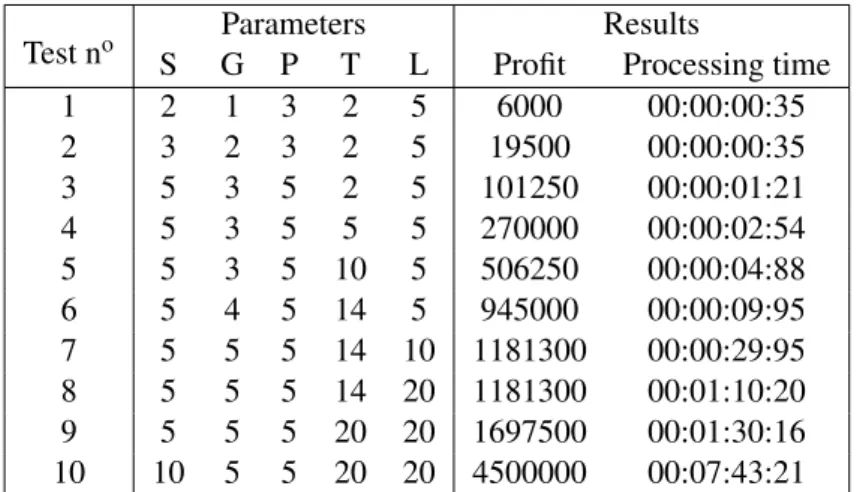
These tests are shown in Table4.1, including the parameters used and the results for each test, using the nomenclature presented in Section2.2.

In Table4.1, and in all tables throughout this document, for the sake of simplicity, "Processing time" is presented in the format hh:mm:ss:ms, where hh stands for hours, mm for minutes, ss for seconds and ms for milliseconds.

Table 4.1: Initial Tests

Test no _S Parameters_{G P T L Profit} Results_{Processing time}

1 2 1 3 2 5 6000 00:00:00:35 2 3 2 3 2 5 19500 00:00:00:35 3 5 3 5 2 5 101250 00:00:01:21 4 5 3 5 5 5 270000 00:00:02:54 5 5 3 5 10 5 506250 00:00:04:88 6 5 4 5 14 5 945000 00:00:09:95 7 5 5 5 14 10 1181300 00:00:29:95 8 5 5 5 14 20 1181300 00:01:10:20 9 5 5 5 20 20 1697500 00:01:30:16 10 10 5 5 20 20 4500000 00:07:43:21

4.2 Offline Tests 25

These results show that the processing time grows with the increase of parameters and, re-spectively, the number of decision variables. Especially with the increase of stations to 10, the processing time grows to 7 minutes, which represents a raise of 500% comparing with the previ-ous time, where the number of stations was 5. This shows the influence that these parameters have in the processing time.

Another result is the raise of the profit when the number of parameters increase, especially the number of stations, groups and periods of time. This is an expected result since increasing these values increases the existing stock (the stock is defined as constant throughout all the stations and groups) and, also consequently, the number of fulfilled rentals increase.

4.2.2 Upgrades

In order to analyze the aspects relevant to the upgrading operation, the initial data, used as input to the model, was changed. The stock and other parameters were manipulated to encourage the existence of upgrades to be analyzed afterwards.

The first adaptation to ensure that the model would provide upgrades in the optimal solution was setting the cost of upgrades significantly lower comparing to the price charged for the rentals. This aims to reduce the negative impact of offering upgrades in the objective function, the final profit of the company. Moreover, the possibility of offering every combination of upgrade was set, so that all the groups of vehicles could be upgraded to a more-valued group.

The stock of vehicles was set null to all the groups of vehicles, except the first two. The stock of these first two was set to be high in order to fulfill the existing demand for this group and still have excess stock to be an upgrade option to the other groups that did not have stock. With this, the model is influenced to perform upgrades in the final solution.

As for the parameter that controls which groups may be upgraded to which groups, it was defined that the upgrades could happen in every allowed combination of groups. Despite some of these adaptations being redundant, they were applied to ensure the presence of upgrades in the final solutions.

In these tests, the cost of empty transfers is set to a high value, so as to influence the model to not use this tool. Those are analyzed separately in the sub-section4.2.3and including both tools in the sub-section4.2.4.

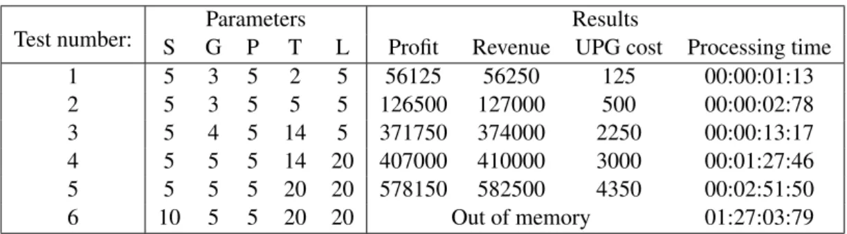
Table 4.2: Upgrades Tests

Test number: _S Parameters_{G P T L Profit Revenue} Results_{UPG cost Processing time}

1 5 3 5 2 5 56125 56250 125 00:00:01:13

2 5 3 5 5 5 126500 127000 500 00:00:02:78

3 5 4 5 14 5 371750 374000 2250 00:00:13:17 4 5 5 5 14 20 407000 410000 3000 00:01:27:46 5 5 5 5 20 20 578150 582500 4350 00:02:51:50

26 Computational Tests and Discussion

Table4.2represents the tests performed to the model with the offline solution involving up-grades. These results reflect the influence of the upgrades in the model and its processing time. With the increase of the parameters to high numbers, especially the increase of the stations to 10, the model, after almost one and a half hours of processing, reached the maximum memory of the system and could not complete the solving procedure, reaching the breaking point.

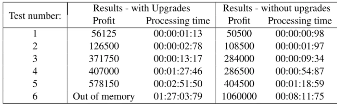
Table4.3shows the comparison between the solutions involving and not involving upgrades for the same problem, including parameters and data used. As mentioned before, the only differ-ence consists in the possibility of offering upgrades. These tests reveal that the possibility to offer upgrades increases significantly the processing time, keeping constant the remaining parameters and initial data. The comparison shows that upgrades increase the complexity of the problem, raising significantly the processing time, especially with high number of parameters involved. Nevertheless, the profit with upgrades is significantly higher, since the possibility of providing upgrades increases the capacity to respond to the demand, using more-valued groups when the stock of the requested group is not enough. The difference of profits between the solution with and without upgrades is considerably higher, reaching 40% of increase, when the parameters used are large. This evidences the importance of upgrades in this problem.

Table 4.3: Comparison Tests: Upgrades

Test number: _ProfitResults - with Upgrades_{Processing time} Results - without upgrades_{Profit Processing time} 1 56125 00:00:01:13 50500 00:00:00:98 2 126500 00:00:02:78 108500 00:00:01:97 3 371750 00:00:13:17 284000 00:00:09:34 4 407000 00:01:27:46 286500 00:00:54:87 5 578150 00:02:51:50 404500 00:01:18:59 6 Out of memory 01:27:03:79 1060000 00:08:11:75 4.2.3 Empty Transfers

Following the upgrade tests, the empty transfers were analyzed to confirm the applicability of this tool. The initial data was changed to verify this and to influence the model to favour the use of empty transfers.

The same procedure applied in the upgrade tests was used. The cost of empty transfers was set to a low value to induce the use of this tool and the transfer time was set to one time unit, the minimum possible, to assist in the objective. The stock of vehicles was changed to zero in all the stations except the first two, where it was set to a high value. This, alongside the low demand existent in all the stations, confirms that the best scenario is the use of the empty transfers to reallocate vehicles to meet demand from the stations that have excess of stock, to the stations that are lacking.

As occurred with the upgrades, this objective could be verified without resorting to such changes, however, these adaptations in the data can help reaching the objective of this tests.

4.2 Offline Tests 27

Table 4.4 shows the results of the main tests performed involving empty transfers, without considering the possibility to upgrade.

Table 4.4: Empty Transfers Tests

Test number: _{S G}Parameters_{P T L Profit Revenue} Results_{E.T. cost Processing time}

1 5 3 5 5 5 81984 82050 66 00:00:02:27

2 5 4 5 14 5 316310 316400 88 00:00:09:85 3 5 5 5 14 20 395390 395500 110 00:01:05:66 4 5 5 5 20 20 567890 568000 110 00:02:07:89 As seen in Table4.4, inducing the use of empty transfers does not affect significantly the pro-cessing time, as the upgrades do. This may be result of this adaptation not changing the structure of the problem, unlike upgrades. In this situation, if there are no upgrades, the problem is separa-ble in sub-prosepara-blems for each group of vehicles, while in the case of empty transfers, the absence of these movements does not allow that the problem is solved in sub-problems since the stations and corresponding stocks continue to be dependent on each other.

Table 5.5 compares the previous tests performed using empty transfers with tests with the same initial data and the same parameters, yet not using empty transfers.

Table 4.5: Comparison Tests: Empty Transfers

Test number: Results with Empty transfers_{Profit Processing time} Results without Empty transfers_{Profit Processing time} 1 81984 00:00:02:27 80970 00:00:02:20 2 316310 00:00:09:85 313320 00:00:09:88 3 395390 00:01:05:66 391650 00:01:05:18 4 567890 00:02:07:89 564150 00:02:04:57

As shown in Table4.5, the empty transfers have a small effect in both the objective function, the profit, and the processing time, which is nearly the same with and without empty transfers.

Although the small influence in these parameters, the results show an increased profit with the empty transfers involved. This is evidence of the importance of empty transfers, which is not the same as upgrades, yet provides the company with better results. This is even more important in a competitive market as the rental business is, where every tool that allows companies to better meet demand is useful and should be applied.

4.2.4 Empty Transfers and Upgrades

In reality, both empty transfers and upgrades are used simultaneously and, in the final objective function value, parcels related with both tools appear. To validate the simultaneous use of these tools, the following tests were performed.

28 Computational Tests and Discussion

assigned with stock, with the rest having null stock. Also, both of the costs (empty transfers and upgrades costs) were set to a low value to assist in this objective.

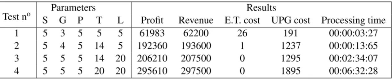
Table 4.6: Upgrades and Empty transfers tests

Test no _SParameters_{G P T L Profit Revenue E.T. cost}Results_{UPG cost Processing time}

1 5 3 5 5 5 61983 62200 26 191 00:00:03:27

2 5 4 5 14 5 192360 193600 1 1237 00:00:13:65 3 5 5 5 14 20 206210 207500 0 1295 00:02:34:07 4 5 5 5 20 20 295610 297500 0 1895 00:06:32:28 The results of these tests are represented in Table4.6. As observed in the table, the number of empty transfers used decreases with the raise of the parameters. This could mean that all the stock is used to fulfill the demand in current stations and there is no excess to use for empty transfers. The existing stock responds to the demand for that station, for all possible groups (considering upgrades), and there is no stock left to use to perform empty transfers. This may occur since the profit from rentals (both regular and upgrades) is higher than the one possibly associated with the rentals that would be allowed by the occurrence of the empty transfers (for which there is no immediate profit associated, only being reflected in the following periods of time).

4.2.5 Processing Time

The processing time is the reflection of how the model is working. That is to say, if there are less decision variables, the model will be smaller and therefore faster to solve, with low processing time. In opposition, with more decision variables involved, the results are more difficult to obtain, thus the model will be slower to solve, with higher processing time and requiring more processing power.

The solution of this problem is supposed to support the company in a daily basis. Therefore, if the processing time is not realistic, i.e. not fast enough, it cannot be applied in the company. So, as a tactical/operational level decision support, this solution must have a faster processing time, even with instances sizes that approximates the reality, in order to be run multiple times.

An important factor that directly influences the processing time is the existence of upgrades, as discussed before. If there are no upgrades, each group of vehicles could be dealt with separately, so the number of decisions and the processing time would be significantly less. This aspect is fully described in the previous Upgrades tests section (4.2.2).

The size of parameters is another important factor to the processing time. The number of stations, groups, price levels and periods of time have a direct impact in the processing time. The amount of these is connected with the number of decision variables: their increase will raise the number of decision variables and, consequently, the processing time of the resolution. This factor is demonstrated in a few tests, especially in Table 4.1 where, without considering upgrades or empty transfers, the results for the processing time reflect the the size of the corresponding sets of parameters.