BJRS
RADIATION SCIENCES
07-02A (2019) 01-14ISSN: 2319-0612
Accept Submission 2018-10-31
Validity studies among hierarchical methods of cluster
analysis using cophenetic correlation coefficient
P. R. Carvalho
a; C. S. Munita
a; A. L. Lapolli
a aInstituto de Pesquisas Energéticas e Nucleares (IPEN - CNEN/SP)Av. Professor Lineu Prestes 2242, 05508-000 São Paulo, SP, Brazil
prii.ramos@usp.br
ABSTRACT
The literature presents many methods to produce data set clusters and the better method choice becomes hardest because the various combinations between them based on different dissimilarity measures can lead to different cluster patterns and false interpretations. Nevertheless, little effort has been expended in evaluating these methods empirically using an archeological data set. In this way, this work has the objective to develop a comparative study of the cluster analysis methods and to identify what is the most appropriate for an archeological data set. For this, 45 ceramic fragments samples data set was analyzed by instrumental neutron activation analysis (INAA). And, five hierarchical methods of cluster were used to this data set: Single linkage, Complete linkage, Average linkage, Centroid and Ward. The validation was done calculating cophenetic correlation coefficient values by a statistical program R and the comparison between them showed the average linkage method was more accurate for the 45 ceramic fragments samples data set. With this, the statistical program R showed be an tool option for other scientists to calculate their cophenetic correlation coefficient and to identify the more accurate methods for their archeological data set.
1. INTRODUCTION
In the last years, cluster analysis has increasing your emphasis in multivariate data analysis. However, clustering techniques are tools where the application and interpretation are subjective, depending on the experience and user perspicacity [1]. Different clustering methods produce different results when applied to the same data [2]. Nevertheless, little effort has been expended in evaluating these methods empirically using an archaeological data set.
In archaeological studies several analytical techniques are used to study the chemical and mineralogical composition of many archaeological materials with the objective of to find yours origin, generating a large data set. Thus, the multivariate statistical methods become indispensable for the results interpretation.
These multivariate techniques, unsupervised and supervised, are accompanied by modern computational programs, which provide visualization and interpretation. Several methods have been used, as cluster analysis, discriminant analysis, principal component analysis, among others. However, the one is cluster analysis [3]. The cluster analysis purpose is to bracket the samples based on similarity or dissimilarity [4]. The groups are determined in order to obtain homogeneity within the groups and heterogeneity between them [5].
The literature presents many methods to produce data set clusters[2, 5, 6, 7, 8] and the most accurate method choice becomes hardest, because the combinations various between them based on different dissimilarity measures can lead to different cluster patterns and false interpretations. [2].
In this way, the objective of this work is to development a comparative study for cluster analysis methods and to identify what is the most accurate for archaeological data set.
This study was accomplished using the an Archaeometric Studies Group data set from IPEN-CNEN/SP, where there are 45 ceramic fragments samples analyzed by instrumental neutron activation analysis (INAA). The methods used to identify what is the most accurate for Archaeometric Studies Group data set were: Single Linkage, Complete Linkage, Average Linkage, Centroid and Ward. The validation was done calculating the cophenetic correlation coefficient values to analyze the grouping generated quality by the hierarchical methods of cluster analysis, as also to determine a criterion for evaluate the various grouping techniques efficiency [9].
In addition, considering the existence of several statistical programs and programs complexity, a statistical program R script with some functions was created to obtain the cophenetic correlation coefficient values.
2. MATERIALS AND METHODS
2.1 Data set
This study was accomplished using a data set of the Archaeometric Studies Group from IPEN-CNEN/SP, there are 45 ceramic fragment samples from three archaeological sites:
A. Prado site: located at Engenho Velho Farm, in Perdizes city, State of Minas Gerais, Brazil, 19º14´25´´ LS–47º16´00´´ LW;
B. Água Limpa site: located in the confluence of three small farms, in Monte Alto city in the North of São Paulo State, 21º15´40´´ S–48º29´47´´ W;
C. Rezende site: located in Paiolão farm, in Piedade, Paranaíba Valley, 7 km from Centralina city, Minas Gerais State, Brazil, 18º33´ LS, 49º13´ LW;
They were analyzed by Instrumental Neutron Activation Analysis (INAA) to determine the mass fractions of 13 chemical elements: As, Ce, Cr, Eu, Fe, Hf, La, Na, Nd, Sc, Sm, Th and U. The details on the sample preparation and the analytical method were published in another work [10].
2.2 Cluster Analysis
Cluster analysis is a statistical interdependence technique whose primary purpose is to group the samples based on similarity or dissimilarity [4] from predetermined variables. The groups are formed so that each sample is similar to the others in the grouping, thus seeking to minimize the variance within the group and to maximize the variance between the groups, that is, to maximize the homogeneity within the groups and the heterogeneity among them [5]. Thus, if the classification is successful, the objects within the groupings will be close together when represented graphically and different groupings will be distant.
For this, the samples are initially treated individually and then analyzed in a correlation matrix, or similarity/dissimilarity samples matrix, where sample-sample, sample-group and
group-group distances are calculated successively, until a single group-group formation. In general, the smaller distance between the samples, they have the greater similarities.
Thus, it can be said that the clustering process basically involves two stages: the first relates to the estimation of a similarity measure (or dissimilarity) between the sample units; and the second, with the adoption of a grouping technique for group formation.
The distances are dissimilarity measures used for data set with quantitative variables. A large dissimilarity measures number have been proposed and used in cluster analysis [2, 7]. Among these distances, the chosen were: Euclidean, Squared Euclidean, Manhattan (or City-Block) and Mahalanobis. Once the metric is chosen, the second step is to choose which clustering algorithm will be used to form the groups.
In the literature, several cluster methods are found [2, 5, 6, 7, 8], and the researcher has to decide that is most accurate for its purpose. Most methods can be classified into two large families of methods: hierarchical and non-hierarchical. In this work, will be studied the hierarchical agglomerative methods (Single Linkage, Complete Linkage, Average Linkage, Centroid and Ward).
2.2.1 Single linkage method
The Single linkage method is between the oldest methods, developed, initially, by polish researchers in the 1950s [11]. It was first described by Florek et al. [12] and later by Sneath [13] and Johnson [14]. The distance between two cluster (C1) and (C2∪ C3) is defined as the minimum distance between any sample in a cluster and any another sample [8] and can be obtained by:
d(C1, C2∪ C3) = min {d(C1, C2), (C1, C3)} (1)
This method tends to produce unbalanced and straggly clusters (“chaining”), especially in large data sets. Does not take account of cluster structure [8].
2.2.2 Complete linkage method
The Complete linkage method is similar to the Single linkage method except in the distance between two clusters (C1) and (C2∪ C3). It is now defined as the largest distance between samples pairs in each cluster, rather than the smallest [15] and can be obtained by:
d(C1, C2∪ C3) = max {d(C1, C2), (C1, C3)} (2)
This method Tends to find compact clusters with equal diameters (maximum distance between objects). Does not take account of cluster structure [8].
2.2.3 Average linkage method
In Average linkage – also known as the unweighted pair-group method using the average approach (UPGMA) – the distance between two clusters is the average of the distance between all pairs of samples that are made up of one sample from each group [8]. The distance between clusters is determined by the Lance-William correlation:
d(C1, C2∪ C3) =
n2. d(C1, C2) + n3. d(C1, C3)
n2+ n3 (3)
where n2 and n3 are the number of samples in clusters C2 and C3, respectively [4, 11].
This method tends to join clusters with small variances. Intermediate between single and complete linkage. Takes account of cluster structure. Relatively robust [8].
2.2.4 Centroid’s method
In Centroid’s method the dissimilarity of two clusters is expressed as the distance of centroids of these clusters. Each cluster is represented by the its samples average, which is called the centroid. The distance between clusters is determined by the Lance-William correlation:
d(C1, C2∪ C3) = n2 n2+ n3 d(C1, C2) + n3 n2+ n3 d(C1, C3) − n2n3 (n2+ n3)2 d(C2, C3) (4)
where n2 and n3 are the number of samples in clusters C2 and C3 [4, 11].
This method assumes points can be represented in Euclidean space (for geometrical interpretation). The more numerous of the two groups clustered dominates the merged cluster. Subject to reversals [8].
2.2.5 Ward’s method
Ward’s method was proposed by Ward in 1963 [16] and is also called "Minimum Variance” [2]. In this method, the two clusters fusion is based on the size of an error sum-of-squares criterion [8], in order to maximize the groups internal homogeneity [4]. The distance between clusters is determined by the Lance-William correlation:
d(C1, C2∪ C3) = n1+ n2 n1+ n2+ n3 d(C1, C2) + n1+ n3 n1+ n2+ n3 d(C1, C3) − n1 n1+ n2+ n3 d(C2, C3) (5)
where n1, n2 and n3 are the number of samples in clusters C1, C2 and C3 [4, 11].
This method assumes points can be represented in Euclidean space for geometrical interpretation. Tends to find same-size, spherical clusters. Sensitive to outliers [8].
2.3 Cophenetic Correlation Coefficient
After applying the method chosen for the groups formation the cophenetic correlation coefficient (CCC) has been used to verify the cluster quality. Since its introduction by Sokal and Rohlf [17], the CCC (Eq. 6) has been widely used in studies, both as a fit degree measure of a data set classification and as a criterion for evaluating the various clustering techniques efficiency [9].
CCC = ∑ ∑ (cik− c̅) n k=i+1 n−1 i=1 (dik− d̅) √∑n−1i=1 ∑nk=i+1(cik− c̅)2√∑ ∑ (dik− d̅) 2 n k=i+1 n−1 i=1 (6) Where:
cik = dissimilarity value between samples i and k, obtained from the cophenetic matrix;
dik = dissimilarity value between samples i and k, obtained from the dissimilarity matrix.
c̅ = 2 n(n − 1) ∑ ∑ cik n k=i+1 n−1 i=1 (7)
The cophenetic correlation coefficient consists in comparing the observed distances between the samples and the distances predicted from a clustering process [6], by measuring the fit degree between the original dissimilarity matrix and the resulting matrix from the simplification provided by the clustering method.
In this work, the cophenetic correlation coefficient was used to validate the methods and to find the most accurate for the data set.
2.4 Script
The statistical study was performed using the statistical program R. The R is a programming environment with an integrated set of software tools for data manipulation, calculations and graphical presentation [18]. The structure is a public and free open source which has been widely
d̅ = 2 n(n − 1) ∑ ∑ dik n k=i+1 n−1 i=1 (8)
accepted by researchers around the world. However, by using programming language, the R, requires the user a brief programming knowledge.
In this way, a script with functions of the statistical program R was developed to calculate and to identify the cophenetic correlation coefficient of the cluster analysis hierarchical method more accurate for a data set. This guide purpose is to facilitate the study of researchers who are not from the statistical area or are not familiar with the program.
The more important functions used in this script were:
• vegdist used to calculate the Euclidean, Squared Euclidean, Manhattan and Mahalanobis distances;
• hclust used to apply the cluster methods;
• cophenetic used to calculate the cophenetic correlation coefficient.
3. RESULTS AND DISCUSSION
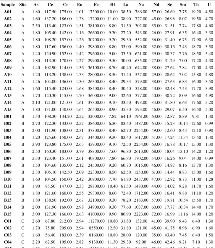
The study was made using a 45 ceramic fragment samples data set which were determined As, Ce, Cr, Eu, Fe, Hf, La, Na, Nd, Sc, Sm, Th, and U by INAA. Where, their mass fractions values are in the Table 1.
Initially, the results were transformed to log10. This transformation before applying
multivariate statistical techniques is a usual procedure in archaeometric studies and there are two reasons for this: the first is explained by the fact that a normal logarithmical distribution of the elements exists. The other is the difference magnitude between elements, which it was found in percentage and trace level [19].
Then, the detection of the outliers was done by means of Mahalanobis distance using the lambda Wilks criterion as critical value [20]. In this outlier detection method, when the calculated value for the Mahalanobis distance is greater than the critical value, the sample is considered outlier. For this data set, no outliers were detected.
Table 1: Ceramic fragments samples elementary concentrations in mg/kg. Sample Site As Ce Cr Eu Fe Hf La Na Nd Sc Sm Th U A01 A 1.80 117.50 175.00 1.01 17300.00 10.00 38.50 786.00 57.00 26.69 7.75 19.20 4.50 A02 A 1.60 137.20 186.00 1.28 17200.00 11.00 38.90 727.00 45.00 26.96 8.07 19.50 4.70 A03 A 2.50 113.40 123.00 1.51 38100.00 8.80 31.50 302.00 35.00 31.51 7.74 17.80 4.60 A04 A 1.80 105.40 142.00 1.16 26600.00 9.30 27.20 543.00 26.00 27.91 6.35 16.40 3.30 A05 A 1.80 108.20 157.00 1.26 30700.00 9.20 29.30 552.00 36.00 31.40 6.75 17.90 6.30 A06 A 1.80 117.60 156.00 1.40 29800.00 8.80 33.00 590.00 32.00 30.16 7.43 18.70 3.50 A07 A 1.40 120.90 152.00 1.42 29600.00 9.00 33.50 621.00 39.00 30.37 7.76 18.50 5.40 A08 A 1.80 113.50 170.00 1.27 29900.00 9.50 30.00 635.00 27.00 31.29 7.00 17.20 4.30 A09 A 1.40 102.90 114.00 1.36 36100.00 8.70 40.40 644.00 38.00 27.64 7.84 17.00 4.30 A10 A 1.20 113.20 138.00 1.33 28000.00 8.50 31.40 557.00 29.00 28.62 7.02 15.80 4.80 A11 A 1.46 104.00 136.00 1.30 26300.00 8.40 29.33 579.00 38.00 27.63 6.83 16.00 3.50 A12 A 1.60 115.40 124.00 1.68 38400.00 8.40 30.40 328.00 43.00 32.48 7.43 17.70 3.90 A13 A 1.70 120.30 115.00 1.70 36000.00 9.00 32.60 377.00 40.00 30.72 8.09 16.60 4.90 A14 A 2.10 121.00 121.00 1.61 37300.00 9.10 33.50 493.00 34.00 31.80 6.63 17.60 5.20 A15 A 1.80 131.00 140.00 1.64 26500.00 8.90 35.30 593.00 46.00 29.07 6.50 16.50 5.00 B01 B 1.50 108.30 134.20 2.52 32000.00 7.82 64.10 1961.00 63.00 12.87 8.89 9.81 1.30 B02 B 2.70 122.30 133.00 2.57 38600.00 6.30 83.40 1487.00 64.00 15.23 10.14 12.60 0.99 B03 B 2.00 111.90 138.00 2.31 37800.00 8.40 62.70 2254.00 49.00 12.60 8.43 12.10 0.90 B04 B 1.20 125.60 150.00 2.67 34400.00 9.30 83.40 1617.00 51.00 17.24 11.34 13.50 1.30 B05 B 3.90 123.80 175.00 2.65 43900.00 9.10 72.50 2254.00 63.00 16.78 10.17 15.00 1.30 B06 B 2.50 160.30 183.00 3.79 38800.00 7.60 96.80 2613.00 68.00 18.04 13.10 14.20 1.20 B07 B 3.30 123.40 151.00 2.61 40800.00 7.80 66.80 1702.00 54.00 16.26 9.04 14.00 0.99 B08 B 1.50 104.60 135.00 2.12 24500.00 9.20 60.70 1015.00 46.00 14.87 8.16 13.70 1.30 B09 B 2.30 105.10 142.50 2.09 22300.00 8.50 62.50 1250.00 61.00 14.44 8.83 15.00 1.60 B10 B 1.60 104.50 150.00 2.42 30900.00 7.70 61.80 2437.00 47.00 12.82 8.73 11.00 1.28 B11 B 1.90 85.50 147.00 2.33 28800.00 10.40 61.50 1480.00 44.00 14.02 9.28 11.70 1.60 B12 B 1.80 121.60 160.00 2.55 29300.00 8.60 72.40 1712.00 63.00 16.41 9.88 11.10 1.20 B13 B 1.80 138.50 192.00 2.67 32100.00 9.30 78.20 2183.00 57.00 19.71 10.54 15.50 1.70 B14 B 2.00 131.90 169.00 2.98 34900.00 9.30 77.60 1037.00 60.00 17.77 10.34 14.40 1.70 B15 B 3.00 127.30 166.00 2.63 41000.00 9.90 80.90 2223.00 72.00 16.99 11.16 14.00 1.20 C01 C 2.60 67.80 212.00 2.94 11270.00 10.80 31.80 132.00 41.00 39.90 9.43 6.40 1.30 C02 C 1.70 75.80 205.00 2.94 8550.00 12.50 31.80 121.00 45.00 41.75 8.98 6.90 1.60 C03 C 1.60 56.40 183.00 2.39 8160.00 10.80 28.00 120.00 35.00 43.40 7.45 6.40 1.50 C04 C 2.20 62.50 195.00 2.82 9130.00 11.30 29.30 92.00 46.00 42.46 9.21 7.10 1.30 C05 C 1.50 90.80 303.00 3.20 12120.00 11.00 39.50 266.00 52.00 41.72 10.21 5.60 1.10
Table 1: Continuation Sample Site As Ce Cr Eu Fe Hf La Na Nd Sc Sm Th U C06 C 1.80 101.50 230.00 3.40 13960.00 11.70 45.50 144.00 51.00 45.00 11.43 7.70 1.30 C07 C 1.20 63.40 183.00 2.85 9830.00 10.50 33.90 130.00 44.00 40.71 9.57 6.70 1.70 C08 C 2.70 67.80 236.00 3.02 11000.00 11.00 33.80 139.00 55.00 41.16 9.99 6.30 1.40 C09 C 1.90 109.70 218.00 3.29 7580.00 11.70 37.80 181.00 60.00 39.36 10.31 5.20 1.10 C10 C 1.60 78.90 230.00 3.20 8600.00 10.90 41.10 189.00 69.00 40.01 11.33 5.10 1.10 C11 C 2.50 54.50 203.00 2.95 12590.00 10.90 34.10 138.00 44.00 44.70 9.61 6.79 1.20 C12 C 1.40 70.90 192.00 3.00 8320.00 11.90 36.10 117.00 61.00 46.10 10.31 7.40 1.50 C13 C 2.40 123.20 224.00 4.31 9160.00 12.80 51.50 176.00 58.00 47.80 14.04 7.40 1.60 C14 C 1.80 97.50 238.00 3.27 8030.00 11.90 38.00 167.00 52.00 42.30 10.36 6.20 1.80 C15 C 1.80 92.70 253.00 3.60 14940.00 12.80 44.20 125.00 63.00 48.30 11.70 6.40 1.20
Posteriorly the outliers detection, 45 ceramic samples results were submitted to cluster analysis using the methods: Single Linkage, Complete Linkage, Average Linkage, Centroid and Ward. With distances: Euclidean, Squared Euclidean, Manhattan and Mahalanobis.
The hierarchical methods results are summarized in a dendrogram, being a two-dimensional diagram in the form of a tree illustrating the fusions performed at each successive level, in which the abscissa axis represents the samples and the ordinates axis the distances obtained after the use of a clustering method.
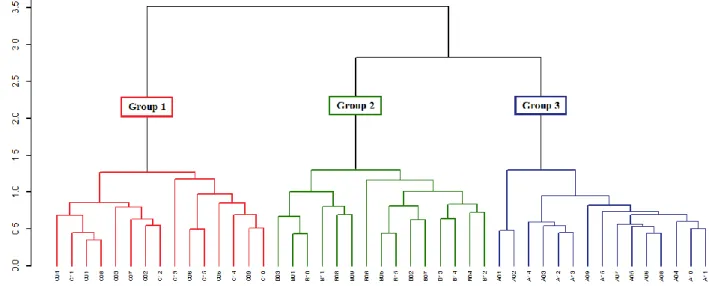
In general, the dendrograms generated by the different methods formed three well-defined groups, for the Euclidean, Squared Euclidean and Manhattan, distances. The groups formed are the same and consist of samples from the same archaeological site. For distance Mahalanobis, the groups formed are not well-defined and presented samples mixtures from different sites, which leads to false interpretations. To illustrate this fact, for example, two dendrograms were chosen, Manhattan distance with Average Linkage method and Mahalanobis distance with Complete Linkage method, respectively, in Fig. 1 and Fig. 2.
Figure 1: Dendrogram of the ceramics sample using Manhattan distance and Average
Linkage method.
Figure 2: Dendrogram of the ceramics sample using Mahalanobis distance and Complete
Linkage method.
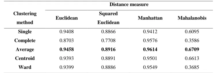
To validate and compare the clustering methods, the cophenetic correlation coefficient (CCC) was estimated, which measures the fit degree between the original dissimilarity matrix and the resulting matrix of simplification provided by the clustering method. Thus, the closer to 1 is the CCC, the better the grouping quality [6, 7]. According to Rohlf [21], in practice dendrograms with CCC less than 0.7 would indicate the inadequacy of the grouping method to summarize the data set information. These values are represented in Table 2.
Thus, the CCC value for the dendrogram of Fig. 3 is 0.3586, and it explains the false clustering. By comparing the CCC values, it can be observed that of the distance metric used does not matter and the Average Linkage method obtained better results, which corroborates with the literature [9, 22, 23].
Table 2: The cophenetic correlation coefficient values. Distance measure
Clustering
method Euclidean
Squared
Euclidean Manhattan Mahalanobis Single 0.9408 0.8866 0.9412 0.6095
Complete 0.8703 0.7708 0.9576 0.3586
Average 0.9458 0.8916 0.9614 0.6709 Centroid 0.9393 0.8891 0.9501 0.6613
Ward 0.9399 0.8886 0.9549 0.3685 Finally, to facilitate the statistical study of researchers who do not have much familiarity with statistical programs, the script developed becomes very useful, since it is enough to just insert the data set in the statistical program R and to execute it thus obtaining a table with all the cophenetic correlation values. This way, the researcher can easily check which method and distance is most appropriate for your data set. The Fig. 3 shows the screen generated by the script developed in this work.
4. CONCLUSION
Several clustering methods types are found in the literature, with the researcher deciding which is most suitable for their purpose, since the various methods combinations based on different dissimilarity measures can lead to different data set cluster. Based on the results obtained, it can be verified that for the Euclidean, Squared Euclidean and Manhattan distance associated to the five clustering methods studied in this work, the groups formed are the same, composed of samples from the same archaeological site and that the clustering quality for these distances is better than the clustering generated by the use of the Mahalanobis distance. At this distance the formed groups end up mixing samples from different sites, which leads to false interpretations. Moreover the results show that the method Average linkage was the one which has the best cophenetic correlation coefficient result. That was determined using a script developed that may be helpful to researchers find the most appropriate grouping method for their data set.
5. ACKNOWLEDGMENT
The author thanks the CAPES/PROEX for the financial support.
REFERENCES
1. FÁVERO, L. P.; BELFIORE, P.; SILVA, F. L.; CHAN, B. L. Análise de dados: modelagem
multivariada para tomada de decisões, Rio de Janeiro: Elsevier, 2009.
2. MINGOTI, S. A. Análise de dados através de métodos de estatística multivariada: uma
abordagem aplicada, Belo Horizonte: Editora UFMG, 2005.
3. PAPAGEORGIOU, J.; BAXTER, M. J. Model-based cluster analysis of artefact compositional data. Archaeometry, v. 43(4), p. 571-588, 2001.
4. TREBUNA, P.; HALCINOVÁ, J. Mathematical tools of cluster analysis. Applied
Mathematics, v. 4, p. 814-816, 2013.
5. HAIR Jr., J. F.; ANDERSON, R. E.; TATHAM, R. L.; BLACK, C. Análise multivariada de
dados, Porto Alegre: Bookman, 2005.
6. BARROSO, L. P.; ARTES, R. Análise multivariada, In: 48ª Região Brasileira da Sociedade
Internacional de Biometria – RBRAS, 9º Simpósio de Estatística Aplicada à Experimentação Agronômica – SEAGRO, Lavras, MG, 7 a 11 de julho, 2003.
7. BUSSAB, W. O.; MIAZAKI, E. S.; ANDRADE, D. F. Introdução à análise de
agrupamentos. São Paulo: ABE, 1990.
8. EVERITT, B. S.; LANDAU, S.; LEESE, M.; STAHL, D. Cluster analysis, London: Edward, 2011.
9. SARAÇLI, S.; DOGAN, N.; DOGAN, I. Comparison of hierarchical cluster analysis methods by cophenetic correlation. J. Inequalities and Applications, v. 203, p. 1-8, 2013.
10. MUNITA, C. S.; PAIVA, R. P.; ALVES, M. A.; OLIVEIRA, P. M. S.; MOMOSE, E. F. Provenance study of archaeological ceramic. J. Trace and Microprobe Techniques, v. 21(4), p. 697-706, 2003.
11. MURTAGH, F.; CONTRERAS, P. Methods of Hierarchical Clustering. Data Mining and
Knowledge Discovery, Wiley-Interscience, v. 2(1), p. 86-97, 2012.
12. FLOREK, K.; LUKASZEWIEZ, L.; PERKAL L. et al. Sur la liaison et la division des points d’un ensemble fini. Colloquium Mathematicum, v. 2, p. 282-285, 1951.
13. SNEATH, P. H. A. The application of computers to taxonomy. J. General Microbiology, v. 17, p. 201-226, 1957.
14. JOHNSON, S. C. Hierarchical clustering schemes. Psychometrika, v. 32, p. 241–254, 1967. 15. MARDIA, K. V.; KENT, J. T.; BIBBY, J. M. Multivariate Analysis, London: Academic Press,
1989.
16. WARD, J. H. Hierarchical grouping to optimize an objective function. J. Applied Statistics, v. 58, p. 236-244, 1963.
17. SOKAL, R. R.; ROHLF, F. J. The comparison of dendrograms by objective methods. Taxon, v. 11, p. 33-40, 1962.
18. VENABLES, W. N.; SMITH, D. M.; THE R CORE TEAM. An introduction to R, 2017. Available at: <https://cran.r-project.org/doc/manuals/r-release/R-intro.pdf> Last accessed: 10 Nov. 2017.
19. OLIVEIRA, P. M. S.; MUNITA, C. S. Influência do Valor Crítico na Detecção de Valores Discrepantes em Arqueometria, In: 48ª Reunião Anual Região Brasileira da Sociedade
Internacional de Biometria, Lavras, MG, Brazil, 07-11 de julho, 2003.
20. OLIVEIRA, P. M. S.; MUNITA, C. S.; HAZENFRATZ, R. Comparative study between three methods of outlying detection on experimental results. J. Radioanalytical and Nuclear
Chemistry, v. 283, p. 433-437, 2010.
21. ROHLF, F. J. Adaptative hierarquical clustering schemes”, Systematic Zoology, v. 19(1), p. 58-82, 1970.
22. KUIPER, F. K.; FISHER, L. A. A Monte Carlo comparison of six clustering procedures.
Biometrics, v. 31, p.777-783, 1975.
23. MILLIGAN, G. W.; COOPER, M. C. A study of standardization of variables in cluster analysis.