Assessment of edaphic community and distribution in cover vegetation of the Botanical Garden of Porto

Assessment of

edaphic community

and distribution in

cover vegetation of

the Botanical

Garden of Porto

Miguel Ângelo Oliveira Santos

Mestrado em Ecologia e Ambiente

2017

Orientador

Doutora Sara Cristina Ferreira Marques Antunes, Professora Auxiliar Convidada do Departamento de Biologia da Faculdade de Ciências da Universidade do Porto

Coorientador

Doutor Rubim Manuel Almeida da Silva, Professor Auxiliar do Departamento de Biologia da Faculdade de Ciências da Universidade do Porto

Todas as correções determinadas pelo júri, e só essas, foram efetuadas. O Presidente do Júri,

Dissertação submetida à Faculdade de Ciências da Universidade do Porto, para a obtenção do grau de Mestre em Ecologia e Ambiente, da responsabilidade do Departamento de Biologia.

A presente tese foi desenvolvida sob a orientação científica da Doutora Sara Cristina Ferreira Marques Antunes, Professora Auxiliar Convidada do Departamento de Biologia da FCUP; e co-orientação científica do Doutor Rubim Manuel Almeida da Silva, Professor Auxiliar do Departamento de Biologia da Faculdade de Ciências da Universidade do Porto.

Agradecimentos

Aos orientadores desta tese, Professora Sara Antunes e Professor Rubim Almeida, por todo o apoio e disponibilidade oferecida ao longo deste trabalho, sempre prontos a ajudar e a nunca me deixarem ficar baralhado ou desmotivado e, sem eles, esta tese não era possível, ficando aqui o meu profundo agradecimento.

Ao Professor Doutor Paulo Marques e a todos os funcionários do Jardim Botânico do Porto por autorizarem e permitirem a realização deste estudo, mostrando compreensão e disponibilidade na realização das amostragens.

À minha família, por me ter apoiado neste trabalho e de nunca ter duvidado de mim durante esta jornada de cinco anos que chega ao fim com a elaboração desta tese. Aos meus amigos mais próximos, Ricardo Alves, Pedro Fernandes, João Ferreira, Nuno Martins e Inês Bryant-Jorge, que são aqueles que tenho em consideração há mais tempo, cujos anos que nos conhecemos já não se contam com as mãos e que me alegraram e me apoiaram desde sempre.

Aos amigos da faculdade, Carlos Daniel, António Abade, Luís Silva, Luís Cunha, João Almeida, Gonçalo Leite, Pedro Rosa, Pedro Santos, Diogo Vale, João Osório e Raul Valente que me acompanharam ao longo destes cinco anos e que se tornaram praticamente família,

E, finalmente, aos meus colegas e amigos do Laboratório 1.14, Fábio Martins, Conceição Marinho, Guilherme Braga, Sérgio Ribeiro e Sara Rodrigues, que transformaram o ambiente de laboratório num de camaradagem, de forma a conseguir ultrapassar esta etapa da minha vida com maior gosto e facilidade.

Resumo

Os invertebrados terrestres desempenham um papel fundamental no funcionamento do solo, sendo responsáveis por vários processos ecológicos, nomeadamente acelerando a decomposição, mediando os processos de transporte e aumentando a atividade microbiana e fúngica. No entanto, a composição das comunidades edáficas pode ser influenciada pelo coberto vegetal existente. Assim, o objetivo deste estudo foi avaliar a composição e diversidade de invertebrados do solo em diferentes cobertos vegetais do Jardim Botânico da Universidade do Porto. Para tal, foram definidas dez zonas de amostragem dentro do Jardim Botânico com cobertos vegetais distintos (ex: áreas ajardinadas, áreas com vegetação arbórea diversa, área de suculentas). Para a avaliação da comunidade edáfica, foram colocadas armadilhas de queda (pitfall) em dois períodos distintos (outono e primavera). Adicionalmente, foi efetuada uma caraterização do solo através da quantificação de alguns parâmetros físicos e químicos: pH, condutividade, matéria orgânica, capacidade de retenção de água e textura. Na generalidade, os solos apresentaram uma natureza acídica (5,84 ± 0,63), e as áreas com maior cobertura vegetal apresentaram valores de condutividade, capacidade de retenção de água e de teor de matéria orgânica mais elevados. A comunidade edáfica apresentou valores de diversidade baixos, sendo menores que 1,5 e valores de equitatividade relativamente altos, superiores a 0,5. As zonas que possuem um maior coberto vegetal apresentaram uma maior diversidade da comunidade edáfica (Z1, Z6 e Z9). Os organismos observados com maior abundância pertenciam aos grupos Acari, Collembola e Hymenoptera (Família: Formicidae). Na análise de correspondência canónica efetuada para cada período de amostragem para as matrizes comunidade edáfica vs coberto vegetal não foi possível observar uma tendência similar na distribuição dos locais para os dois períodos de amostragem. O papel ecológico dos artrópodes poderia ser ainda mais explorado e compreendido através da realização de estudos ambientais semelhantes em diferentes habitats e tipos de perturbação, com foco em diferentes coberturas de vegetação.

Palavras-chave: Fauna edáfica, caracterização do solo, coberto vegetal, armadilhas pitfall, jardim botânico, índice de diversidade

Abstract

The terrestrial invertebrates play a fundamental role in soil functioning, being responsible for several ecological processes, namely accelerating decomposition, mediating the transport processes and increasing the microbial and fungal activity. However, the composition of edaphic communities can be influenced by the existing vegetation cover. Thus, the objective of this study was to evaluate the composition and diversity of soil invertebrates in different vegetation covers of the Botanical Garden of the University of Porto. For this purpose, 10 sampling zones were defined within the Botanical Garden with different vegetation cover (i.e.: garden areas, areas with diverse arboreal vegetation, succulent plants area). For the evaluation of the edaphic community, pitfall traps were placed in two distinct periods (autumn and spring). In addition, a soil characterization was carried out by quantifying some parameters: pH, conductivity, organic matter, water retention capacity and texture. In general, the soils presented an acidic nature (5.84 ± 0.63), and the areas with higher vegetation coverage had higher values of conductivity, water retention capacity and organic matter content. The edaphic community demonstrated low diversity values, all smaller than 1.5 and relatively high values of evenness, with values higher than 0.5. However, the zones that presented greater vegetal cover were those that displayed greater diversity of the edaphic community (Z1, Z6 and Z9). The organisms most abundantly observed belonged to the groups Acari, Collembola and Hymenoptera (Family: Formicidae). In the canonical correspondence analysis performed for each sampling period for the edaphic community vs. vegetation matrices, it was not possible to observe a similar trend in the distribution of the sites for the two sampling periods. The ecological role of arthropods could be further explored and understood through the conduct of similar environmental studies in different habitats and disturbances, with the focus on different vegetation coverages.

Keywords: Edaphic fauna, soil characterization, vegetation cover, pitfall traps, botanical garden, diversity index

Table of Contents

Introduction………1

Botanical Gardens………..………1

Arthropods & Ecology………..………..3

Soil, Edaphic Fauna & Ecology………..………..6

Vegetation, Edaphic Fauna & Ecology…………..………..7

Objectives………..………...9

Material and Methods………11

Study Area………..11

Sampling Procedures………12

Collection of Edaphic Community………..12

Vegetation Cover………..13

Laboratory Procedures……….14

Soil Characterization………14

Edaphic Community Characterization………..……….16

Data Analysis………..………..16 Results………18 Soil Characterization………18 Vegetation Analysis……….20 Edaphic Community ……….………..25 Discussion………..34 References……….40 Annex…..………51

Figure Index

Fig.1 – Sampling zones (Z1 to Z12) map of Porto’s Botanical Garden. Also represented is Casa Andresen (CA), the main building of the Botanical Garden. Adapted from Marques et al., 2015………..13 Fig. 2 – United States Department of Agriculture’s Soil Texture Triangle for the determination of soil texture……….16 Fig. 3 - Variation of pH values (Mean + SD) at each sampling site, during the Autumn and Spring sampling campaigns………...………..18 Fig. 4 - Variation of conductivity values (Mean + SD) at each sampling site, during the Autumn and Spring sampling campaigns………..…19 Fig. 5 - Variation of water holding capacity values (Mean + SD) at each sampling site, during the Autumn and Spring sampling campaigns ………...19 Fig. 6 - Variation of Soil Organic Matter Content (Mean + SD) at each sampling site, during the Autumn and Spring sampling campaigns.………20 Fig. 7 - Variation of abundance numbers at each sampling site, during the Autumn and Spring sampling campaigns……….27 Fig. 8 - Variation richness values at each sampling site, during the Autumn and Spring sampling campaigns……….28 Fig. 9 - Variation of the Shannon Diversity Index (Mean + SD) at each sampling site, during the Autumn and Spring sampling campaigns………29 Fig. 10 - Variation of the Pielou Equitability Index (Mean + SD) at each sampling site, during the Autumn and Spring sampling campaigns………29 Fig. 11 – Graphical representation of the Autumn CCA using the edaphic community composition and the vegetation coverage, following the nomenclature in Table 1 for the vegetation species and Table 2 for the edaphic families ………31 Fig. 12 – Graphical representation of the Spring CCA using the edaphic community composition and the vegetation coverage, following the nomenclature in Table 1 for the vegetation species and Table 2 for the edaphic families………32

Table Index

Table 1 – List of families and species of vegetation according to sampling zone, abundance and coverage percentage and in red, the exotic species. C.N.D. means Could Not Determine. An abbreviation (Abb.) was also created for each species to be used in the Canonical Correspondence Analysis.………...………22 Table 2 - List of invertebrate families encountered during the sampling procedures and their abbreviation used in the analysis of the edaphic community……….25 Table I – Occurrences and abundance of each invertebrate family encountered during the Autumn (AZ) and Spring (SZ) sampling seasons, in all sampling zones………...…...……….51

Introduction

Botanical Gardens

Botanical gardens have been a fundamental part of society for the last centuries. The first botanical gardens were built in Europe in the 16th _{Century when plant species were} brought back from recently discovered lands (Smith & Harvey-Brown, 2017). These botanical gardens served as a repository of botanic wealth, a place to evaluate and research these plant species for their economic and aesthetic value (Ward et al., 2010). Culturally botanical gardens are places for community members to interact with plants. While the first European botanical gardens were being developed, private homes and gardens were opening for public visitation. According to Connell (2005), such gardens were not developed for visitors but over time these gardens “adopted and adapted their

facilities for this function—the consumption of pleasure by the public” (p. 185). Public

interest in gardens grew in the 19th _{century as the increasing urban middle class} emulated upper class recreation pursuits (Constantine, 1981). Major cities established public botanical gardens in the 1800s, which also added to the growing public interest in garden visitation. As visitation steadily increased, the reasons for it evolved from a simple aesthetic desire to a complex blend of social, intellectual, and personal factors. In part, gardens create an opportunity to retreat from everyday modern life into a pleasant environment. These ideals are seen in other research that point to gardens as being spiritually satisfying and creating a tranquil environment for leisure consumption (Connell, 2005).

Approximately 200 million of people visit botanical gardens each year (Chang et

al., 2008). With 2500 botanical garden-related organizations spread throughout the world

(Ward et al., 2010), botanical gardens play a major role as research sites, hubs of biodiversity, tourist destinations and education centers, as well as by providing exposure to species and ecosystems that visitors may never otherwise experience. As a public learning institution, botanical gardens have “an increasing important role to play in

society, and the leisure aspect will provide an important medium through which people can acquire information, develop ideas and construct new visions for themselves and their society” (Packer & Ballantyne, 2002, p. 183). Botanical garden managers often

develop and maintain gardens with the premise that visitors frequent botanical gardens for educational purposes (Ballantyne et al., 2008). A large portion of garden resources is often dedicated to educating visitors about issues ranging from gardening techniques and skills to environmental awareness and resource conservation. However, studies on visitor motivations have shown that botanical garden visitors are often motivated to

pursue a wide range of leisure activities outside of horticultural interests (Nordh et al., 2011; Ward et al., 2010).

Of the many ways of defining a botanical garden, The Botanic Gardens

Conservation Strategy (Smith & Harvey-Brown, 2017) defines it as possessing the

following characteristics:

• A reasonable degree of permanence;

• A mandatory scientific basis for the collections;

• Proper documentation of the collections, including wild origin; • Monitoring of plants in the collections;

• Adequate labelling of plants; • Open to the public;

• Communication of information to other gardens, institutions and the public; • Exchange of seed or other materials with other botanic gardens, arboreta or research institutions (within the guidelines of international conventions national laws and customs regulations);

• Undertaking scientific or technical research on plants in the collections;

• Maintenance of research programs in plant taxonomy with associations of herbaria;

• Long term commitment to, and responsibility for, the maintenance of plant collections;

• Promoting conservation through extension and environmental education activities.

As botanical gardens maintain a wide collection of plant species, ranging from native to exotic plants, questions about conservation and plant invasions begin to surface. Botanical gardens are increasingly recognized as key players in global plant conservation through their living collections of endangered species, long-term archiving of seeds, taxonomic training and public outreach (Marris, 2006; Havens et al. 2006; Oldfield, 2009). Much less widely acknowledged is the role that they might have in both the deliberate and accidental introduction of invasive alien species, namely plants, across the globe (Reichard & White, 2001; Dawson, 2008; Heywood, 2011). Many of the first records in herbaria of naturalized aliens are from sites close to arboreta, botanical gardens, nurseries, or experimental planting (Wester, 1992). Even though when anybody mentions the words “Botanical Garden”, the subject that comes to mind is “plants”, botanical gardens’ importance is not only defined and measured by its plant diversity, but can also be defined by the abundance and populations dynamics of other living beings, such as birds and arthropods.

Arthropods & Ecology

Arthropods (from the Greek “arthro” (joint) and “podos” (legs), “jointed legs”) constitute one of the most diverse groups of organisms of the planet, comprising hundreds of thousands to several million species (Brusca & Brusca, 1990). There is still a large discussion in the scientific community regarding arthropod diversity and evolution, with new species being described every year (Ødegaard, 2000). The animals belonging to this group are known colonizers of basically every habitat, even unsuitable ones (Chinery, 1986). The first fossil records of arthropods date from Early Cambrian and the first arthropods were aquatic organisms which later radiated into the huge variety of aquatic and terrestrial forms known today. The origin and taxonomy of this group still constitutes a controversial field of research, and in the past few years, breaktroughs in molecular biology have been providing new insights regarding the group’s complex evolutionary relationships. Furthermore, arthropods are an extremely important group in terrestrial ecosystems due to not only their huge abundance and diversity but also the great number of essential environmental processes on which these organisms participate (Yi et al., 2012). Taking these factors into account, it is therefore of great importance the study of soil arthropods and their role in terrestrial landscapes (Kremen

et al., 1993).

The phylum Arthropoda, by far the largest of Animal Kingdom, is currently subdivided in five sub-phyla (Zhang, 2011): Trilobitomorpha, Crustacea, Myriapoda, Chelicerata and Hexapoda.

Sub-phylum Trilobitomorpha (trilobites and their relatives) comprises about 20000 species which lived exclusively in marine environments, and are all extinct. Their wide geographic distribution and hard calcium carbonate exoskeleton allowed this clade to present an extensive fossil record for all planet (Lieberman & Karim, 2010).

Crustaceans (including crabs, shrimps and lobsters), containing more than 60 000 species, establish one of the major arthropod groups. Most crustaceans live in marine environments, but several species can be found in freshwater ecosystems and in terrestrial environments (order Isopoda). Despite most crustaceans being free-living, there are several groups of parasitic forms. This group also presents an extensive fossil record, first appearing in Middle Cambrian (Schram, 1982). On a different approach, some decapod crustaceans, such as lobsters and shrimps have significant economic importance, being consumed worldwide.

The sub-phylum Myriapoda, including the centipedes and millipedes, contains over 11 000 described species (Zhang, 2011). This sub-phylum is traditionally divided in four Classes: Chilopoda (centipedes), Diplopoda (millipedes), Pauropoda and Symphyla

(pseudocentipedes). All existing myriapods are terrestrial, but these organisms are not as well adapted to life on land as spiders or insects. Their size ranges from a few millimeters to around 38 centimeters (Giant African Millipede) (Brusca & Brusca, 1990). The sub-phylum Chelicerata (including spiders, sea spiders, scorpions, mites, harvestmen) contains over 113 000 species (Zhang, 2011) placed in two main Classes: Pycnogonida (sea spiders) and Arachnida (spiders, scorpions, mites, thicks). Pycnogonida, the group of the sea spiders, contains more than 1 300 described species, but detailed studies regarding these animals and their taxonomic relationships are still scarce (Arango & Wheeler, 2007). These organisms usually have six or eight eyes and four to six pair of legs attached to a small body. The class Arachnida comprises the most well-known organisms of the Chelicerata sub-phylum, such as spiders, scorpions or mites. The individuals included in this group have four pairs of legs, chelicerae and pedipalps, all the appendages being multiarticulate and antennae are absent (Brusca & Brusca, 1990). Spiders (Order Araneae) are probably the most iconic and well-studied group of Cheliceriformes, present in most terrestrial environments and constituting one of the most important groups of soil arthropods. Other organisms placed in the same Class, such as scorpions (Order Scorpiones), mites (Order Acarina) or harvestmen (Order Opiliones) also establish extremely diverse groups with important ecological functions (Cloudsley-Thompson, 1958).

The sub-phylum Hexapoda (“Hexa” (six) and “Poda” (foot)), insects and their relatives, comprises the most diverse and abundant groups of organisms with over 1 million recorded species (Zhang, 2011). This clade is commonly divided into insects (Class Insecta) and related wingless organisms: Springtails (Collembola), coneheads (Protura) and two-pronged bristletails (Diplura) belong to the class Entognatha and are thought to be the most primitive hexapods. These organisms are entognathous, meaning their mouthparts (unlike the insects, which are ectognathous) are retracted within their heads (Grimaldi & Engel, 2005). Proturans are small soil dwelling organisms usually under 2 mm long with no eyes, antennae or ocelli. Springtails constitute one of the most abundant groups of soil arthropods, in a square meter of more than 100 000 collembolans can be found. These are cosmopolitan organisms, over 8 000 species described, making springtails the most diverse apterygote group. Collembolans are small organisms, their size usually under 6-8 mm, cylindrical or globular-shaped, presenting simple eyes composed of up to eight ocelli and moniliform antennae. Many species possess a forked tail-like appendage (furcula) in the end of the abdomen, which allows springtails to jump in the air when threatened. Collembolans have been widely used in ecotoxicological assessments regarding soil quality and overall health of these ecosystems (Hopkin, 1997).

Insecta is the biggest Class of animals, comprising more than half of the described eukaryotic species. This Class encompasses over 1 million species which are virtually thought to inhabit every terrestrial ecosystem and some freshwater and marine environments. Insects are by far the most diverse group of living creatures, showing an enormous diversity of organisms and adaptations (Chinery, 1986). Alongside the extreme diversity in this clade, insects are also extremely abundant. It is estimated a number of 200 million insects per human being on the planet. Their tremendous richness and abundance is thought to be the result of a combination of advantageous features, such as the coevolution with plants, miniaturization and flying ability (insects are the only invertebrates able to fly, which allows them to occupy more ecological niches). Being such an abundant group, insects play a major role in ecosystem functioning. They are predators of many other invertebrate groups and food source for numerous vertebrates, being of great importance in terrestrial food webs. Numerous flying insects, such as bees or butterflies, act as pollinators of many plant species. This is a very important ecological function with several economic repercussions because more than 30% of the world’s food crops depend on animal pollinators. Some groups of insects also play an important role in the maintenance of soil structure and functioning (Brusca & Brusca, 1990).

Insects also play a very important part in scientific research. Typical features such as their small size, short generation time and high fecundity make insects suitable candidates for research purposes. For example, the fruit fly, Drosophila melanogaster, is one of the most studied organisms in cellular and molecular biology (Jennings, 2011; Markow, 2015). Its genome is known to science and researchers use this species to investigate several cellular processes (Adams et al., 2000). Despite making up such an interesting group, there are some disadvantages associated with insects. Mosquitoes, sandflies and many other insects act as vectors of a significant number of diseases, causing the death of millions of humans and other vertebrates every year. For instance, malaria, the most widespread parasitic disease, with several million infected humans around the globe, is transmitted by the bite of Anopheles mosquitoes (Cameron & Lorenz, 2013). In agriculture, insect pests are responsible for damaging of agricultural crops and food production causing significant economic losses every year (Caballero et

al., 2015). There is a significant number of insect alien invasive species that can affect

native biodiversity and ecosystem functioning through a variety of mechanisms. However, this is a research field where more work needs to be conducted since the vast majority of published studies regarding the impact of insects as invasive organisms have only focused on a small number of species (Kenis et al., 2008).

Soil, Edaphic Fauna & Ecology

The soil is an extremely dynamic, complex, and highly heterogeneous system that allows the development of an extremely large number of ecological habitats. Soil is the home of a vast spectrum of organisms, that perform important functions for the ecosystem (Gardi & Jeffery 2009).

Soil can be defined as a natural body made of a solid (minerals and organic matter), liquid and gaseous portions that occur on the surface of the planet (Brady & Weil, 1996). These natural systems can also be a set of mineral and organic material on the land surface that allows the growth of terrestrial plants. The latter is subjected to potential genetic and environmental factors, such as climatic influence and the action of organisms that inhabit soils and constitute the edaphic fauna (Soil Science Glossary Terms Committee, 2008). Soil ecosystem constitutes some of the most heterogeneous habitats in our planet showing a tremendous diversity, and they are crucial for the maintenance of a great number of ecosystem services. They play a fundamental role in insuring the existence of food and other materials, nutrient cycling, primary production, flood control and present many cultural and aesthetic values. Therefore, it is essential to promote the optimal ecological state of these entities which support the life of a large array of species (Millennium Ecosystem Assessment, 2005). This can be a difficult task due to the physical complexity and difficult accessibility of some soil systems, the lack of knowledge regarding soil organisms and their role in ecosystem functioning (Wall et al., 2012).

Soil biota (the organisms that usually live in soils) are typically sub-divided according to the size of the organisms into micro, meso, macro and megafauna (Wallwork, 1970). Soil microfauna comprises the organisms whose body size usually ranges from 2 to 200 μm and includes bacteria, fungi, nematodes and protozoans. Mesofauna comprises animals with a size variation between 200 μm and 2 mm. Invertebrates such as springtails and mites are the most abundant organisms in this group that also includes rotifers, tardigrades, small spiders, pseudoscorpions, opiliones, enchytraeids, small woodlice and myriapods. Macrofauna includes animals like the majority of insects, earthworms, isopods, myriapods and spiders, whose size ranges from 2 to 20 mm. Megafauna comprises animals whose body size is over 2 cm including large invertebrates and vertebrates such as small mammalians, amphibians or reptiles.

In terms of abundance and diversity, microorganisms (bacteria and fungi) and invertebrates (nematodes, arthropods, enchytraeids and earthworms) are known to be among the most relevant groups in soil ecosystems (Jeffery et al. 2010). In the soil, these organisms have key functions in organic matter decomposition, the nutrient cycle, the

enhancement of soil structure, and the control of soil organisms, including crop pests (Moore & Walter 1988) and important components of soil food webs (Gardi & Jeffery 2009; Jeffery et al. 2010). However, soil organisms also contribute to the regulation of atmospheric composition and climate, water quantity and quality, and the reduction of environmental pollution (Gardi & Jeffery 2009; Jeffery et al. 2010; Lavelle et al. 2006). According to these functions, soil edaphic communities have been divided in three wide functional groups, i.e., chemical engineers, biological regulators, and ecosystem engineers (Turbé et al. 2010; Lavelle et al. 2006). These organisms are capable of altering soil physical and chemical structure and other properties of the surrounding environment. Soil invertebrates are known to participate in water supply, nutrient cycling and soil formation, flood and erosion control and climate regulation (Lavelle et al., 2006). On the other hand, soil arthropods respond very quickly to changes in the environment, and results obtained from arthropod studies can be used to characterize accurately almost any aspect of an ecosystem (Kremen et al. 1993).

The interactions established between edaphic organisms and their surrounding environment varies between taxa and the part of life cycle that each organism spend time in the soil. When considering the ecology of the different organisms and morphological adaptations of soil fauna is usually classified in four groups. Temporary inactive geophiles, are animals that only live in the soil for some phase of their life cycle, for example to undergo metamorphosis or when looking from protection for unfavorable climatic conditions. On the other hand, temporary active geophiles live in the soil for most of their life cycle (several life stages). Periodical geophiles live in the soil during one part of their life cycle, usually as larvae, and they occasionally return to the soil, to fulfill several activities, such as hunting or laying eggs. Geobionts are organisms well adapted to live in soils and they cannot leave this environment, even temporarily, because these animals do not have adaptations that allow their survival above the surface. According to this classification, it is expectable that changes in the quality of soil ecosystems will not impact all the groups in the same way. A geobiont, which spends the entirety of its life cycle below the surface, is in theory more susceptible to soil contamination or other impacts than temporary inactive geophiles, which only spend a part of their life cycle living underground (Wallwork, 1970).

Vegetation, Edaphic Fauna & Ecology

Vegetation can also be a major influence in the life cycle of the organisms that comprise the edaphic fauna, affecting their distribution and population dynamics (Kaufmann, 2001). Plants act as an extension of the soil and, in return, define it, since their coverage

changes the properties of the soil itself (Zheng, 2006; Feng, 2016). As mentioned above, plants are also capable of affecting the lives of invertebrates, especially the ones living in the soil, for example, changing their shelter and predatory habits (Rodrigues et al., 2017; Sterzyńska et al., 2017).

In many studies conducted throughout the years, abundance and arthropod diversity variations were attributed to different vegetation structures (May, 1978; Morse

et al., 1985; Williamson & Lawton, 1991). Among arthropods, spiders are prime

candidates for showing the influence of vegetation in an arthropod life cycle. Especially in edaphic communities since the vegetation can be used as a hiding and breeding place, and as a means of hunting and moving (Greenstone, 1984; Gunnarsson, 1992). Interactions between the vegetation structure and other processes such as predation and competition may be of major importance in edaphic communities.

Small-scale vegetation structural complexity plays a key part in shaping grassland invertebrate assemblages (Morris, 2000). Habitat complexity is associated with features such as availability of foraging sites, shelter and overwintering or nesting sites, indicating abundance of resources (prey, pollen or nectar) and suitable refuges from predators, intra-guild cannibalism and competitors (Halaj et al., 2000; Langellotto & Denno, 2004; Finke & Denno, 2006). Habitat complexity (soil-vegetation-arthropods) might also be considered an explanatory factor in species–area relationships (Hart & Horwitz, 1991). Enhanced structural complexity may offer greater space–size heterogeneity, providing habitable space to organisms with a wide range of body sizes, thereby increasing species richness (Tokeshi & Arakaki, 2012; Pierre & Kovalenko, 2014).

Some invertebrate groups, namely generalist predators and spiders, appear to prefer more complex habitats (McNett & Rypstra, 2000; Shrewsbury & Raupp, 2006), with spiders negatively affected when habitat structure is simplified (Marshall & Rypstra, 1999; Langellotto & Denno, 2004; Wise, 2006). Ground-dwelling spider communities respond to commonly measured structural attributes such as height, above-ground biomass, vegetation tip height diversity and depth of plant litter layer (Uetz et al., 1999; Traut, 2005; Pétillon et al., 2008), but do not exhibit strong host-plant associations. Both phytophagous and predatory beetle habitat preferences are associated with commonly measured attributes of vegetation structure (Lassau et al., 2005; Hofmann & Mason, 2006; Woodcock et al., 2007) and satellite-derived vegetation indices (Lafage et al., 2014). Plant species richness may also contribute to vegetation structural complexity, and affect the abundance and species richness of predatory arthropods such as spiders and predatory beetles via bottom-up trophic effects (Scherber et al., 2010). A

species-rich plant community tends to support a large number of herbivorous arthropods, which in turn boost the predatory arthropod population (Borer et al., 2012).

The ‘enemies hypothesis’ (Root, 1973), proposes a mechanism of top-down control in which diverse vegetation assemblages provide more refuges for predatory arthropods and more opportunity for stable prey availability than low plant diversity assemblages (Russell, 1989). The habitat heterogeneity hypothesis (Dennis et al., 1998) predicts an asymptotic relationship between increasing plant species richness and vegetation structural heterogeneity, with greater resources available for the coexistence of multiple species of arthropods of each trophic group in structurally complex vegetation. Ground and canopy-dwelling invertebrates are sensitive to seasonal changes in environmental characteristics, such as changes in vegetation structure due to natural dieback in winter, but seasonal invertebrate–vegetation structure relations are rarely quantified. Dense vegetation may be more important for different reasons in winter than in the summer. For example, tussocky grasses (bundles of singular plants) and leaf litter provide overwintering shelter from predators for ground-dwelling invertebrates, including wolf spiders (Edgar & Loenen, 1974; Collins et al., 2002; Lewis & Denno, 2009), whereas in spring and summer, prey availability is often crucial (Wise, 2006), encouraging individuals to explore more open habitat. Tall vegetation offers several benefits for invertebrates, including protection from predation and shelter from extreme weather events. However, daytime temperatures are lower in tall vegetation, potentially hindering thermophilic invertebrates, inhibiting movement and hiding prey, especially in dense grass mats such as Festuca rubra L. swards (Van Klink et al., 2015). Hence, vegetation that is tall, but not dense may be optimal.

Objectives

The Botanical Garden includes different compartments (soil, fauna and flora) that have an important function on the health of this urban ecosystems. According to this, the scope of this study was to characterize the edaphic community in different vegetation coverage of the Botanical Garden of Porto University. Keeping in mind this goal, the present study defined the following objectives:

• identify and distinguish the different vegetation covers in the Botanical Garden of Porto (BGP);

•

•

•

Material and Methods

Study Area

The first Botanical Garden in Porto was established by decree of Passos Manuel in 1837, being located in the extinct Carmelite Convent (1852), although its creation was only verified in 1866. With the expansion of the Municipal Guard’s barracks, the Garden was installed in 1903 in Cordoaria, for a short period being the University of Porto deprived of its garden for half a century. The BGP was installed in the actual place “Quinta do Campo Alegre”, since 1951 with a total area of 12 ha (Jardim Botânico do Porto (JBP), 2017).

This farm belonged initially to the Order of Christ and was acquired in 1802 by John Salabert to be known as the Great Fifth of Salabert. In 1820, it became the property of João José da Costa. In turn, João da Silva Monteiro acquired it in 1875 and began the construction of the central house and the garden. The farm was bought in 1895 by João Henrique Andresen Júnior, who continued to build the house and the garden. The farm remained in the possession of his family until 1949, when the sale to the Portuguese State was done. Professor Américo Pires de Lima, with the collaboration of the german Franz Koepp, after the purchase of Quinta do Campo Alegre by the State, adapted it, to the liking of the recreational farms of the city of Porto. The property was crossed by Arrábida’s Bridge accesses in 1956 and it was reduced to 4 ha. However, the property having conserved the initial gardens, and in the remaining part of the fields. On the other hand, the forest was being installed, along with new gardens, namely of succulent plants as well as an arboretum (JBP, 2017)

In 1983, the Botanical Garden closed to the public in the aftermath of its degradation, having reopened in 2001, after a first intervention to contain this degradation. The opportunity for an application to the ON Program (CCDRN) allowed renewing the networks of roads, watering, drainage and electricity, and several other improvements were also possible. The work forced the closure of the garden to the public in July 2006 making it possible to conclude this new phase of the intervention in May 2007 and thus reopening it. The BGP today has importance for its botanical aspect, possessing a significant set of species both for its rarity and its size, namely exotic species. It is still representative of the recreational farms of the nineteenth century’s Porto and is also a literary space. It is a place of reference in the life and work of the writers Sophia de Mello Breyner Andresen and Ruben A. (JBP, 2017).

Most recently, having its base in House Andresen, the Hall of Biodiversity opened to the public on June 30, 2017, by His Excellency the President of the Portuguese Republic Marcelo Rebelo de Sousa, becoming the first Ciência Viva Center specifically

devoted to biodiversity. In it visitors can encounter a wide range of sensorial experiences that combine art, history and biology, with the purpose of celebrating diversity of life. It also became the first museum created according to the total museum philosophy, cementing the role of the Garden in education and scientific research (Museu de História Natural e da Ciência da Universidade do Porto (MHNC-UP), 2017)

Currently, with 4 ha, the Botanical Garden is organized in three levels with very different characteristics. On the first level, involving the Andresen House, the formal gardens are developed, separated by the high hedges of centenary camellias, and influenced by the Arts and Crafts movement. On the second level, there is the garden of xerophytic plants with various cactuses and succulent plants, where we can find the canteens greenhouse, the tropical greenhouse and the orchid greenhouse. Finally, at the lower level, the arboretum is located, in which are the collections of conifers, autochthonous plants, the fetal and the largest lake of the Garden. All the different varieties of plants form two distinct patterns of vegetation cover in the Botanical Garden, such as the man-made gardens, typically with small plant coverage, mainly shrubs and herbaceous specimens and the bigger plant coverage, mainly found in the back of the garden, where most of conifers and autochthonous plants reside (JBP, 2017).

Sampling Procedures

Collection of Edaphic Community

In the BGP, 12 sampling zones were defined (Figure 1 - Z1 to Z12), with different vegetation cover and characteristics (between landscape to “natural” areas) (Figure 1). The sampling process was done in two distinct occasions, one during Autumn (October 2016) and another in Spring (April 2017). The sampling periods were established by considering the time of year in which the edaphic community is more active (André et al., 2009).

Fig.1 – Sampling zones (Z1 to Z12) map of Porto’s Botanical Garden. Also represented is Casa Andresen (CA), the main building of the Botanical Garden. Adapted from Marques et al., 2015.

To characterize the edaphic community present in the BGP, four pitfalls traps were randomly placed at each sampling site, totaling 48 pitfall traps. Pitfall traps used in this study were made from a cylindrical plastic container, usually comprised of the bottom portion of 1.5 L water bottles, with a diameter of 7.5 cm and height of 8 cm. A mixture of water and formaldehyde (4% v/v) was placed in the traps to kill and preserve the organisms. A few drops of detergent were added to break the surface tension, allowing the captured organisms to sink to the bottom of the traps. Pitfalls were placed in the soil and then covered with stones, small pieces of wood and leafs to minimize rainfall entrance, prevent the capture of small vertebrates and possible human disturbance. Pitfall traps remained on the field for 11 days (Pereira et al., 2008). After this time, pitfall content was filtered using a 200 μm net funnel and then stored in individual flasks containing a 70% alcohol solution to preserve the collected organisms until posterior taxonomic identification.

Vegetation Cover

In each sampling zone, ranging from landscaped areas to more “natural” ones, vegetation was identified, as well as counted and their coverage percentage over each sampling zone was considered. This process was done through the creation of a 1 m2

square around the pitfall traps. Vegetation species inside the squares were listed as mentioned above, with the purpose of determining the influence of each, in the distribution of the edaphic community.

Laboratory Procedures

Soil Characterization

To place the pitfalls on the ground, an amount of soil was collected from each sampling site (four soil samples per sampling zone) and placed in litter bags. Litter bags containing soil samples were taken to the laboratory and remained open during one week for air drying to lose humidity. After this preliminary treatment, the following soil parameters were determined in the soil samples: pH, electrical conductivity (µS/cm), organic matter content (%), water holding capacity (%), and texture.

Soil pH is an evaluation of the hydronium ion (H3O+ or H+) activity in a soil solution (Tan, 2010) and pH can be defined as the negative logarithm (base 10) of H+ activity in a solution (pH= 1/log10 [H+]). This parameter is more than a simple indication of the acidity or alkalinity of a solution as, for example, availability of essential nutrients and toxicity of other elements can be estimated according to their relationship with soil pH (Thomas, 1996). The measurement of the pH was conducted following the International Organization for Standardization (ISO) guidelines (1994). Each soil sample (10 g) was added to a cup containing 50 mL of distilled water. The samples were placed on an automatic shaker for continuous agitation for 30 minutes. After this period, one-hour resting for the solutions was followed. After this time, pH values were determined using a multi-parametric probe (pH 1000L).

Conductivity can be defined as the ability of a material to conduct an electrical current. Soil conductivity (μS/cm) is a measure of the level of soluble salts found in a soil solution and it is therefore an important parameter to establish the quality of a soil sample since the concentration of several ions in solution might have several implications in the soil system (Jones, 2001). The conductivity of soil samples was assessed in the soil samples (soil + dH2O) used in pH (dH2O) assessment. After the measurement of pH, samples were left overnight, and in the next day electrical conductivity was measured using a conductivity probe (Consort 3030) (ISO, 1985).

Soil organic matter comprises any material that is produced by living organisms and is returned to soil, suffering partial or total decomposition. Based on their organic matter content, soils can be characterized as mineral or organic (the last ones containing higher amounts of organic matter) (Bot & Benites, 2005). Organic matter content is an important indicator of soil health, affecting the chemical and physical properties of soil,

such as its structure and porosity, diversity of soil organisms that can be found and plant nutrient availability (Bot & Benites, 2005). Organic matter content was estimated by loss on ignition (Davies, 1974). In this procedure 25 g (Dry Weight) of air-dried soil were weighted into crucibles (Tare) and were set in a muffle furnace for overnight burning at 450ºC. Following muffle burning, soil samples were put in a kiln and their weight was assessed (Muffle Weight). Organic matter content (%) was calculated accordingly to the equation (United States Environmental Protection Agency (USEPA), 2004):

𝑂𝑟𝑔𝑎𝑛𝑖𝑐 𝑀𝑎𝑡𝑡𝑒𝑟 (%) =(Dry Weight − Tare) − (Muffle Weight − Tare)

(Dry Weight − Tare) × 100

Soil water holding capacity constitutes a very important feature regarding soil structure and it is influenced by several characteristics of soil systems, such as surrounding vegetation and organic matter content (Naeth et al., 1991). To determine soil water holding capacity, soil samples (air dried) were weighted and placed into a cup where the bottom was replaced by filter paper (Tare). This set was sunk in a tray filled with water for three hours. After this period, the soil/cup assembly was removed from the basin to drain the excess of water and the weight of the samples was assessed again (Wet Weight). Soil samples were then placed in an oven at 60°Cfor a couple days until constant weight and then they were weighted again (Dry Weight). Water Holding Capacity was calculated using the following equation (ISO, 2008):

Water Holding Capacity (%) =(Dry Weight − Tare) − (Wet Weight − Tare) (Dry Weight − Tare) × 100

The mineral components of soil are sand, silt and clay, and their relative proportions determine the soil's texture. Properties that are influenced by soil texture, include porosity, permeability, infiltration, shrink-swell rate, water-holding capacity, and susceptibility to erosion. Soil texture was determined using the United States Department of Agriculture’s (USDA) Soil Texture Triangle (Figure 2), resulting in a soil type based on the percentages of sand, silt and clay present in each soil sample. After removing the organic matter by incineration from the samples, each sample was sieved to separated three different fractions using different sized sieves, >1mm, >50 µm and <50 µm, representing the sand, silt and clay portions, respectively.

Fig. 2 – United States Department of Agriculture’s Soil Texture Triangle for the determination of soil texture (USDA, 2017).

Edaphic Community Characterization

The content of each pitfall was then screened in the laboratory using a stereomicroscope to separate edaphic organisms from other materials, such as leaves and small pieces of wood. Following this preliminary stage, all adult organisms were identified to the taxonomic level of Family whenever possible, using specific identification keys (Bland & Jaques, 1978; Barrientos, 1988; Chinery, 1993; Roberts, 1995), with Barrientos (1988), being the main source of information for the identification of the edaphic organisms. The organisms belonging to the Diptera orders and other non-edaphic organisms were excluded from this characterization.

Data Analysis

The structure and composition of edaphic community were analyzed through descriptive statistical methods in Microsoft Excel®. Using this software, Shannon-Wiener Diversity Index and Pielou Equitability Index were determined for each replicate at all sampling locations, allowing posterior comparisons between different sampling locations in both sampling seasons.

Shannon-Wiener Diversity Index is a measure of diversity of biological communities widely used in ecological studies. Diversity indexes are quite useful since

they provide more information than a simple sum of the number of species. This biodiversity metric considers the number of taxa (richness) and the relative proportion of each group (abundance) of the desired community (Tramer, 1969). Shannon´s Index can be calculated according to the equation:

H’ = -Σ (Pi log[Pi])

where H’ is Shannon´s Index and Pi is a percentage of individuals of species i in the total number of individuals.

The evenness of arthropod communities was also assessed. Evenness can be defined as the distribution of the individuals between the different taxa in a certain community. The evenness of a community can be defined as a measure of the homogeneity of abundances of the different taxa (Levin et al., 2009). Several indexes have been proposed to determine the equitability of a certain community from its diversity (Heip et al., 1998). Pielou Equitability Index is one of the most widely used methods for the calculation of evenness. It ranges from 0 to 1, as the index increases so does the evenness of the community. It can be calculated using Shannon´s Diversity Index, according to the following equation:

J’= H’/H’ max= H’/log S

Where J’ is Pielou Equitability Index; H’ is Shannon’s Diversity Index and S the total number of taxa recorded in the community.

To assess the relationship between the edaphic community and the vegetation coverage percentage in each sampling season, two Canonical Correspondence Analysis were performed using Canoco® software for Windows 4.5. CCA is a multivariate analysis technique that can be used to study possible relationships between assemblages of species and a set of environmental factors (Ter Braak & Versonschot, 1995).

Results

Soil Characterization

The BGP’s soil status was studied through the determination of several soil parameters in two sampling seasons (Autumn and Spring). In each study zone, four soil samples were collected and the physical and chemical parameters were determined in laboratory. In Figure 3 are presented the pH values determined. Overall the sampling zones presented acidic soils in both sampling seasons. Moreover, the pH values between the two sampling campaigns were similar. Regarding the Autumn sampling season, pH values ranged from 5.27 in Z11 to 6.59 in Z8. The highest values were recorded in to Z6 (6.25), Z3 (6.53) and Z8 (6.59), while the lowest ones were observed in Z11 (5.27). The Spring campaign present a pH values ranging from 5.03 in Z11 to 6.57 in Z8. Zones Z6 (6.35), Z3 (6.38) and Z8 (6.57) reprising their role as the ones with the highest pH values, and zone Z11 (5.03) representing the zone with the lowest pH level.

Fig. 3 - Variation of pH values (Mean + SD) at each sampling site, during the Autumn and Spring sampling campaigns.

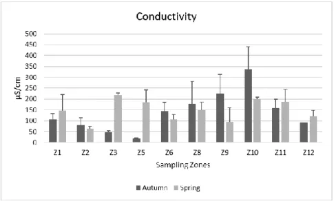
Conductivity values, can be observed in Figure 4. The data here-obtained were generally high, according to Möller et al. (2005) in both sampling season. However, a few exceptions were observed with lower conductivity values, namely in zones Z1, Z2, Z3, Z4, Z5 and Z12, particularly in the Autumn campaign. The conductivity values recorded in Botanic garden ranged from 20.05 µS/cm in Z5 to 338.57 µS/cm in Z10. When regarding the Spring season, conductivity values were generally lower, with zone Z2 presenting the lowest values (62.6 µS/cm) and zone Z3 with the highest value recorded (219.3 µS/cm). Zones Z1, Z3, Z5, Z11 and Z12, showed an increase in conductivity values from the Autumn to the Spring sampling period.

Fig. 4 - Variation of conductivity values (Mean + SD) at each sampling site, during the Autumn and Spring sampling campaigns.

The data in Figure 5 shown the water holding capacity (WHC) values. Overall the Autumn values are higher than the Spring season ones. The lowest value recorded was 8.33% in Z12 and the highest 27.98% in Z10, in the Autumn sampling. In the Spring sampling period, the lowest value observed was 6.28% in Z10 and the highest was 15.43% in the Z6 zone.

Fig. 5 - Variation of water holding capacity values (Mean + SD) at each sampling site, during the Autumn and Spring sampling campaigns.

Through the observation of Figure 6, and according to USEPA guidelines (2004), the soils collected in the Botanical Garden have a high content of organic matter (OM) (above 6%), except for Z5. Zone Z5 presented the lowest organic matter content in both sampling seasons. Regarding the Autumn campaign, the values of organic matter varied

between 5.34% in Z5 and 39.13% in Z10. Overall the soil samples collected in the Spring season having the highest values of organic matter. The highest value recorded were in Z10 (23.05%) and Z11 (18.25%), both like the autumn sampling, and Z5 was again the zone with the lowest value of OM.

According to the Soil Texture Triangle diagram classification (Figure 2), the texture of the different soil samples was determined. The textures of all the soil samples were classified as silt loam, since they all contain approximately 70% or more of silt and clay, and less than 30% of sand. This situation was verified in both sampling periods.

Fig. 6 - Variation of Soil Organic Matter Content (Mean + SD) at each sampling site, during the Autumn and Spring sampling campaigns.

Vegetation Analysis

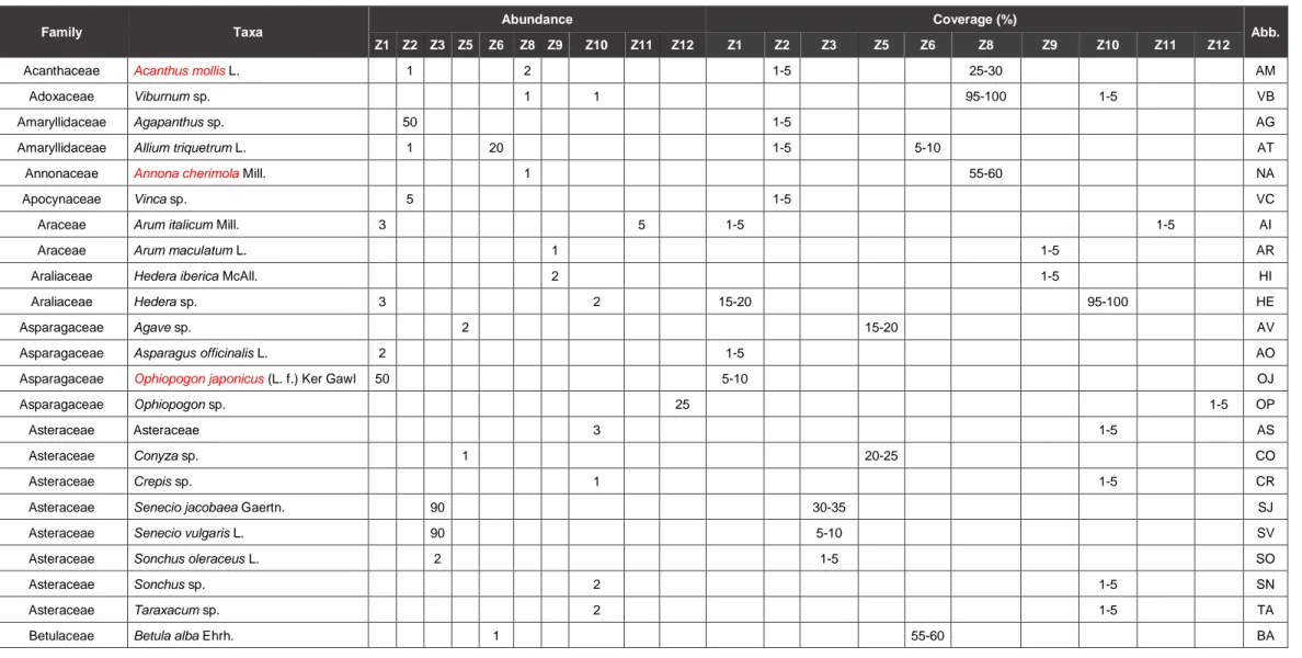
A floristic list was performed for each sampling zone with the quantifications of the following parameters: number of species, number of individuals and coverage percentage for each species (Table 1). The vegetation species richness was also considered and listed below alongside an abbreviation code for each species (Table 1). In the 10 sampling zones of the Botanical garden 69 species of plants were identified. An interpretation of their origin was also made, to separate autochthonous from exotic species (Table 1 - red color). The zone Z8 present the highest richness value with 21 different species observed, while Z12 shows the lowest number of species (n=3). The family most represented in the studied zones of the Botanical garden is the Asteraceae. In terms of coverage percentage, several species achieved 100%, or close to that value, namely Corylus avellana, Cupressus nootkatensis, Podocarpus sp. and

Camellia japonica in zones Z1, Z8, Z9 and Z11. The most observed species in the

sp. (Z10) could not be accounted for, presenting only its coverage percentage (Table 1). Zones Z6, Z9, Z10, Z11 and Z12 can be characterized by arboreous areas with the majority of the vegetation with a treelike structure, achieving higher coverage percentages. Zones Z1, Z2 and Z8 can be described as a mix of herbaceous and arboreous species. Zone Z3 is a fully herbaceous and shrub area, consisting of formal gardens. The more different zone is zone Z5 with a botanical collection with succulent plants.

Table 1 - List of families and species of vegetation according to sampling zone, abundance and coverage percentage and in red, the exotic species. C.N.D. means Could Not Determine. An abbreviation (Abb.) was also created for each species to be used in the Canonical Correspondence Analysis.

Family Taxa

Abundance Coverage (%)

Abb.

Z1 Z2 Z3 Z5 Z6 Z8 Z9 Z10 Z11 Z12 Z1 Z2 Z3 Z5 Z6 Z8 Z9 Z10 Z11 Z12

Acanthaceae Acanthus mollis L. 1 2 1-5 25-30 AM

Adoxaceae Viburnum sp. 1 1 95-100 1-5 VB

Amaryllidaceae Agapanthus sp. 50 1-5 AG

Amaryllidaceae Allium triquetrum L. 1 20 1-5 5-10 AT

Annonaceae Annona cherimola Mill. 1 55-60 NA

Apocynaceae Vinca sp. 5 1-5 VC

Araceae Arum italicum Mill. 3 5 1-5 1-5 AI

Araceae Arum maculatum L. 1 1-5 AR

Araliaceae Hedera iberica McAll. 2 1-5 HI

Araliaceae Hedera sp. 3 2 15-20 95-100 HE

Asparagaceae Agave sp. 2 15-20 AV

Asparagaceae Asparagus officinalis L. 2 1-5 AO

Asparagaceae Ophiopogon japonicus (L. f.) Ker Gawl 50 5-10 OJ

Asparagaceae Ophiopogon sp. 25 1-5 OP

Asteraceae Asteraceae 3 1-5 AS

Asteraceae Conyza sp. 1 20-25 CO

Asteraceae Crepis sp. 1 1-5 CR

Asteraceae Senecio jacobaea Gaertn. 90 30-35 SJ

Asteraceae Senecio vulgaris L. 90 5-10 SV

Asteraceae Sonchus oleraceus L. 2 1-5 SO

Asteraceae Sonchus sp. 2 1-5 SN

Asteraceae Taraxacum sp. 2 1-5 TA

Betulaceae Corylus avellana L. 1 95-100 CA

Cannaceae Canna indica L. 5 1-5 CI

Caryophyllaceae Stellaria media (L.) Vill. 1 1-5 SM

Commelinaceae Tradescantia fluminensis Vell. 2 1 5-10 20-25 TF

Commelinaceae Tradescantia zebrina (Schinz) D. R.

Hunt 3 1-5 TZ

Compositae Leontodon sp. 1 5-10 LE

Convolvulaceae Convolvulus sp. 1 1-5 CV

Cupressaceae Cupressus nootkatensis D. Don 1 95-100 CN

Cyperaceae Carex sp. 1 1 1-5 1-5 CX

Cyperaceae Cyperus eragrostris Lam. 100 55-60 CY

Equisetaceae Equisetum sp. 18 1-5 EQ

Ericaceae Rhododendron sp. 1 5-10 RH

Fagaceae Quercus robur L. 1 30-35 QR

Fagaceae Quercus suber L. 1 1-5 QS

Geraniaceae Geranium robertianum L. 1 3 1-5 1-5 GR

Hypericaceae Hypericum humifusum L. HH

Lamiaceae Lamium purpureum L. 1 1-5 LP

Malvaceae Ceiba sp. 1 55-60 CB

Malvaceae Hibiscus sp. 1 75-80 HU

Myrtaceae Eugenia sp. 1 1-5 EU

Oleaceae Ligustrum sp. 1 55-60 LI

Onagraceae Epilobium lanceolatum Sebast. &

Mauri. 30 1-5 EL

Oxalidaceae Oxalis corniculata L. 5 50 4 14 3 1-5 40-45 1-5 1-5 1-5 OC

Oxalidaceae Oxalis pes-caprae L. 12 1-5 OL

Oxalidaceae Oxalis sp. 8 1-5 OX

Papaveraceae Fumaria muralis W.D.J. Koch 6 10-15 FM

Papaveraceae Fumaria sp. 1 1-5 FU

Papaveraceae Papaveraceae 6 15 1-5 5-10 PP

Phytolaccaceae Phytolacca sp. C.N.D. 1-5 PH

Poaceae Digitaria sanguinalis (L.) Scop. 7 1-5 DS

Poaceae Poa annua L. 3 1-5 PA

Poaceae Setaria parviflora (Poir.) Kerguélen 13 20 5-10 15-20 SP

Podocarpaceae Podocarpus sp. 1 95-100 PO

Polygonaceae Polygonum aviculare L. 1 5-10 PY

Rosaceae Fragaria vesca L. 7 1-5 FV

Rosaceae Rosa sp. 2 1-5 RS

Sapindaceae Acer negundo L. 1 65-70 AC

Sapindaceae Acer pseudoplatanus L. 1 45-50 AP

Solanaceae Solanum nigrum L. 6 58 1-5 30-35 SG

Taxaceae Taxus baccata L. 1 55-60 TB

Theaceae Camellia japonica L. 1 95-100 CJ

Ulmaceae Ulmus minor Mill. 1 65-70 UM

Urticaceae Parietaria judaica L. 8 1-5 PJ

Violacaeae Viola sp. 1 1-5 VL

Edaphic Community

In each sampling campaign, four pitfall traps (A, B, C and D) were placed in the 10 sampling zones (Z1 to Z12, Z4 was removed from the study because of gardening reshuffle, and Z7 once its characteristics were the same as Z10). A total of 44 pitfalls placed in the Autumn and 40 in the Spring were used to conduct this study. One pitfall trap (Z6-C) disappeared during the Autumn sampling.

The total number of edaphic organisms identified was 14793, with 8373 organisms sampled in Autumn and 6420 in Spring. Springtails (Families Hypogastruridae, Entomobryidae and Isotomidae), Mites (Families Macrochelidae, Euzetidae, Tydeidae and Parasitidae) and Ants (Family Formicidae) represented the most abundant organisms encountered during both sampling efforts. The arthropods identified belonged to a total of 70 families distributed within 20 orders (Table 2). A three-letter abbreviation was created for each family, to ease further analysis (Table 2). The full list of occurrences and abundance for each family of invertebrates, in all sampling zones, can be consulted in Table I of the Annex section.

Table 2 – List of invertebrate families encountered during the sampling procedures and their abbreviation used in the analysis of the edaphic community.

Major Taxonomical Group Order Taxa Abbreviation

Arachnida Araneae Agelenidae Age

Arachnida Araneae Amaurobiidae Ama

Arachnida Araneae Clubionidae Clu

Arachnida Araneae Dictynidae Dic

Arachnida Araneae Dysderidae Dys

Arachnida Araneae Gnaphosidae Gna

Arachnida Araneae Hahniidae Hah

Arachnida Araneae Linyphiidae Lin

Arachnida Araneae Liocranidae Lio

Arachnida Araneae Lycosidae Lyc

Arachnida Araneae Oecobiidae Oec

Arachnida Araneae Oonopidae Oon

Arachnida Araneae Salticidae Sal

Arachnida Araneae Thomisidae Tho

Arachnida Araneae Zodariidae Zod

Arachnida Araneae Zoropsidae Zor

Arachnida Ixodida Argasidae Arg

Arachnida Ixodida Ixodidae Ixo

Arachnida Mesostigmata Macrochelidae Mac

Arachnida Opiliones Nemastomatidae Nem

Arachnida Opiliones Phalangiidae Pha

Arachnida Opiliones Trogulidae Tro

Arachnida Oribatida Damaeidae Dam

Arachnida Oribatida Euzetidae Euz

Arachnida Oribatida Phthiracaridae Pht

Arachnida Pseudoscorpionida Neobisiidae Neo

Arachnida Trombidiformes Tetranychidae Tet

Arachnida Trombidiformes Tydeidae Tyd

Chilopoda Lithobiomorpha Lithobiidae Lit

Chilopoda Scutigeromorpha Scutigeridae Scu

Crustacea Isopoda Armadillidae Arm

Crustacea Isopoda Armadillidiidae Ara

Crustacea Isopoda Oniscidae Oni

Crustacea Isopoda Platyarthridae Pla

Crustacea Isopoda Porcellionidae Por

Crustacea Isopoda Stenoniscidae Ste

Crustacea Isopoda Trichoniscidae Tri

Diplopoda Julida Julidae Jul

Diplopoda Polydesmida Polydesmidae Pol

Entognatha Collembola Dicyrtomidae Diy

Entognatha Collembola Entomobryidae Ent

Entognatha Collembola Hypogastruridae Hyp

Entognatha Collembola Isotomidae Isso

Entognatha Collembola Neanuridae Nea

Entognatha Collembola Neelidae Nee

Entognatha Collembola Onychiuridae Ony

Entognatha Collembola Sminthuridae Smi

Entognatha Collembola Tomoceridae Tom

Insecta Archaeognatha Meinertellidae Mei

Insecta Coleoptera Anthicidae Ani

Insecta Coleoptera Carabidae Car

Insecta Coleoptera Chrysomelidae Chr

Insecta Coleoptera Clambidae Cla

Insecta Coleoptera Coccinellidae Coc

Insecta Coleoptera Dermestidae Der

Insecta Coleoptera Leiodidae Lei

Insecta Coleoptera Lucanidae Luc

Insecta Coleoptera Staphylinidae Sta

Insecta Coleoptera Tenebrionidae Tem

Insecta Dermaptera Forficulidae For

Insecta Hemiptera Acanthosomatidae Aca

Insecta Hemiptera Anthocoridae Ano

Insecta Hemiptera Aphididae Aph

Insecta Hemiptera Tingidae Tin

Insecta Hymenoptera Formicidae Fom

Insecta Orthoptera Gryllidae Gry

Insecta Orthoptera Tetrigidae Ter

Insecta Siphanoptera Pulicidae Pul

Figure 7 shown the abundance of edaphic community recorded in the sampling zones in both sampling periods. The abundance values varied slightly between sampling zones and sampling periods, apart from zones Z3 and Z10. The highest abundance observed, in both seasons, was in zone Z10 (in Autumn with 5493 individuals, and in Spring 2402 organisms). This fact is mainly due to the Springtails (namely the families Hypogastrutidae and Entomobryidae), this group being the most abundant, accounting for 60.7% and 35.8% of the total organisms during Autumn and Spring, respectively. Zone Z3 shown the second highest abundance values in the Autumn sampling season. This situation is also due to the high number of Springtails observed in this area. In sampling zone Z10, the coverage percentage in the area is very close to 100%, with most of the vegetation observed composed by herbaceous species and some arboreous ones. Moreover, Z10 present the highest values of water holding capacity and organic matter content (Figure 5 and 6, respectively).

Fig. 7 - Variation of abundance numbers at each sampling site, during the Autumn and Spring sampling campaigns.

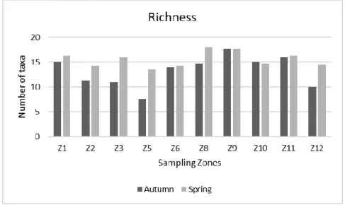
In terms of taxa richness, the number of families recorded in each zone can be observed in Figure 8. During the Autumn season, zones Z1, Z9, Z10 and Z11 represent the sampling areas with the most families (≥ 15) observed, while zone Z5 had the lowest number of taxa recorded during this time (n=7). Regarding the Spring sampling, the

richness recorded increased in most sampling zones when compared to the Autumn season.

Fig. 8 - Variation richness values at each sampling site, during the Autumn and Spring sampling campaigns.

To characterize the edaphic community of the BGP and its dynamic, Shannon Diversity Index (Figure 9) and Pielou Equitability Index (Figure 10), were calculated for each sampling zone in both sampling seasons. In ecological studies, most diversity values varied between 1.5 and 3.5, and rarely greater than 4.0 (Magurran, 2004; Kerkhoff, 2010). The highest recorded value of diversity in this study was observed in zone Z9 (H’=0.991) in the Spring sampling period, while the lowest value was observed in Z10 (H’=0.541) for the same sampling period. These values show that this study presented low diversity values (Magurran, 2004; Kerkhoff, 2010). In the Autumn period, the highest values of diversity were recorded at zones Z1 (H’=0.966) and Z11 (H’=0.965), while the lowest values were observed in zones Z10 (H’=0.612) and Z12 (H’=0.601). This latter, largely due to the high number of Springtails presented in these areas in comparison to other arthropod groups. In the Spring sampling campaign, an increase in diversity can be observed for most sampling zones, with the highest diversity value observed in zone Z9 (H’=0.991), and the lowest diversity observed in zone Z10 (H’=0.541). In this zone, the situation may be explained by the soil parameters (ex: high values of organic matter content of 27.98%) and vegetation cover (ex: Hedera sp., see Table 1) recorded in this zone, with the Springtails comprising the majority of organisms found in this zone. The high values of organic matter observed in this zone, explains the presence of the organisms recorded in the area (Springtails, Beetles and Opiliones), decomposers of organic matter through its fragmentation.

Fig. 9 - Variation of the Shannon Diversity Index (Mean + SD) at each sampling site, during the Autumn and Spring sampling campaigns.

The Pielou’s Equitability Index varies between 0 and 1 (Beisel et al., 2003). The here-obtained results show almost values higher than 0.5. The maximum values recorded in Autumn was in zones Z1 (J’=0.831) and Z2 (J’=0.816) and the lowest values were observed in the zones Z3 (J’=0.513) and Z10 (J’=0.518). After analyzing both figures (9 and 10), a trend can be observed when a high diversity value occurred a high value of evenness was observed. This is meaning that the number of organisms of each species in each sampling zone is balanced, with no species standing out from each other in the distribution. Although this may be the case in the majority of sampling zones, it is not observed in zones Z3 and Z10. In these zones occurred a high abundance of Springtails resulting in lowest values of the Shannon Diversity and Pielou Equitability Indexes.

Fig. 10 - Variation of the Pielou Equitability Index (Mean + SD) at each sampling site, during the Autumn and Spring sampling campaigns.