2 Fractional delaylead of discrete-time signals

Introduction to fractional linear systems.

Part

zyxwvutsrqponmlkjihgfedcbaZYXWVUTSRQPONMLKJIHGFEDCBA

2:

Discrete-time case

zyxwvutsrqponmlkjihgfedcbaZYXWVUTSRQPONMLKJIHGFEDCBA

M.D.Ortigueira

zyxwvutsrqponmlkjihgfedcbaZYXWVUTSRQPONMLKJIHGFEDCBA

Abstract:

zyxwvutsrqponmlkjihgfedcbaZYXWVUTSRQPONMLKJIHGFEDCBA

In the paper, the class of discrete linear systems is enlarged with the inclusion of

discrete-time fractional linear systems. These are systems described by fractional difference equations and fractional frequency responses. It is shown how io compute the impulse response and transfer function. Fractal signals are introduced as output of special linear systems: fractional differaccumulators, systems that can be considered as having fractional poles or zeros. The concept of fractional differaccumulation is discussed, gencralising the notions of fractal and lif

noise, and introducing two kinds of fractional differaccumulated stochastic proccss: hyperbolic, resulting from fractional accumulation (similar to the continuous-time casc), and parabolic noise, resulting from fractional differencing.

1 Introduction

In a companion paper [ 11, we presented an introduction to

fractional continuous-time linear systems. Such systems may be suitable for modelling several signals and systems found in practice. However, there are other similar situa- tions where the continuous-time approach is not suitable; for example, in hydrology and economics there are time series with fractional characteristics that are not well fitted

by the usual ARMA models

zyxwvutsrqponmlkjihgfedcbaZYXWVUTSRQPONMLKJIHGFEDCBA

[ 2 ] . The results obtained for

continuous-time fractional systems have motivated us to consider the discrete-time counterpart. Although there are few current applications of fractional discrete-time systems, they are interesting and motivating cnough for the development of the theory of such systems. The so-

called fractional delay filter [3, 41 is a system for band- limited interpolation between samples and is used in communications, speech processing, music technology, and array processing. In communications, fractionally spaced equalisers [5] became very popular, due to their performance. Attempts have been made to use fractional discrete-time systems in control [6-81 and economics [2, 9, IO]. Here a combination of an ARMA model with a

fractional differencing has been used (see also [ l 11). These systems can be considered special cases of frac- tional discrete-time linear systems. In this paper, we present a generalisation of the usual theory to include these systems. Similarly to the situation verified previously [ 11, we find here that we are led to a formulation that looks like the usual formulation, leading to the impression that there is nothing new. However, that is not the case in practice, since to our knowledge there is no published work describing the systems we are considering here.

:i‘ IEE 2000

f E E Proceedngs onlinz

zyxwvutsrqponmlkjihgfedcbaZYXWVUTSRQPONMLKJIHGFEDCBA

no. 20000273

DOI: 10. I049/ip-vis:20000273 Paper received 13th September 1999

The author is with the Instittito Superior Tecnico and UNINOVA, Campus

da FCT da UNL, Quinta

zyxwvutsrqponmlkjihgfedcbaZYXWVUTSRQPONMLKJIHGFEDCBA

d a Torre 2825 - I14 Monte da Caparica, Portugal

and also with INESC, R. Alves Rcdol, 9, 2 ; , 1000 Lisbon, Portugal

[EE Pruc.-Vts. Imuge Signul Proces., @I. 147, No. 1, Feehruurv 2000

Usually discrete-time linear systems are described by difference equations, and characterised by their impulse responses and corresponding transfer functions and frequency responses. In the following we are concerned with the study of the linear systems described by fractional difference equations. These are similar to the usual, but admit non-integer delays or leads. For these equations we generalise the referred responses.

Wc begin by considering the definition of fractional delay and lead (‘dellead’). We use the unit delay [4] with a discrete-time Fourier transform (FT) equal to e’“’”, enabling us to generalise, again with the help of convolu- tion, the usual translation property of the discrete-time FT.

This, we define ‘dellead’ for signals with discrete-time FT. The next steps would lead us to try a similar definition concerning the dellead in the context of the Z transform (ZT). Unfortunately, there is no causal or anti-causal sequence with ZT equal to z‘(Iz/ # 1 and r g z ) . This important fact forces us to use another method: the Cauchy integrals. These are operators that perform a projection of a function defined on the unit circle over the regions outside (casual case) or inside (anti-causal case) thc unit circle. With these integrals we can treat the causal systems described by linear fractional difference equations, enabling us to define transfer function and impulsc response. The developed theory is suitable for obtaining the modified ZT from the ZT [ 121.

We present an introduction of the fractional delayilead (dellead). The treatment of the fractional delleads in the ZT context is carried out with the help of the Cauchy integrals, and examples are presented. We also study the linear systems described by fractional difference equations, and introduce the notions of fractional transfer function and impulse response. We use the partial fraction expansion, and treat the cases corresponding to rational and irrational delleads. Stability is also studied. The initial condition problem is discussed, and the results are used later, when we introduce a state-space formulation. Fractal signals [ 14, 151 are introduced as output of special linear systems: fractional differaccumulators, systems that can be consid- ered as having fractional poles or zeros. The concept of fractional differaccumulation is also discussed.

2 Fractional delay/lead of discrete-time signals

zyxwvutsrqponmlkjihgfedcbaZYXWVUTSRQPONMLKJIHGFEDCBA

we conclude that

zyxwvutsrqponmlkjihgfedcbaZYXWVUTSRQPONMLKJIHGFEDCBA

2. '1.

zyxwvutsrqponmlkjihgfedcbaZYXWVUTSRQPONMLKJIHGFEDCBA

Fractional delay/lead

In practical applications of discrete systems, mostly we deal with signals that are sampled versions of continuous- time band-limited signals. Normally, these signals are processed synchronously, in the sense that the time domain is the set of integer numbers for all of them. However, there are applications where this does not happen. We can process signals obtained by sampling continuous-time signals with the same sampling interval but in different instants of time, e.g. the so-called time- delayed processes [ 6 ] . On the other hand, in other applica-

tions, we may need to know the behaviour of a system between the sampling instants [ 121. The current application of multi-rate techniques allows the conversion of a signal sampled with a given sampling interval to another one with

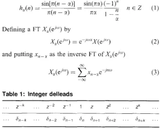
a different sampling interval. These considerations are intended to be a motivation for the theory we are going to develop. The notions of 'delay' and 'lead' are usually defined only for integer multiples of a given time interval. Essentially, and by analogy with fractional differintegra- tion, we intend to generalise these notions to allow for fractional delay and lead (dellead). In Table 1 we present a

relation between integer delleads and powers of

zyxwvutsrqponmlkjihgfedcbaZYXWVUTSRQPONMLKJIHGFEDCBA

z.

We intend to prolong the sequences to give sense to (5,,-,

(To make the theory similar to that developed for contin- uous-time systems, we use here the Kronecker

6

instead of Dirac d(t). To avoid confusion, we use the notation 6(')(t) to

represent the a-order differintegration of Dirac 6 ( t ) and

a,,

-,

to represent the fractional translation of the Kronecker 6,)

and z-". We assume

zyxwvutsrqponmlkjihgfedcbaZYXWVUTSRQPONMLKJIHGFEDCBA

x to be any non-integer real. If x i 0,

we have a fractional lead; if U.

zyxwvutsrqponmlkjihgfedcbaZYXWVUTSRQPONMLKJIHGFEDCBA

> 0, we have a fractional delay.

When

zyxwvutsrqponmlkjihgfedcbaZYXWVUTSRQPONMLKJIHGFEDCBA

a is integer, we fall into the usual scheme.

We are looking for sequences, ~3,-~: bilateral (with e-Ju" as FT) or causal, and anti-causal (with z-" as the Z-transform). For this, we have tried to compute the inversion integral using the theory of complex variable functions. The function z-' has a branch point at z=O. Any branch cut will cross the unit circle but will not serve to define two regions like IzIi 1 and 1z1> 1. Therefore, we

cannot impose causality by the choice of the branch cut, in contrast to the continuous-time case [14]. On the other hand, if a is not integer, z-" with IzI

#

1 does not have a

convergent MacLaurin or Laurent expansion, which implies that there is no causal nor anti-causal sequence with z-" as ZT. The bilateral case is very simple: it is enough to compute the inverse discrete-time Fourier trans- form, h,(n), of e-j"". It is readily computed and is given by

sin[n(n - a)] sin(nx) (- 1)"

n(n - x) 711 I - -

-

- _______ n E

z

(1)

h,(n) =

Defining a FT Xx(eJW) by

and putting x,-" as the inverse FT of Xx(eJ0)

cy:

-00

zyxwvutsrqponmlkjihgfedcbaZYXWVUTSRQPONMLKJIHGFEDCBA

Table 1: Integer delleads

. . . 2 - k . . . 2 - 2 2 - 1 1 z

zyxwvutsrqponmlkjihgfedcbaZYXWVUTSRQPONMLKJIHGFEDCBA

1 _ . .

zx

(note that this formula remains valid for any real x.)

Eqn. 3 defines the modified Fourier transform [12] that is a special case of the Zak transform [ 131 and generalises the translation property of the FT. Eqn. 4 (essentially the Shannon-Whitaker interpolation formula) is very impor- tant, since it states a relation between two signals x,, and

=x,+, defined in the sets Z and { nz;m = n

+

x, n E Z and

x E R } , respectively. Thus, we are relating two signals

defined over two time grids, obtained one from the other by a fractional translation (note that this formula remains valid for any real r ) . The relation in eqn. 4 is a convolution between x, and /z,(n), which can be considered as the impulse response of a reconstruction filter that is non- causal and IIR; a review of FIR and all-pass filter design techniques for bandlimited approximation of this filter is presented elsewhere [4], together with several applications. According to the properties of the convolution and to the fact that h,(rz) is square summable, it is enough that x,, is also square summable to guarantee that the series in eqn. 4 is convergent. Using Fourier transform theory, we can show that this relation remains valid if x,, is an absolutely summable signal.

With eqns. 2-4 we are ready to define fractional differ- ence equations and to introduce a frequency response for the systems represented by such equations.

According to the notation used in Table 1, we can substitute h,(n) for 6,,-,:

6,,-, = h,(n) if r non-integer (5) Thus, we can write eqn. 4 in the form

Dgx,, = x,-, = x,, x h,(n) = x,,

*

d,,_, ( 6 )

This is analogous to the differintegration of a continuous- time signal [ 11.

Continuing our sequence of thoughts, we look for the causal and anti-causal solutions for fractional delleads. We would like to generalise eqn. 2 for signals with ZT:

X J z ) = z P X ( z ) Iz/ > 1 or Iz/ < 1 _{( 7 )} This fact means that we were looking for the impulse response of a filter with transfer function equal to z" (it is interesting to note that X , ( z ) is the modified ZT [12]).

However, as previously concluded [ l ] , there is no such filter. Therefore, to obtain

X,(z),

we perform analytic continuations of a function g ( z ) defined on the unit circle

(z=ei"") to the region / z / > 1 (G+(z)) and 1z1 < 1 ( G - ( z ) ) ,

in such a way that their projections on the space corre- sponding to that circle satisfy eqn. 92 (see Appendix):

G+(z)

+

G - ( z ) = g ( z ) for /zI = 1 (8) The extrapolations are obtained through the use of the Cauchy's integrals (see Appendix), We obtain the ZT of the causal and anti-causal parts of a given signal, from its Fourier transform. As shown in the Appendix

and

g(w)

zyxwvutsrqponmlkjihgfedcbaZYXWVUTSRQPONMLKJIHGFEDCBA

‘ z

zyxwvutsrqponmlkjihgfedcbaZYXWVUTSRQPONMLKJIHGFEDCBA

. w-’

zyxwvutsrqponmlkjihgfedcbaZYXWVUTSRQPONMLKJIHGFEDCBA

G-(z) =

L /

dw

zyxwvutsrqponmlkjihgfedcbaZYXWVUTSRQPONMLKJIHGFEDCBA

2rcj w - z

zyxwvutsrqponmlkjihgfedcbaZYXWVUTSRQPONMLKJIHGFEDCBA

L is the integration path: the unit circle. In fact, let X(w) be

given by

zyxwvutsrqponmlkjihgfedcbaZYXWVUTSRQPONMLKJIHGFEDCBA

00

and

From eqn. 9 we obtain

30

X + ( Z ) = C x , , z - n

0

For the anti-causal case. the situation is similar:

x-

(z) = x,zpn

00

The use of eqns. 13 and 3 allows us to obtain

zyxwvutsrqponmlkjihgfedcbaZYXWVUTSRQPONMLKJIHGFEDCBA

oc 00

For the anti-causal case, the procedure is similar:

-00 -00

These results lead us to introduce formally the modified ZT by

This means that if a given signal has a ZT, it also has a modified ZT. However, there is no operator to allow us to

obtain directly the modified ZT from the ZT, or vice versu.

zyxwvutsrqponmlkjihgfedcbaZYXWVUTSRQPONMLKJIHGFEDCBA

3 Discrete-time fractional linear systems

3.

I

Difference fractional equations

In this Section, we generalise the concept of difference equation in order to consider non-integer delays or leads. Consider the linear time-invariant systems characterised by

a difference equation that adopts the general form Nil

r=O J=O

~ , D ” ~ y ( n ) = b,Dvix(n) n E Z (1 8) where D is the difference operator (delay) and the v, are the delays that, in the general case, are real numbers. This means that we made D’ny(t) =y(t - v,). According to our

considerations in Section 2 the relation D”lzn = z-”’zn

remains valid only for jz/ = 1; in this case, we obtain, easily

MJ

b,zY’J

This is a frequency response function. Again, according to our earlier considerations, we can obtain the transfer functions, corresponding to causal and anti-causal systems by using the Cauchy integrals for projecting H ( z ) in eqn. 19 defined on the unit circle outside and inside it. To obtain the impulse response, we must perform the inversion of the transfer function. As in the continuous-time case, in the following we consider that the v, are either rational numbers or are multiples of a common real, v. Eqns. 18 and 19 then adopt the format

N M

and

M

We use the term ‘fractional autoregressive moving average (FARMA) system’. In contrast to the continuous-time case, we must consider two situations; the general FARMA system and the particular (fractional MA - FMA). This

latter case is very easy to deal with, because H(eJW) is given by

f!4

H(eJif’) =

C

bnle-Jmwi’ (22)

m=O

we only have to use eqn. 9 to obtain H+(z). We have

nn

and

Thus, the impulse response is

M

n > O

m=O

If v = liq

I M l a l 0-1

zyxwvutsrqponmlkjihgfedcbaZYXWVUTSRQPONMLKJIHGFEDCBA

k=O I=O

The symbol

1.J

means integer part. If q = 1, we obtain the usual response corresponding to a FIR system.

Next we consider the general FARMA case. Without restrictions, we may assume that the fraction in eqn. 21 is proper. The computation of the impulse response follows steps similar to the continuous-time case.

( a ) Consider the function H(w), by substitution of w for z”. ( h ) The polynomial denominator in

H(w)

is the indicia1 polynomial or characteristic pseudo-polynomial. Perform the expansion of

H(w)

into partial fractions such as

(27)

1

F(w) =

(1 - a ‘ w - y

(c) Substitute back

zyxwvutsrqponmlkjihgfedcbaZYXWVUTSRQPONMLKJIHGFEDCBA

z" for

zyxwvutsrqponmlkjihgfedcbaZYXWVUTSRQPONMLKJIHGFEDCBA

MI to obtain

zyxwvutsrqponmlkjihgfedcbaZYXWVUTSRQPONMLKJIHGFEDCBA

H ( z ) expanded as a linear combination of fractions such as

(4

Compute the impulse responses corresponding to each

partial fraction.

( e ) Add the impulse responses.

These steps allow us to test the stability of fractional linear time-invariant discrete-time systems, according to how we obtain the impulse response. In fact, we have transformed the denominators in rational functions of M , ~ ' . The proper- ties of the response corresponding to each partial fraction depend on the poles, as in the non-fractional case. Thus, to test the stability of the fractional linear systems, we only

have to check if the poles are outside the unit circle.

zyxwvutsrqponmlkjihgfedcbaZYXWVUTSRQPONMLKJIHGFEDCBA

3.2 Partial fraction inversion

3.2.1 Rational case: We proceed to the inversion of the partial fraction (eqn. 28). Let us consider the case

where k = 1 and

zyxwvutsrqponmlkjihgfedcbaZYXWVUTSRQPONMLKJIHGFEDCBA

v = llq.

zyxwvutsrqponmlkjihgfedcbaZYXWVUTSRQPONMLKJIHGFEDCBA

The problem resumes to the

computation of the inverse ZT of

For v

zyxwvutsrqponmlkjihgfedcbaZYXWVUTSRQPONMLKJIHGFEDCBA

= we have

The procedure that is followed is almost identical to that used in the continuous-time case [ l ] and consists of transforming the partial fraction into another equivalent one:

i,- I

For the proof, it is enough to sum the numerator on the right-hand side. If la1 < 1, we can rewrite eqn. 31 in the form

We thus conclude that the inverse ZT of F+(z), f'(n), is given by

9-1 30

f ( n ) = a' Uqn26,,-,,l-j,, n

zyxwvutsrqponmlkjihgfedcbaZYXWVUTSRQPONMLKJIHGFEDCBA

1 0 (33)

i=O NI=O

It is interesting to note that this case can be obtained from eqn. 26 with M = 00 and setting b,,, an exponential

sequence. The result (eqn. 31) states that if 11 is rational, the general FARMA system has another equivalent description in terms of a transfer function with a rational denominator. In addition, eqns. 31 and 33 lead us to conclude that the computed impulse response is, in fact, a weighted average (a', i = 0 , . . . , q - 1, as weights) of 9

responses of a first-order system to impulses applied at - - i v ( i = O , . . . , q - 1).

In the k > 1 case, the convolution property can be used, or we can relate eqn. 28 with the ( k - 1)th derivative of 1/( 1 - a . z - " ) and use the differentiation property of

the FT.

74

3.2.2 Irrational case: Consider now the case corre- sponding to v as an irrational number. We manipulate eqn. 32 directly. Assume for now that ( U ( < 1. In this case, we have

Proceeding as in the previous case, we obtain

x

(35)

This is the discrete analogue to the Mittag-Leffler function

[l]. To test the coherence of this result, make 11 a rational number: = llq in eqn. 34. Now put n = 1 . q

+

i ( I = 0, 1, 2 , . .

.

; i = O , 2 , . . . , q - 1) in the summation symbol to

obtain

This leads to eqn. 32. With a similar substitution in eqn. 35, we are led to eqn. 33 again.

3.2.3 Practical example: The Unit delay operator has been studied previously [4], and several approaches to implement causal approximations for it proposed. Here, we propose an alternative based on the theory we have presented: the fractional linear prediction.

Let x ( n ) n E Z be a real stationary stochastic process, observed up to time n - 1, and let R,(k) be its autocorrela-

tion function. We define the Nth order d-step prediction at

12 - 1 + d ER) (in fact, if d < 0, we are making an

interpolation, not a prediction) by

,\

where U , (i = 1, . . . , N) are the coefficients of the d-step predictor (with d = 1, we obtain the usual one-step predic- tion). The predictor coefficients are chosen in order to minimise the prediction error power:

P , = E[(n(n - 1

+

d ) - 2(n - 1

+

d))'] ₍₃₈₎

Assuming that the correlation matrix has rank at least equal to

N,

the minimisation of the prediction error power (eqn. 38) is easily performed by differentiation of its right-hand side in order to all the a, (i = 1 , . . . , N), and leads to the following set of normal equations:

2 n j , R ( k - i) = -R(-k - d + 1) k = 1 , 2 , . . . ,

N

I = 1

(39)

whence we obtain the predictor coefficients. As an applica- tion example, we performed the computation of the predic- tor coefficients for x,, = cos(wOn). The predictor is given by and

X,+d = coS[oJo(n

+

d ) ] (41) as expected. It is a simple matter to implement this algorithm in a lattice form. In addition, the predictor coefficients can be adaptively computed.

4 Results on fractional systems

zyxwvutsrqponmlkjihgfedcbaZYXWVUTSRQPONMLKJIHGFEDCBA

4.

I

zyxwvutsrqponmlkjihgfedcbaZYXWVUTSRQPONMLKJIHGFEDCBA

Initial value problem

zyxwvutsrqponmlkjihgfedcbaZYXWVUTSRQPONMLKJIHGFEDCBA

In ordinary linear systems, either continuous-time or discrete-time, the insertion of the initial conditions when they are not zero is very simple, since the one-sided

Laplace and

zyxwvutsrqponmlkjihgfedcbaZYXWVUTSRQPONMLKJIHGFEDCBA

Z transforms make them appear explicitly.

The same happens with the fractional continuous-time systems [ I ] . However, this does not happen here, because, in general, the number of initial values is not finite. We do not consider the problem with all generality. We consider a simple case for insight into the solution of the state variable equations.

Assume a continuous-time difference equation:

x(t 1

zyxwvutsrqponmlkjihgfedcbaZYXWVUTSRQPONMLKJIHGFEDCBA

a ) = x ( t ) r > 0, t > 0 ₍₄₂₎

As known, the solution is the causal periodic repetition of a given initial function xo(t) defined in the interval [0, a [ .

Thus

x(t I na) = xo(t) t E [0, a[ and n = 0, I , 2,

. . .

(43) Consider a point to E [0, a [ . This point may be considered the origin of a sequence

t,, = to

+

na n = 1 , 2 ,

.

. . (44)

where x(t) assumes the same value, x(to). Let

zyxwvutsrqponmlkjihgfedcbaZYXWVUTSRQPONMLKJIHGFEDCBA

Tf a and

consider another sequence

zyxwvutsrqponmlkjihgfedcbaZYXWVUTSRQPONMLKJIHGFEDCBA

tkT = k . T T E R and k = 1 , 2 , . . . ₍₄₅₎ Consider the set of points belonging to both sequences. It is evident that, in gencral, their intersection is empty. A necessary and sufficient condition for non-empty intersec- tions is that to, T, and a are commensurate:

(46)

where p , q, and r are positive integers. In this case, for a

given integer k, there is one s E {0, 2 , . . . , p - 1 } such that

4 " n = k - + -

P P (47)

It is clear that the intersection set has infinite cardinality. In fact, if the pair (a, k ) verifies eqn. 47, all the pairs ( n

+

mq, k f m p ) with m = 0 , 1, 2 , . . . satisfy eqn. 46 and

x [ ( k

+

mp)T) assumes the constant value

zyxwvutsrqponmlkjihgfedcbaZYXWVUTSRQPONMLKJIHGFEDCBA

xo(r/p, a),

r E { 0 , 1 , 2 , . . . , p - 1 } . Considering all the values

assumed by r, we conclude that we will obtain a periodic

sequence x(kT) with period p . Therefore, we need p initial

conditions.

Let us proceed a little further by considering

x(t

+

x) = a ' x ( t ) (48)

Let X ( s ) be the unilateral Laplace transform of x(t). Apply

it to eqn. 48. After some easy manipulation, we obtain

1'6

x(z)e-"dz

1 - ue-w Re(s) > 0 (49)

X ( s ) =

If la1 e 1 and x(t) = x O ( t ) for t E [0, a [ ,

m

X ( s ) = ~ u n e - ' n a . xo(z)e-"dz Re(s) > 0 ( 5 0 )

n=O

.c

leading to

x(t) = unx,(t - na) t E [nx, ( n

+

I)a[ and n = 1 , 2 , . . . (51)

We conclude that this situation is similar to the previous one, but now the replications of the initial value no(s/p. r )

are weighted by a". Putting t = n r

+

co, r with 0 5 co < 1, it becomes

x[nr

+

E o . % ] = unx"[c0.a] n = 1 , 2 , . . . (52) and from eqn. 46,

x[np /q . T

+

r / q . TI = u"xo[r/q . TI

( 5 3 )

The integer

zyxwvutsrqponmlkjihgfedcbaZYXWVUTSRQPONMLKJIHGFEDCBA

Y' must be chosen in order to lead to an integer

value for the expression

O ( r c p ; n = l , 2 , . . .

k = n p / 4

+

r l q (54) Denote by rk the sequence of residuals obtained by divid- ing k . 4 by p . This sequence is periodic with period p . On

the other hand, when

IC

is increased by p , n is incremented

by q . Thus

x [ ( k + p ) . T ] = u"x(k T ) (55)

The Z transform gives

P- 1

x(i T ) P

X ( z ) = _{1 - aY .z-P} (56) where the initial values x(i. T ) belong to the set {xo(r. T ) ,

0 5 r c p } . The order of appearance depends on p and 4. For example, assume that p = 4 and q = 7 and, for simpli- city,

T =

1. In this case, x(l)=xo(3/7), x(2)=xo(2/7), x(3)=xo(1/7), and x(4)=x0(0). From eqn. 51 and making t = k - T, we obtain

kT E [nx, ( n

+

l ) a [ and k = 1 , 2 , . . .

x ( k T ) = uixo([)

(57)

where [ is the residual of the division of kT by x. Of course, n is the quotient: n = L/cT/aj. If Tir is not rational, the

sequence

zyxwvutsrqponmlkjihgfedcbaZYXWVUTSRQPONMLKJIHGFEDCBA

rk defined above is aperiodic, and so we need an

infinite number of initial values to define x(k ~ r ) for

k = l , 2, . . .

4.2 State variable representation

The state-space representation of a fractional linear system described by eqn. 20 is readily obtained and can be represented by

s(k

+

a ) = A s ( k ) I B x ( k ) y ( k ) = Cs(k)

+

D x ( k )

(58)

(59) and

where s ( t ) is the state vector. We do not perform the computation of the solution of eqns. 58 and 59, only to solve the homogeneous equation

s(k

+

a ) = A . s ( k ) ( 6 0 ) Assume that A is a non-singular matrix. According to Section 4.1, it is not hard to show that the solution for eqn. 60 is easily obtained from eqn. 56. However, that result is not compatible with the state variable formulation. We must have only one initial state. To avoid the problem, we have to assume that all the initial conditions are equal to

7 5

a given value,

zyxwvutsrqponmlkjihgfedcbaZYXWVUTSRQPONMLKJIHGFEDCBA

so. In this case, the solution of eqn. 60 is

given by

zyxwvutsrqponmlkjihgfedcbaZYXWVUTSRQPONMLKJIHGFEDCBA

~ ( k ) = @ ( k , 0 ) ~ ( 0 ) k > 0 (61) where, again, n is equal to LkTlr] and s(0) is a vector with all the components equal to a given constant, so.

As in the ordinary case, we have a state transition operator, given by

@(k, 0) = Ak

zyxwvutsrqponmlkjihgfedcbaZYXWVUTSRQPONMLKJIHGFEDCBA

k > 0 (62) This seems to suggest that, in the time-variant case, the

state transition operator must be given by

n

@(k, 0) = n ; l ( i ) ( k > 0) (63)

zyxwvutsrqponmlkjihgfedcbaZYXWVUTSRQPONMLKJIHGFEDCBA

i= 1

We do not pursue the study of this operator. However, we point out that it is not very difficult to see that, in general and according to the results of Section 4.1, it does not satisfy the semi-group property enjoyed by the ordinary state transition operator.

Having solved the homogeneous equation (eqn. 60), we are going to solve eqn. 58, under null initial conditions. This is readily done by the use of the theory developed in Sections 2.1 (eqns. 8 to 10) and 3.2 (eqn. 19). From eqn. 58 we obtain

[eJWuI - A I S ( ~ ~ ’ ) = B . x ( e J m ) ₍₆₄₎

Assuming that the determinant of A is less than one, we

can write

zyxwvutsrqponmlkjihgfedcbaZYXWVUTSRQPONMLKJIHGFEDCBA

cc

,qeiy

=

CA”

. ~ , ~ - i d n + l ) r . x(eic!i) ₍₆₅₎

zyxwvutsrqponmlkjihgfedcbaZYXWVUTSRQPONMLKJIHGFEDCBA

n=O

With the help of the Cauchy integrals (Section 2.1), we obtain

oc

s ( k ) =

C A n

. B.x[k - (n

+

l ) ~ ] k 2 0 (66) This shows that, to compute the state at instant t = kT, in addition to the current input value, we must know all the past values at instants t = kT - ( n

+

1)aT Note that these

values are computed from all the values of the input at t = kT with k = 0, 1, . . . , 00, unless we can use the algo-

rithm proposed in Section 4.1.

n=O

zyxwvutsrqponmlkjihgfedcbaZYXWVUTSRQPONMLKJIHGFEDCBA

5

zyxwvutsrqponmlkjihgfedcbaZYXWVUTSRQPONMLKJIHGFEDCBA

Fractional order pole or zero

In Section 3, we studied fractional linear systems having transfer functions with expansions in partial fractions with the general format (eqn. 28). As shown if v = l / q , with q a

positive integer, these fractions can be transformed into others with a non-fractional denominator. Thus, eqn. 28

corresponds to a fraction with a k-order pole. Now we generalise these results by introducing the notions of

fractional order pole, and similarly fractional order zero. In terms of systems, we consider systems with transfer functions

(67) corresponding to a v-order zero if v > 0, and to a v-order pole if v < 0. At a first glance, we would say that these systems are useless. However, the special case obtained by putting a = 1 in eqn. 67 is very important. It may be called the differaccumulator; fractional differencer if 1’ > 0, and accumulator (or integrator) if v < 0. These terms have been used in fractal modelling [ 14, 151 and 1 lfnoise [ 16, 171. In

H ( z ) = (1 - a.z-1)”

16

economics and hydrology [2, 9-1 11, a combination of an ARMA system and a differaccumulator has been used to model some experimental signals. The difference equation corresponding to eqn. 67 can be described by a fractional order difference equation:

(1 - a . D)’y,, = x,,

zyxwvutsrqponmlkjihgfedcbaZYXWVUTSRQPONMLKJIHGFEDCBA

or y,, = (1 - a . D)”s, (68) where D is the unit delay operator. The corresponding

impulse response is obtained from the coefficients of the binomial series. Note only that, for 111>

I N I

The corresponding impulse response is

The series is absolutely and uniformly convergent for

IzI> l a / . Essentially, eqn. 67 corresponds to the general- isation of the notions of finite difference { U = 1 and v = n } , (1 - z - ’ ) ~ and of accumulation { a = 1 and 11 = - n } (1 - z - ’ ) - ’ ~ . Alternatively, we can obtain another expres-

sion by using

This means that the system with transfer function

H(z) = (1 - a .z- I ) ” can be considered as an infinite order AR or MA system. This is a very singular and interesting case. We are interested in the special case when a = 1, fractional differencing ( v 0) or fractional accumulation (11 < 0).

Regarding the stability of the system ( I - Z - ’)’, we can say that

(i) if I: is a negative integer, it is unstable in general, except

the case when = - 1 (accumulator): in this situation. the

system is wide-sense stable.

(ii) if 1’ is a positive integer, it is a FIR, and so it is always

stable in every sense.

(iii) according to results presented elsewhere [ 181, the series

.

.

:

C

lhlll converges for every 1, > 0, but not for

0, the system will be stable in any sense; if

- 1 < v < 0, the system will be wide-sense stable, since the impulse response goes slowly to zero, h,,

< 0: if 1’

c n

-’-’:

and

(73)

where c is a positive constant, h,, RZ c . n-‘- ‘.

We conclude that if

11~1

< 1, the system is at least wide- sense stable and has two wide-sense stable representations (MA or AR).

As before, we define the fractional (discrete-time) stochastic process as the output of a fractional system excited by stationary white noise. Let h(k) be the impulse response of the system. Therefore, a fractional stochastic process is

n(k) = h ( k )

*

M(k) ₍₇₄₎

where

zyxwvutsrqponmlkjihgfedcbaZYXWVUTSRQPONMLKJIHGFEDCBA

n(k) is a stationary white noise with variance g2. We

define, as usual, the autocorrelation function and power

spectral density (spectrum) by

zyxwvutsrqponmlkjihgfedcbaZYXWVUTSRQPONMLKJIHGFEDCBA

DT

(75)

i=O

and

S,T(e'o')

zyxwvutsrqponmlkjihgfedcbaZYXWVUTSRQPONMLKJIHGFEDCBA

= o2

zyxwvutsrqponmlkjihgfedcbaZYXWVUTSRQPONMLKJIHGFEDCBA

.

IH(e'"')12 (76)

According to eqn. 7 4 , we define an a-order fractionally diffcraccumulated noise as the output of the system with impulse response given by eqn. 7 0 , with a = 1 , when the input is stationary white noise.

The computation of its autocorrelation function is slightly complex. Eqns. 7 0 and 75 allow us to obtain the autocorrelation function. Inserting eqn. 70 into eqn. 75, we obtain

or

Let us introduce the Gauss hypergeometric function [ 181:

where c

#

0 , - 1 , - 2 , . . . and ( u ) ~ is the Pochhammer

symbol: ( u ) ~ x u . (U

+

l ) ( a

+

2 ) . . . (U

+

k - 1). The series

in eqn. 79 is convergent for IzI 5 1, if c - a - h z 0 :

~ F , ( U , h; c; Z)

if 0 < h < c and larg(1 - z)I< n,

zyxwvutsrqponmlkjihgfedcbaZYXWVUTSRQPONMLKJIHGFEDCBA

that function can be

represented by the Euler integral As

and attending to

zyxwvutsrqponmlkjihgfedcbaZYXWVUTSRQPONMLKJIHGFEDCBA

(i

+

k ) !

zyxwvutsrqponmlkjihgfedcbaZYXWVUTSRQPONMLKJIHGFEDCBA

= (i

+

₍₈₂₎

and

( - x ) , + ~ = ( - ~ ) ~ ( - a

+

i)k

zyxwvutsrqponmlkjihgfedcbaZYXWVUTSRQPONMLKJIHGFEDCBA

(83)

we obtain

R,(k) = ~ ~ ( - 1 ) ~ .

C)

. ,F,(a, - E

+

k ; k

+

1; 1) k

>

0

(84)

Hosking [2] makes a distinction between long-term ( a < 0 )

and short-term ('x > 0 ) persistent processes, because when

x < 0 the impulse response goes very slowly to zero, contrary to the a > 0 case. Note that the systems we are dealing with are the discrete-time analogue of the differ- integrator in the continuous-time case. We have a differ- encer in the a > 0 case and an accumulator in the a < 0

case.

E E Pi-oc.-ViJ h u g e Signal Proce.s.s., 161. 147, No. I , Februury 2000

We define the spectrum by

s(ej"') = o2 . lim (1 - z-')"(1 - z)" ₍₈₅₎

(86) (87)

z+eJ"'

g 2 ,

I

1 - e-JLl 2"

I

- -

= o2 . [2 . sin(w/2)12?

If M > 0, the spectrum is graphically similar to a parabola. We use the term parabolic noise for the corresponding stochastic process. If a < 0, we follow Hosking's consid- erations to use the term hyperbolic noise, for the corre- sponding stochastic process, and it may be considered a

fractional Brownian process, since it is generated by 'integrating' white noise. Stochastic processes of this type are the discrete-time analogue to the continuous- time lif'noise, since near the origin S(w) is proportional to ( o ~ ~ . We can show that the first difference of a hyperbolic noise is a parabolic noise. Using the relation [ 181

after some simple manipulations we obtain

leading to the power of the process:

r ( i

+

2 4

+

1>12

P, = o2

if 1 + 2 a > 0 or a - 1/2. This means that, only for those

values, we may be led to a stationary stochastic process. If

la1 < 1/2, x(n) is simultaneously stationary and invertible [ 2 ] . If a = - 1/2, the process has an infinite power and can

be considered wide-sense stationary. This case is the most similar to the continuous-time hyperbolic noise defined previously. Asymptotically, the autocorrelation function given by eqn 89 is proportional to k-1-2y, again showing hyperbolic bchaviour. If a is positive, it goes quickly to zero, showing that the process is a short-term persistent process [2]. I f a is negative, it is the reverse situation; it is a

long-term persistent process.

An interesting result [6] refers to the partial autocorrela- tion function (reflection coefficient sequence). Its recursive computation with the usual Levinson-Durbin algorithm leads to

C, =

--SI

E + k k = 1 , 2 , .

. .

and la1 < 1/2 (91)

This is an interesting result: these processes are similar to

zyxwvutsrqponmlkjihgfedcbaZYXWVUTSRQPONMLKJIHGFEDCBA

MA processes, in the sense of the similarity of the behaviours of the reflection coefficients. As seen, while the autocorrelation function is asymptotically proportional to k-1-27 , the partial autocorrelation is proportional to k - ' , independently of a.

6

zyxwvutsrqponmlkjihgfedcbaZYXWVUTSRQPONMLKJIHGFEDCBA

Conclusions

In this paper, we have presented a class of linear systems: the fractional discrete-time systems. For the definitions of such systems, we have introduced the definitions of 'frac- tional delay' and 'lead'. These definitions have allowed us to present an approach that is very similar to that used in the study of the ordinary linear systems; we were led to the notions of 'fiactional impulse' and 'frequency responses'. We have shown how to compute them and to test the stability that is similar to the usual systems. The problem

of the initial conditions has also been discussed and a state variable formulation for the fractional linear time-invariant systems has been presented.

We defined the fractal stationary stochastic process as

the output of a stable linear system, with the transfer function characterised by having a fractional pole or zero

at

zyxwvutsrqponmlkjihgfedcbaZYXWVUTSRQPONMLKJIHGFEDCBA

z = 1. We have discussed the concept of fractional differaccumulation, generalising the notions of ‘fractal’

and ‘llf noise’, and introduced two kinds of fraction!lly differaccumulated stochastic process: hyperbolic (similar

to the continuous-time case) and parabolic noises.

zyxwvutsrqponmlkjihgfedcbaZYXWVUTSRQPONMLKJIHGFEDCBA

7

1

2

3

zyxwvutsrqponmlkjihgfedcbaZYXWVUTSRQPONMLKJIHGFEDCBA

4

5

zyxwvutsrqponmlkjihgfedcbaZYXWVUTSRQPONMLKJIHGFEDCBA

6

7

8

9

zyxwvutsrqponmlkjihgfedcbaZYXWVUTSRQPONMLKJIHGFEDCBA

References

ORTIGUEIRA, M.D.: ‘Introduction to fractional signal processing Part

1 :

zyxwvutsrqponmlkjihgfedcbaZYXWVUTSRQPONMLKJIHGFEDCBA

Continuous-time systems’,

zyxwvutsrqponmlkjihgfedcbaZYXWVUTSRQPONMLKJIHGFEDCBA

IEE Proc. Vis., Image Sigrml Pi-ocess.,

2000, 147, pp. 62-70

HOSKING, J.R.M.: ‘Fractional differencing’, Biometrik, 198 I ,

zyxwvutsrqponmlkjihgfedcbaZYXWVUTSRQPONMLKJIHGFEDCBA

68, (l),

pp, 165-176

HERMANOWICZ, E., ROJEWSKI, M., CAIN, G.D., and TARC- ZYNSKI: ‘Special discrete-timc filters having fractional delay’, Sigriul

Process., 1998, 67,,,pp. 279-289

LAAKSO, T.I., VALIMAKI, V , KALJALAINEN, M., and LAINE,

U.K.: ‘Splitting the unit delay’, IEEE Signcil

zyxwvutsrqponmlkjihgfedcbaZYXWVUTSRQPONMLKJIHGFEDCBA

Process. Mug., 1996, pp.

30-60

TREICHLER, J.R.. FIJALKOW, I., and JOHNSON. C.R. Jr: ‘Fraction- ally spaced equalizers: how long should they really be?’, IEEE Sigiiul

Process. Mug., 1996, pp. 65-81

DE PAOK, A.M., and O’MALLEY, M.J.: ‘The zero-order hold equiva- lent transfer function for a time-delaved process’, _~. hit. J Control, 1995,

61, (3), pp. 657-665

MACHADO, J.A.T.: ‘Analysis and design of fractional-order digital control systems’, SAMS, 1997, 27, pp. 107-122

MACHADO, J.A.T., and AZENHA, A.: ‘Positiodforce fractional control of mcchanical manitonlators’. Proceedinrs 1998 5th Int. Work- shop on Aclvunced Motion donfr.ol, Coimbra, Po&gal, pp. 2 16-22 1

CRATO, N.: ‘Recent I-escarch on fractional noise in economic time series’. Proccedings 3rd CEMAPRE Conference, May 199 1, Lisbon, ISEG, pp. 353-370

10 CRATO, N.: ‘Long memory time series models: a revicw’. Proceedings 3rd CEMAPRE Confcreuce, May 1991, Lisbon, ISEG, pp. 371-390

1 I DERICHE, M., and TEWFIK, A.H.: ‘Signal modelling with filtcrcd discretc fractional noise processes’, IEEE Tmns Signul Pmces.~., 1993, 12 JURY, E.I.: ‘Theory and application ofthe Z-transform method’ (Robert

E. Krieger Publishing Co., Huntington, Ne\v York)

13 JANSSEN, A.J.E.M.: ‘The Zak transform: a signal transfoini for sampled time-continnous signals’, Pl7d@S J Res., 1988, 43, pp. 23-69

14 MANDELBROT, B.B.: ‘The fractal gcometiy ofnature’ (W. H. Freeman and Company, New York, 1983)

15 MANDELBROT, B.B., and VAN NESS, J.W.: ‘The fractional brownian motions, fractional noises and applications’, S f A 4 Rev., 1968, 10, (4)

16 VAN DER ZIEL, A.: ‘Unified presentation of llf’noise in electronic devices: fundamental llf’noise sources’, Proc. fEEE, 1988, 7 6 , pp. 2 3 3 ~ - 258

41, (9)

17 KESHNER, M.S.: ‘l/fNoise’, Proc. IEEE, 1982, 70, pp. 212-218

18 SAMKO, S.G., KILBAS, A.A., and MARICHEV, 0.1.: ‘Fractional integrals and derivatives - theory and application’ (Gordon and Breach Science Publishers, 1987)

8 Appendix: Cauchy problem

Let L be the open unit circle {z:z = eJ“’, w E [ - 71,

zyxwvutsrqponmlkjihgfedcbaZYXWVUTSRQPONMLKJIHGFEDCBA

n[}. This circle decomposes the C plane into two regions: the interior

C, = {z: IzI< 1 ) and the exterior C, = {z:IzI > 1 ) .

De$nition 1

We define the Cauchy problem as consisting of the deter-

mination of two functions G- and C+, defined and

continuous over C, U L and C, U L , respectively, analytic

inside their domain, and satisfying

G-(z)

+

G+(z) = g ( z ) Vz E L (92)

We can consider C - and G+ as extrapolations of g ( z ) for the interior and exterior of the unit circle.

Definition 2

The integrals of the type

(93)

where L is an integration path (closed or not), are called Cauchy integrals.

If g ( w ) is a continuous function on L , G*(z) is analytic i n C - L a n d G + ( z ) + O w h e n z + 30.

The solution to the Cauchy problem is given by the Cauchy integral (eqn. 93), where the sign & is chosen according to the region of analyticity, C, or C;. This means that we obtain two functions that may be considered as unilateral Z-transforms. However, the solution is not unique. In fact, if A is a constant, the pair G-- (z) - A

and G+(z) + A also constitutes a solution for the problem.

For our purposes, the value of A must be determined

according to the initial value theorem. Assume that g(w),

zyxwvutsrqponmlkjihgfedcbaZYXWVUTSRQPONMLKJIHGFEDCBA

MJ =e””, is the FT of a given signal x,,. The solution to the problem is

1

.I’

g(M’) ‘ w-1

C+(Z) = - dw

2nj 1 - v i r 1

g ( w )

.

z . 1.1.-’ dw

G-(z) = -

By a process of analytic continuation, the function g ( z )