UNIVERSIDADE FEDERAL DE SÃO CARLOS CENTRO DE CIÊNCIAS BIOLÓGICAS E DA SAÚDE
PROGRAMA DE PÓS-GRADUAÇÃO EM ECOLOGIA E RECURSOS NATURAIS
Flávia Gomes de Mello
How short-term variation influence the relative importance of environmental
and spatial factors associated to anuran dissimilarity composition
CENTRO DE CIÊNCIAS BIOLÓGICAS E DA SAÚDE
PROGRAMA DE PÓS-GRADUAÇÃO EM ECOLOGIA E RECURSOS NATURAIS
Flávia Gomes de Mello
How short-term variation influence the relative importance of environmental
and spatial factors associated to anuran dissimilarity composition
Dissertação apresentada ao Programa de Pós-Graduação em Ecologia e Recursos Naturais da Universidade Federal de São Carlos como parte dos requisitos para obtenção do título de Mestre em Ecologia e Recursos Naturais.
Orientação: Profº Dr. Fernando Rodrigues da Silva
Ao meu orientador, Prof. Dr. Fernando Rodrigues da Silva, por quem carrego profunda admiração e respeito. Agradeço pela confiança, pela enorme paciência de sempre, pelos esclarecimentos e ensinamentos sobre ecologia, área que hoje me sinto apaixonada, e por despertar e manter vivo em mim o difícil porém gratificante caminho para a vida acadêmica.
Ao meu colega de pós-graduação e amigo - pessoa de enorme competência e humildade - Ronildo Benício, por me incentivar, ajudar e estar presente sem hesitar, em todas as vezes em que precisei.
Ao Caio, por ter sido o companheiro que fomentou em mim todas as ideias e anseios a respeito de iniciar e depois de continuar meus estudos dentro da Biologia, desde a minha entrada na graduação até o ingresso no mestrado.
À minha Mãe Lucimar, não só por sempre me apoiar em minhas escolhas, sofrer ou se alegrar junto a mim, mas acima de tudo por compreender com afeto minha enorme ausência em tantos períodos difíceis da sua vida- e ainda não só nos difíceis - como também nos momentos simbólicos, como nossas caminhadas pelo centro da cidade, companhia no preparo das refeições, nas saídas com o Raví, nas horas de conversas sobre política ou sobre qualquer banalidade, e claro nas suas tão adoradas maratonas de séries boas! Todos esses pequenos momentos que valorizo muito e dos quais estive totalmente ausente nesse período. Obrigada!
À minha sobrinha Bibia, por ser minha alegria, me presentear com seu sorriso lindo e por sempre dividir comigo toda a sua leveza nos finais dos meus dias desgastantes.
Aos meus irmãos e meu pai por me incentivarem e acreditarem no meu potencial, demonstrando respeito e admiração por mim e minha pesquisa.
Às minhas amadas amigas Aline e Roseli, companheiras de desespero, angústias e incertezas - mas sempre e finalmente companheiras de risos e alívios não só da vida acadêmica mas de todo o resto. E a todos os companheiros da graduação, com quem caminhei através das maravilhas do mundo da Biologia.
A todos os meus amigos, antigos e recentes, por ouvirem horas e horas de entusiasmo ou lamúrias na mesa do bar e ainda assim me quererem sempre por perto.
Ao Gui, por conseguir me trazer paz, leveza e confiança nessa reta final.
À Coordenação do Pessoal de Nível Superior CAPES, por me conceder auxílio financeiro, sem o qual não seria possível iniciar meu mestrado.
Este trabalho segue as exigências do Regimento Interno do Programa de Pós-Graduação em
Ecologia e Recursos Naturais (PPGERN) da Universidade Federal de São Carlos – UFSCAR (http://www.ppgern.ufscar.br/). A dissertação foi redigida no formato de artigo científico para
apreciação no periódico Plos One ISSN: 1932-6203. Contudo, realizamos algumas alterações em relação as normas descritas pela Plos One que julgamos melhorar a apresentação da dissertação. São elas: i) acrescentamos ao artigo um resumo redigido em português; e ii)
Sumário
Resumo... 2
Abstract ... 4
Introduction ... 5
Material and Methods ... 7
Study area and sampling... 7
Environmental variables ... 8
Community dissimilarity ... 8
Relative importance of environmental and spatial factors ... 9
Results ... 10
Community dissimilarity ... 10
Relative importance of environmental and spatial factors ... 10
Discussion ... 11
Conclusions ... 14
References ... 15
Figures ... 22
Tables ... 27
Resumo
Compreender os processos que originam os padrões na composição de espécies e a variação
na biodiversidade através do espaço tem sido um dos principais tópicos estudados dentro da teoria
de metacomunidades. Contudo, a maioria dos trabalhos utilizaram dados “fixos” das comunidades e
poucos estudos examinaram a importância de incluir variabilidade temporal nas análises. Neste
estudo, nós avaliamos a distribuição da diversidade beta na composição de comunidades de anuros
ao longo de três anos e considerando todo o período de estudo em diferentes escalas espaciais na
Mata Atlântica brasileira: i) sete comunidades distribuídas na região costeira; ii) sete comunidades
distribuídas na região do interior; e iii) todas as comunidades juntas. Nós particionamos a
diversidade beta total nos componentes substituição de espécies e aninhamento, e depois, utilizamos
a partição de variância para explorar a importância relativa dos fatores espaciais e ambientais
relacionados com a variação na distribuição da composição de espécies de anuros ao longo dos
anos. A substituição de espécies foi o componente predominante da diversidade beta de anuros. Nós
também observamos que os valores médios dos componentes da diversidade beta diminuíram
quando a composição de espécies foi analisada considerando o período total de estudo e
aumentaram com o aumento da extensão espacial. Além disso, nossos resultados indicam que a
composição de espécies de anuros na Mata Atlântica são dinâmicas no tempo e espaço, e os fatores
explicando a distribuição dos componentes substituição de espécies e aninhamento são dependentes
do ano de amostragem e da extensão espacial. Portanto, estudos de metacomunidades que não
consideram mudanças temporais e espaciais devem ser cuidadosos com respeito as generalidades de
suas conclusões biológicas.
Palavras-chave: montagem de comunidades, aninhamento, substituição de espécies, diversidade
How short-term variation influence the relative importance of environmental and
1
spatial factors associated to anuran dissimilarity composition
2
3
4
Flávia G. de Mello1*, Fernando R. da Silva2
5
6
7
8
1 Programa de Pós-Graduação em Ecologia e Recursos Naturais, Universidade Federal de São
9
Carlos, São Carlos, SP, Brazil
10 11
2 Laboratório de Ecologia Teórica: Integrando Tempo, Biologia e Espaço (LET.IT.BE),
12
Departamento de Ciências Ambientais, Universidade Federal de São Carlos, Sorocaba, SP, Brazil
13 14
15
* Corresponding author
16
E-mail: flaviagmell@gmail.com
17
18
19
20
Abstract
28
Understanding the processes that create the patterns of species composition and biodiversity
29
variation across the space has been one of the main topics within the theory of metacommunities.
30
However, most studies rely on static snapshots of community data and few studies have examined
31
the importance of including temporal variability. Here, we examined beta diversity distribution of
32
anuran community composition through three years and considering the whole period of study at
33
different spatial extents in the Brazilian Atlantic Forest: i) seven inland communities; ii) seven
34
coastal communities; and iii) communities pooled together. We partitioned total beta diversity into
35
species replacement and nestedness-resultant components then we used variation partitioning to
36
explore the relative importance of environmental and spatial factors explaining the distribution of
37
anuran community changes over the years.Species replacement was the predominant component of
38
anuran beta diversity. We observed that average values of beta diversity components decrease when
39
species composition of whole period of study are pooled together and increase with increasing
40
spatial extent. Furthermore, our results indicate that Brazilian Atlantic Forest anuran community
41
compositions are dynamic in space and time, and the factors explaining the distribution of species
42
replacement and nestedness-resultant are dependent of the sampling year and spatial extent. Thus,
43
metacommunity studies that do not evaluate different spatial and temporal changes should be
44
cautious about the generality of their biological conclusions.
45
46
Keywords: community assembly, nestedness-resultant, species replacement, temporal diversity,
47
variation partitioning
48
Introduction
50
Understanding the roles of dispersal, and niche-based (i.e. habitat filtering and biotic 51
interactions) and stochastic (i.e. random colonization-extinction) processes in shaping local 52
communities has been the main subject of metacommunity theory [1, 2, 3, 4]. In the last decades, 53
several empirical studies in metacommunity ecology have examined the relative importance of 54
space and environmental factors on the similarity of species composition among local sites relying 55
on static snapshots of community data [5, 6, 7]. The traditional absence of temporal variability on 56
community composition suggests that the structure of metacommunity remains constant through 57
time. However, richness and community composition change over time [8, 9, 10], and effects of 58
temporal variability in metacommunity theory remains little understood. For example, Fernandes et 59
al. (2014) [11] found that seasonal floodplain-fish metacommunity is structured by changes 60
between dispersal limitation and environmental filter through time. In contrast, Baselga et al. (2015) 61
[12] observed that land cover changes in agricultural landscape had little impact on temporal beta 62
diversity of bird assemblages. Considering that environmental and spatial processes are dependent 63
on the time of sampling, metacommunity studies based on single snapshots may differ about the 64
importance of different factors shaping local communities (e.g. patterns might be linked to 65
environmental factors at one year, but spatial factors at another year), especially when communities 66
are sampled across different periods. 67
Here, we simultaneously assessed spatial and short-term variation in anuran community 68
dissimilarity in the Brazilian Atlantic Forest. We partitioned total beta diversity into species 69
replacement and nestedness-resultant components [13, 14] through three years and considering the 70
whole period of study at different spatial extents: i) seven inland communities; ii) seven coastal 71
communities; and iii) communities pooled together. Evaluating local community dissimilarities at 72
different spatial extent, can be a tool to detect mechanisms structuring metacommunities that may 73
be interacting at local and/or regional scales [15, 16]. In this case, relationships between 74
and the range of environmental variation examined [17, 18, 19]. For example, patterns of 76
community dissimilarity associated with species interactions would be more likely to be explained 77
at smaller extent, whereas patterns of community dissimilarity associated with dispersal from 78
regional species pool would be more likely to be explained by larger extent [17, 18]. Furthermore, 79
evaluating species replacement and nestedness-resultant components of beta diversity can shed light 80
on the mechanistic underpinnings these patterns [20, 21, 22]. Compositional dissimilarity of two 81
local communities may reflect two antithetic phenomena, species turnover and species loss/gain 82
(Fig 1a) that when ignored might lead to inappropriate conclusions [13]. Therefore, these beta 83
diversity components should be disentangled in order to identify the underlying processes 84
responsible for observed patterns of community dissimilarity. 85
Brazilian Atlantic Forest, a global biodiversity hotspot [23], originally covered c. 1.3 million 86
km2, of which 16% remain not degraded by human activities [24]. This biome harbors as many as
87
600 amphibian species, of which c. 88% are endemic [25]. The great richness and endemism of 88
amphibians in this region are usually attributed to the strong climatic gradients and topographic 89
heterogeneity, and high turnover of amphibian species in space [21, 22], making it an ideal location 90
to assess the role of environmental and spatial factors on community dissimilarity at different 91
spatial extent. Based on this scenario, we asked if environmental and spatial factors correlated to
92
distribution of species replacement and nestedness-resultant components are similar over time or
93
dependent on the sampling year. Our first objective was to evaluate whether species replacement
94
and nestedness-resultant values are congruent through three years and considering the whole period
95
of study at different spatial extents (Fig 1b). Our second objective was to understand if ecological
96
processes such as environmental sorting and dispersal limitation are congruent through three years
97
and considering the whole period of study at different spatial extents (Fig 1c). Thus, if the ability of 98
correlative and mechanistic models to predict community dissimilarity change depending on the 99
specific year. We hope that this approach will help us to better understand the interaction of spatial
101
and temporal dynamics on the processes structuring community assembly.
102
103
Material and Methods
104
Study area and sampling
105
We used a short-term dataset with anuran incidence data from 14 protected areas in the
106
Brazilian Atlantic Forest (Fig 2). The sampling was carried out using standardize methods from
107
December to February for three consecutive years (2014 to 2017), totalizing 27 days in each
108
protected area. This period is the time of the year when most of annual rainfall occurs and most
109
anuran species are active. Six reproductive habitats were sampled in each area: two ponds, two
110
streams and two transects inside forest fragments. Surveys were carried out on streams and transects
111
inside forest fragments considering always the same extension of 100 m in all areas. Three sampling
112
methods were used to determine the anuran species composition in each reproductive habitat: i)
113
Survey at breeding site [26] - combining a visual and auditory search in the breeding habitats
114
between 19:00 hours and 24:00 hours; ii) survey of larvae with dipnetting - a long and wire hand net
115
(3 mm2 mesh size) was used along the margins of ponds and streams, sampling the available
116
microhabitats from 12.00 hours to 18.00 hours; and (iii) visual encounter [27] – two people walked
117
slowly for 30 minutes in trails inside the forest fragment, streams and around ponds looking at
118
microhabitats for individuals hidden under trunks, bromeliads, stones, branches, and leaf litter. The
119
combination of sampling methods increases the efficiency of recording anuran species in
120
communities [28].
121
There is general agreement that the regional species pool and the spatial extent are
122
fundamental issues influencing the processes involved in metacommunity assembly [4]. Thus, we
123
limited the areas sampled in this study at different spatial extent (Fig 2) and regional species pool
124
based on the biogeographic regions of anurans in the Brazilian Atlantic Forest [29]. These authors
125
split anuran species composition into four regions that are broadly congruent with the vegetation
formations of the Atlantic Forest: (1) Region 1, located in AtlanticForest inland areas, composed by
127
semideciduous forest and some areas of transition to the Cerrado; (2) Region 2 comprises mostly
128
the ombrophilous forest, located in the coastal Atlantic Forest in southeastern Brazil; (3) Region 3 is
129
mostly congruent with the Araucaria forest in southern Brazil; and (4) Region 4 encompasses the
130
northeastern Brazilian semideciduous and ombrophilous forests. Our study area comprises the most
131
southeastern region of the country, encompassing the Region 1 and 2 according to the work of
132
Vasconcelos et al (2014).
133
134
Environmental variables
135
We gathered monthly precipitation data (December, January and February) for each site
136
over the three sampled years (Table 1). For this, we used accumulated monthly precipitation
137
available in the online governmental platform of the Centro Integrado de Informações
138
Agrometereológicas (http://www.ciiagro.sp.gov.br/). When data were not available, we used the
139
precipitation values from the location closest to the protected area considering a maximum radius of
140
35 km. For statistical analysis, we considered, for each year separately, the sum of precipitation
141
over the three months (Table 2). In contrast, when the data were analyzed together, we used the
142
mean of precipitation over the three years (Table 2). We used Google Earth to obtain maximum
143
(MAEL) and minimum (MIEL) elevation for each protected area. Then, we calculated the
144
elevational range (difference between MAEL and MIEL) (Table 2).
145
146
Community dissimilarity
147
We calculate beta diversity between inland and coastal communities separately and after 148
all communities together. We analyze the results of each year and then check the congruence of the 149
results over the years.We used the additive partitioning approach proposed by Baselga (2010, 2012)
150
[13, 14], in which the Sorensen dissimilarity (βsor) index is decomposed into two additive
components: (1) the species replacement component (βsim), which measures the proportion of
152
unique species in two sites pooled together if both sites are equally rich; and (2) the
nestedness-153
resultant component (βsne), which measures how dissimilar the sites are due to a nested pattern.
154
We performed Linear mixed effect models to assess the distributions of βsor, βsim and βsne
155
values separately through time using pairwise distances as repeated measures. All analyzes were
156
performed using software R 3.4.3. [30] using 'betapart' [31] and 'nmle' [32] packages.
157
158
Relative importance of environmental and spatial factors
159
We used distance-based Moran’s Eigenvector Maps (dbMEMs) [33, 34] to describe 160
spatial structures. The eigenvectors of dbMEM are determined from a truncated geodesic distance 161
matrix calculated using the longest distance connecting two sites in a minimum spanning tree as a 162
threshold. Then, we used a forward selection procedure with double stopping criteria [35] to only 163
select environmental variables and dbMEMs that significantly explained the variance in the species 164
composition matrix [36] considering inland and coastal sites and the sites pooled together 165
separately. 166
We assess the relative importance of environmental and spatial factors (dbMEMs) using 167
variation partitioning [37]. This approach partitions the total percentage of variation into unique and 168
shared contributions of the sets of predictors. The total variation in the pairwise beta diversity 169
components was divided into four fractions: i) the variation explained purely by space; ii) the 170
variation explained purely by environmental variables; iii) the shared variation explained by 171
environmental and space; and iv) unexplained variation (residual). We performed partial 172
redundancy analysis with 999 Monte Carlo permutations to test significance of variation explained 173
purely by environmental and spatial factors [35]. 174
All analyzes were performed using software R 3.4.3. [30] using 'vegan' [38] and
175
'adespatial' [39] packages.
Results
177
Community dissimilarity
178
We found that independently of sampling year or spatial extent, βsim was the predominant
179
component of the beta diversity (Fig 3). Furthermore, average values of dissimilarity species
180
composition were different considering inland sites (Fβsor3,60= 10.18, p < 0.001; Fβsim3,60 = 5.23, p =
181
0.002; Fβsne3,60= 4.11, p = 0.01; Fig 3B), coastal sites (Fβsor3,60= 36.39, p < 0.001; Fβsim3,60 = 37.73, p
182
< 0.001; Fβsne3,60= 1.34, p = 0.26; Fig 3B) and sites pooled together (Fβsor3,270= 34.37, p < 0.001;
183
Fβsim3,270 = 36.05, p < 0.001; Fβsne3,270= 9.49, p < 0.001; Fig 3C). We also found that independent of
184
the spatial extent, values of dissimilarity species composition considering years pooled together are
185
lower than values of dissimilarity species composition from separated years (Fig 3).
186
187
Relative importance of environmental and spatial factors
188
The strength of relative importance of the environmental and spatial factors through time 189
was depended on the sampling year and spatial extent (Fig 4). For inland sites, 190
the total dissimilarity (βsor) between communities was explained by environmental variables and 191
space only in the second year (Fig 4A). During the first year species replacement (βsim) was not 192
associated with environmental factors, but in the other years, there were association with these 193
factors (Fig 4B). Still for the inland communities, the nestedness component (βsne) was explained 194
by the environment and space only in the first year sampled (Fig 4C). However, when we analyze 195
the data of the three years together we do not observe a power of explanation of both environmental 196
and spatial factors (Fig. 4A-C). 197
For coastal communities in general, environmental variables had little or no explanatory 198
power for each year separately and from the years together (Fig 4D-F). The spatial factors not 199
explained the dissimilarity between communities in the second year, but instead explained from 200
(Fig 4D-F). When we consider the communities pooled together, we notice a decrease in the 202
explanation power of the environmental variables and an increase in the power of explanation of the 203
space on the beta diversity. In this case we still observe a variation in the force of explanation of the 204
space between the years (Fig 4G-I). Furthermore, we found that increasing the spatial extent the 205
values of residual for βsor and βsim decrease (Fig 4G-H). In addition, the nestedness component
206
(βsne) was explained by the environment and space only in the first and second years (Fig 4I). 207
208
Discussion
209
We observed a temporal and spatial variation independently of the beta diversity component.
210
The correlation of environmental and spatial variables with dissimilarity distributions was
211
dependent on the year sampled. According to Dornelas et al. (2012) [40], among the main factors to 212
which temporal changes in biodiversity can be attributed are systemic changes (reflection of a non-213
stationary system where there are long-term changes in ecological directions), which may be 214
anthropogenic or natural processes. Although many studies focus on temporal variation in
215
biological communities caused by anthropogenic disturbances [8], these variations also occur
216
frequently in natural environments due for example to colonization of new spaces, adaptive
217
radiations and annihilation of a community [40]. However, each time observation can arise from the
218
combination of deterministic and stochastic effects, and the processes involved in these changes
219
depend on the components of biodiversity being studied and on the spatial and temporal extent of
220
the data [40].
221
Although many works performed with vertebrate and temporal beta diversity have found
222
important results, most of them used a long-term scale [41, 12]. Here we use a short-term scale,
223
since amphibians in addition to having a shorter life cycle compared to birds or mammals for
224
example, are easily affected by periodic climatic conditions, extinguishing or propitiating the
225
increase of certain species or populations in the localities. Environmental variability occurs over
226
time because of environmental fluctuations, and these changes may cause temporary microhabitats
and thus contribute to a difference in species composition of the community in different periods [42,
228
43]. Here, for the inland communities, the environmental variables had greater explanatory power
229
explaining beta diversity distribution than in the second and third year of sampling that were drier
230
years for some communities compared to the first year sampled (Table 1). For coastal communities
231
that are in the wettest portion of the biome, we observed no influence of the environmental
232
variables explaining the dissimilarity between them for the first and third year of sampling, which
233
were the driest years. However, for the second year, where accumulated monthly precipitation was
234
higher, rainfall was more important to explain the dissimilarity found among communities than
235
space. When we consider the two regions together we lose the explanatory power of the
236
environmental variables and increase the force of explanation of the space. Recently, França et al. 237
(2017) [44] evaluated the temporal fluctuations in the occurrence and abundance of amphibian 238
species in a portion of the Amazon rainforest, they found that greater species richness and 239
abundance occur during rainy periods, however, they pointed out that species may react differently 240
while some are sensitive to fluctuations, others do not seem to respond easily or do not reduce their 241
abundances at potentially unfavorable times. Similarly, Davis et al. (2017) [45] verified that the
242
persistence and colonization of amphibian metacommunities in the Florida’s northwestduring a
six-243
year period was affected differently by environmental disturbances with some amphibians being
244
more sensitive to drought and others more sensitive to periods of high precipitation. Péntek et al.
245
(2016) [46] evaluating amphibians in Central Europe in different periods of rain verified a change
246
between years in the relative role of spatial and local processes. All these studies revealed a
247
complex connection of spatial and temporal factors with the structuring the communities. Thereby,
248
determining the periods of fluctuations that species compositions of sites may vary over time and
249
the patterns associated with them is of extreme importance, considering that possible
250
misunderstandings can be generated in the absence of these temporal observations [47, 46, 45].
251
We observed that evaluating all communities together the explanatory power of the
252
environmental variables decreases while the explanation of the space increases. This phenomenon
can be explained by a consequent amplification of the biogeographic processes, which can result in
254
stronger limits on the dispersion of individuals, making communities even more differentiated [17,
255
48, 49, 50]. One of the potential determinants of beta diversity is the size of the species pool, which
256
may vary depending on the region considered [51]. Currently we find a climatic variation between
257
the different phytophysiognomies of the Atlantic Forest, passing through very humid
258
Ombrophylous Dense forests near the coast and portions of dry Semideciduous Seasonal forest that
259
contact the domain of Cerrado, found more in the interior [24, 29].This heterogeneity is the result
260
of different historical and biogeographic processes that have occurred over time. Biogeographic
261
processes such as climatic oscillations and periods of glaciations during the Pleistocene and
262
consequent reduction of wetlands (model of refuges) may have generated different evolutionary
263
histories among the species in these regions [52]. Other hypotheses are based on geological
264
changes, such as the isolation of mountains and the emergence of rivers as physical barriers to
265
contribute to the processes of speciation of these sites. However, environmental gradients and
266
altitudinal differences could also have served as ecotones for favoring divergent selection [52].
267
Therefore, these processes were important to determine the difference in species composition
268
among the communities found today in the different physiognomies of the Atlantic Forest.
269
We found that species replacement was the predominant component of anuran beta
270
diversity. Previous studies have already revealed species replacement as the main component of
271
beta diversity distributions [53, 21]. The environmental heterogeneity and the climatic differences
272
found in the coastal and interior regions, such as climate and altitude, are significant, mainly when
273
considered microhabitats used by the anurans. In coastal communities it was found greater species
274
richness as well as higher elevational range compared to the inland communities. These factors may
275
result in an increase of beta diversity values due to physiological limitations of anurans along
276
climate gradients. For example, amphibians have high physiological sensitivity and wide
277
morphological and behavioral diversity, adapted to different climatic and environmental conditions.
278
These characteristics resulted in different reproductive strategies and the use of specific
microhabitats during the development and life cycle of this group [54]. However, the variation in
280
the composition of the communities over time may be associated not only to the deterministic
281
processes, such as environmental and climatic changes, which can act as filters for different species
282
(niche perspective), but also in combination to stochastic processes, such as extinction and species
283
colonization, where the distribution of the species locally takes place randomly in response to a
284
possible ecological equivalence between them (neutral dynamic) [1, 55, 56, 57, 58]. Therefore, we
285
must consider a broader view in determining which processes act in the dissimilarity between
286
metacommunities, demonstrating for example that the combination of stochastic and deterministic
287
processes can often provide a better explanation for the distribution of species in a community [59].
288
289
Conclusions
290
Our results indicate that Brazilian Atlantic Forest anuran community compositions are
291
dynamic in space and time, and the factors explaining the distribution of species replacement and
292
nestedness-resultant are dependent of the sampling year and spatial extent. Taken together, these
293
results emphasize the importance of including spatial and temporal variables to questions which
294
seek to understand patterns, processes and elements that drive the complex dynamics of factors
295
associated with dissimilarity among ecological communities. Thus, metacommunity studies that do
296
not evaluate different spatial and temporal changes should be cautious about the generality of their
297
biological conclusions.
298
299
300
References
302
1. Leibold MA, Holyoak M, Mouquet N, Amarasekare P, Chase JM, Hoopes MF, Holt RD,
303
Shurin JB, Law R, Tilman D, Loreau M, Gonzalez A. The metacommunity concept: a
304
framework for multi-scale community ecology. Ecol Lett. 2004; 7: 601–613.
305
2. Holyoak, M,Leibold MA, Holt RD. Metacommunities: spatial dynamics and ecological
306
communities. Chicago: Univ of Chicago Press; 2005.
307
3. Chase JM, Myers JA. Disentangling the importance of ecological niches from stochastic
308
processes across scales. Philos Trans R Soc B: Biol Sci. 2011; 366: 2351–2363. 309
4. Leibold MA, Chase JM. Metacommunity ecology. 1st ed. Princeton University Press; 2018.
310
5. Cottenie K. Integrating environmental and spatial processes in ecological community
311
analysis. Ecol. Lett. 2005; 8: 1175–1182.
312
6. Soininen J. A quantitative analysis of species sorting across organisms and ecosystems.
313
Ecology. 2014; 95: 12, 3284 – 3292.
314
7. Soininen J. Spatial structure in ecological communities – a quantitative analysis. Oikos.
315
2016; 125, 2, 160 – 166.
316
8. Magurran AE, Dornelas M. Biological diversity in a changing world Introduction. Philos
317
Trans R Soc B Biol Sci. 2010; 365: 3593-3597.
318
9. Dornelas M, Gotelli JN, McGill B, Shimadzu H, Moyes F, Sievers C, et al. Assemblage time
319
series reveal biodiversity change but not systematic loss. Science. 2014; 344: 296-299.
320
10.Sarremejane R, Cañedo-Arguelles M, Prat N, Mykra H, Muotka T, Bonada N. Do
321
metacommunities vary trough time? Intermittent rivers as model systems. J Biogeogr. 2017;
322
44, 12: 2752- 2763.
323
11.Fernandes IM, Henriques-Silva R, Penha J, Zuanon J, Peres-Neto PR. Spatiotemporal
324
dynamics in a seasonal metacommunity structure is predictable: The case of floodplain-fish
325
communities. Ecography. 2014; 37: 464–475.
12.Baselga A, Bonthoux S, Balent G. Temporal beta diversity of bird assemblages in
327
agricultural landscapes: land cover change vs. stochastic processes. PLoS ONE. 2015; 10(5):
328
e0127913. pmid:26010153.
329
13.Baselga A. Partitioning the turnover and nestedness components of beta diversity. Glob Ecol
330
Biogeogr. 2010; 19: 134–143.
331
14.Baselga A. The relationship between species replacement, dissimilarity derived from
332
nestedness, and nestedness. Glob Ecol Biogeogr. 2012; 21: 1223–1232.
333
15.Ricklefs RE. Community diversity: relative roles of local and regional processes. Science.
334
1987; 235: 167–171.
335
16.Hille Ris Lambers J, Adler PB, Harpole WS, Levine JM, Mayfield MM. Rethinking
336
community assembly through the lens of coexistence theory. Annu Rev Ecol Syst. 2012; 43:
337
227–248.
338
17.Nekola JC, White PS. The distance decay of similarity in biogeography and ecology. J
339
Biogeogr. 1999; 26: 867–878.
340
18.Tuomisto H, Ruokolainen K, Yli-Halla M. Dispersal, environment, and floristic variation of
341
Western Amazonian Forest. Science. 2003; 299: 241–244.
342
19.McGill BJ, Dornelas M, Gotelli NJ, Magurran AE. Fifteen forms of biodiversity trend in the
343
Anthropocene. Trends Ecol Evol. 2015; 30: 104–113.
344
20.Svenning JC, Fløjgaard C, Baselga A. Climate, history and neutrality as drivers of mammal
345
beta diversity in Europe: insights from multiscale deconstruction. J Anim Ecol. 2011; 80:
346
393–402.
347
21.da Silva FR, Almeida-Neto M, Arena MVN. Amphibian beta diversity in the Brazilian
348
Atlantic Forest: Contrasting the roles of historical events and contemporary conditions at
349
different scales spatial. PLoS One. 2014; 9, e109642.
22.Melchior LG, Rossa-Feres DC, da Silva FR. Evaluating multiple spatial scales to understand
351
the distribution of anuran beta diversity in the Brazilian Atlantic Forest. Ecol Evol. 2017;
352
7:2403–2413.
353
23.Mittermeier AR, Fonseca GAB, Rylands AB, Brandon K. A brief history of biodiversity
354
conservation in Brazil. Conserv Biol. 2005; 19: 601 – 607.
355
24.Ribeiro MC, Metzger JP, Martenser AC, Ponzoni FJ, Hirota MM. The Brazilian Atlantic
356
Forest: how much is left, and howis the remaining forest distributed? Implications for
357
conservation. Biol Cons. 2009; 142: 1141–1153.
358
25.Haddad CFB, Toledo LF, Prado CPA, Loebmann D, Gasparini JL. Guide to the amphibians
359
of the Atlantic Forest: Diversity and biology. São Paulo, Brazil: Anolis Books; 2013.
360
26.Scott Jr. NJ, Woodward BD. Standard techniques for inventory and monitoring: Surveys at
361
Breeding Sites. Pp.118–125, inHeyer, W.R. et al. (Eds.), Measuring and Monitoring
362
Biological Diversity: Standard Methods for Amphibians. Smithsonian Institution Press;
363
1994.
364
27.Crump ML, Scott Jr. NJ. Visual encounter surveys. In: Heyer, W. R. et al. (ed.), Measuring
365
and monitoring biological diversity: standard methods for amphibians. Smithsonian
366
Institution Press; 1994. pp. 84–92.
367
28.da Silva FR. Evaluation of survey methods for sampling anuran species richness in the
368
Neotropics. SAJH. 2010; 5: 212–220.
369
29.Vasconcelos TS, Prado VHM, da Silva FR, Haddad CFB. Biogeographic distribution
370
patterns and their correlates in the diverse frog fauna of the Atlantic Forest hotspot. PLoS
371
One. 2014; 9, e104130.
372
30.R Development Core Team. R: A language and environment for statistical computing,
373
reference index ver. 3.4.3. - R Foundation for Statistical Computing, 2014;
374
<http://www.Rproject.org/>.
31.Baselga A. Partitioning abundance-based multiple-site dissimilarity into components:
376
balanced variation in abundance and abundance gradients. Methods Ecol Evol. 2017; 8:
377
799-808.
378
32.Pinheiro J, Bates D, DebRoy S, Sarkar D, R Core Team.nlme: Linear and Nonlinear Mixed
379
Effects Models. R package version. 2017; 3.1-137,
https://CRAN.R-380
project.org/package=nlme.
381
33.Dray S, Legendre P, Peres-Neto PR. Spatial modelling: a comprehensive framework for
382
principal coordinate analysis of neighbor matrices (PCNM). Ecological Modelling in press;
383
2006.
384
34.Dray S, Legendre P, Peres-Neto PR. Community ecology in the age of multivariate
385
multiscale spatial analysis. Ecol Monogr. 2012; 82: 257-275.
386
35.Legendre P, Legendre L. Numerical Ecology. Elsevier Science BV; 2012.
387
36.Blanchet FG, Legendre P, Borcard D. Forward selection of explanatory variables. Ecology.
388
2008; 89: 2623–2632
389
37.Borcard D, Legendre P, Drapeau P. Partialling out the spatial component of ecological
390
variation. Ecology. 1992; 73: 1045–1055.
391
38.Oksanen J, Blanchet FG, Friendly M, Kindt R, Legendre P, McGlin D, et al. vegan:
392
Community Ecology Package. - R package ver. 2.4-3, 2017
<https://CRAN.R-393
project.org/package=vegan>.
394
39.Dray S, Blanchet G, Borcard D, Guenard G, Jombart T, Larocque G, et al. – R package
395
‘adespatial’, 2017.
396
40.Dornelas M, Magurran AE, Bucklund ST, Chao A, Chazdon RL, Colwell RK, et al. 397
Quantifying temporal change in biodiversity: challenges and opportunities. Proc. R. Sci B.
398
2012; 280: 20121931.
41.Wojciechowski J, Heino J, Bini, L, Padial A. Temporal variation in phytoplankton beta
400
diversity patterns and metacommunity structures across subtropical reservoirs. Freshwater
401
Biology. 2017; 62: 10.1111/fwb.12899.
402
42.White EP, Ernest S, Adler PB, Hurlbert AH, Lyons SK. Integrating spatial and temporal
403
approaches to understanding species richness. Philos Trans R Soc Lond B Biol
404
Sci. 2010; 365: 3633–3643.
405
43.Ochoa-Ochoa LM, Whittaker R. Spatial and temporal variation in amphibian
406
metacommunity structure in Chiapas, Mexico. J Trop Ecol. 2014; 30: 537–549.
407
44.França DPF, Freita MA, Ramalho WP, Bernarde OS. Local diversity and influence of
408
seasonality on amphibians and reptiles assemblages in the Reserva Extrativista Chico
409
Mendes, Acre, Brazil. Iheringia, Sér. Zool. 2017; 107:
410
e2017023. http://dx.doi.org/10.1590/1678-4766e2017023
411
45.Davis CL, Miller DAW, Walls SC, Barichivich WJ, Riley JW, Brown ME. Species
412
interactions and the effects of climate variability on a wetland amphibian metacommunity.
413
Ecol Appl. 2017; 27: 285–296.
414
46.Péntek AL, Vad CF, Zsuga K, Horváth Z. Metacommunity dynamics of amphibians in years
415
with differing rainfall. Aquatic Ecol. 2016; 1573-5125.
416
47.Padial AA, Ceschin F, Declerck SAJ, De Meester L, Bonecker CC, Lansac-Têha FA, et
417
al. Dispersal ability determines the role of environmental, spatial and temporal drivers of
418
metacommunity structure. PLoS One. 2014; 9, e111227
419
48.Hubbell SP. The unified neutral theory of biodiversity and biogeography. Princeton:
420
Princeton Univ. Press; 2001.
421
49.Soininen J, Heino J, Wang J. A meta-analysis of nestedness and turnover components of
422
beta diversity across organisms and ecosystems. Glob Ecol Biogeogr. 2017; 1-14.
423
50.Logue JB, Mouquet N, Peter H, Hillebrand H. Empirical approaches to metacommunities: a
424
review and comparison with theory. Trends Ecol Evol. 2011;26: 482–491 2.
51.Kraft N, Comita LS, Chase JM, Sanders NJ, Swenson NG, Crist TO, Stegen JC, Vellend M,
426
Boyle B, Anderson MJ, Cornell HV, Davies KF, Freestone AL, Inouye BD, Harrison SP,
427
Myers JA. Disentangling the drivers of beta diversity along latitudinal and elevational
428
gradients. Science. 2011; 333: 755–175.
429
52.Carnaval AC, Moritz C. Historical climate modelling predicts patterns of current
430
biodiversity in the Brazilian Atlantic forest. J. Biogeogr. 2008; 35: 1187-1201.
431
53.Tisseuil C, Leprieur F, Grenouillet G, Vrac M, Lek S. Projected impacts of climate change
432
on spatio-temporal patterns of freshwater fish beta diversity: A deconstructing approach.
433
Glob Ecol Biogeogr. 2012; 21: 1213–1222.
434
54.Pombal JRP, Haddad CFB. Estratégias e modos reprodutivos de anuros (Amphibia) em uma
435
poça permanente na Serra de Paranapiacaba, Sudeste do Brasil. Pap. Avul. Zool. 2005; 45:
436
15, 201 – 2013.
437
55.Chase JM. Stochastic community assembly causes higher biodiversity in more productive
438
environments. Science. 2010; 328: 1388–1391.
439
56.Diniz‐Filho JAF, Siqueira T, Padial AA, Rangel TF, Landeiro VL, Bini LM. Spatial
440
autocorrelation analysis allows disentangling the balance between neutral and niche
441
processes in metacommunities. Oikos. 2012; 121: 201–210.
442
57.Prado VHM, Rossa-Feres DDC. The influence of niche and neutral processes on a
443
neotropical anuran metacommunity. Austral Ecol. 2014; 39(5): 540-547.
444
58.Si X, Ding P. Revealing beta-diversity patterns of breeding bird and lizard communities on
445
inundated land-bridge islands by separating the turnover and nestedness components. PLoS
446
One. 2015; 10: e01227692.
447
59.Roque FO, Guimaraes EA, Ribeiro MC, Escarpinati SC, Suriano MT, Siqueira T. The
448
taxonomic distinctness of macroinvertebrate communities of Atlantic Forest streams cannot
449
be predicted by landscape and climate variables, but traditional biodiversity indices
450
can. Brazil. Journ. of Biol. 2014; 74: 991-999.
Suporting Information
452
453
S1 Table. Species composition in the first year sampled. List of anuran species recorded from
454
December 2014 to February 2015on 14 protected areas in the Brazilian Atlantic Forest.
455
S2 Table.Species composition in the second year sampled. List of anuran species recorded from
456
December 2015 to February 2016 on 14 protected areas in the Brazilian Atlantic Forest.
457
S3 Table. Species composition in the third year sampled. List of anuran species recorded on 14
458
protected areas in the Brazilian Atlantic Forest from December 2016 to February 2017.
459
S4 Table. Species composition for the three years sampled. List of anuran species recorded on
460
14 protected areas in the Brazilian Atlantic Forest considering three years pooled together.
461
462
463
464
465
466
467
468
469
470
471
472
Figures
474 475
476
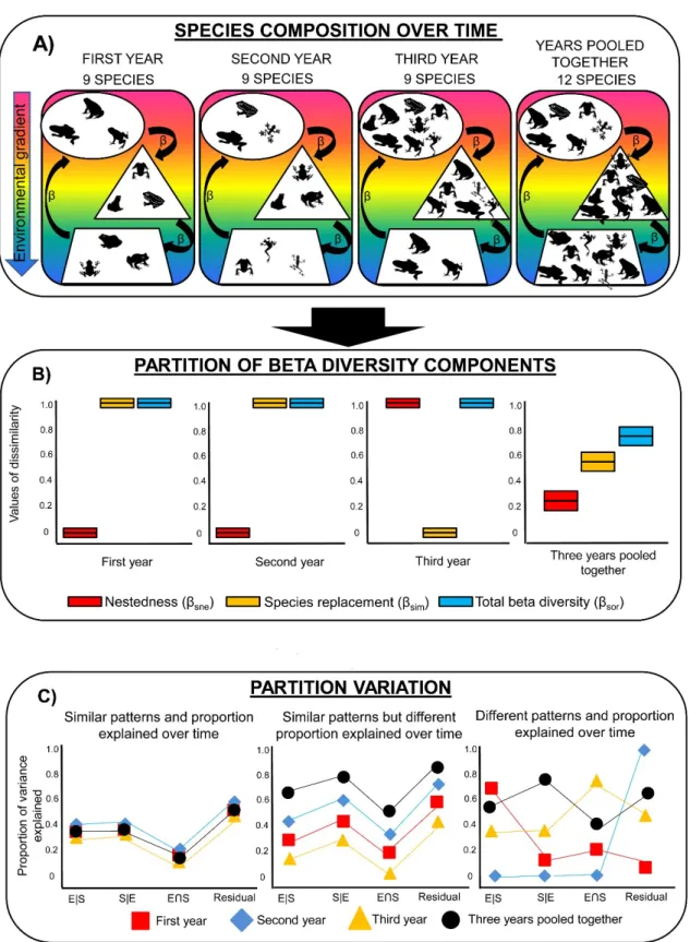
Fig 1. Representative scheme of the approach used in this study. A) Hypothetical distribution of
477
anuran species in three different communities (white geometric figures) over three consecutive
478
years and considering the three years pooled together. Colors represent illustrative environmental
gradient influencing anuran species composition. B) Four scenarios showing the partition of total
480
beta diversity (βsor) into species replacement (βsim), and nestedness (βsne) components. In the first
481
two scenarios, even the species composition being different between them, we observe high values
482
of turnover indicating that βsim is the main component describing the variation in species
483
composition along the environmental gradient. On the other hand, in the third year, βsne is the main
484
component explaining the variation in species composition among communities. In this case, we
485
observe that some anurans species are lost along the environment gradient, but there is no species
486
replacement between communities. In the fourth year, there is a balance on the importance of βsim
487
and βsne describing the variation in species composition among communities. C) Three scenarios
488
showingthe relative importance of environmental and spatial factors explaining variation in anuran
489
community composition. In the first scenario, there is congruence about factors and proportion of
490
variance explained over the years. In the second scenario, there is congruence about factors but the
491
proportion of variance explained is dependent on the year. In the third scenario, factors and
492
proportion of variance explained are different among years. E|S = variation explained purely by
493
environment; S|E = variation explained purely by space; E∩S = spatially structured environment; 494
Residual = variation not explained by the variables used in the study.
495
496
497
499
Fig 2. Study area. Map showing the state of São Paulo highlighted in Brazil (left) and the protected
500
areas where we carried out field surveys (right) over three consecutive years. Blue dots represent
501
the protected areas within inland spatial extent while orange dots represent the protected areas
502
within coastal spatial extent. Acronyms and consecutive names of protected areas plotted on the
503
map: EEAS – Estação Ecológica de Assis, EECA – Estação Ecológica de Caetetus, EEIT – Estação
504
Ecológica de Itirapina, EEJA – Estação Ecológica de Jataí, EESB – Estação Ecológica de Santa
505
Bárbara, FEENA – Floresta Edmundo Navarro, PEVA – Parque Estadual Vassununga, EECB –
506
Parque Estadual Carlos Botelho, EEJI – Estação Ecológica Juréia Itatins, PECU – Parque Estadual
507
da Serra do Mar Curucutu, PEJU – Parque Estadual Jurupará, PESV – Parque Estadual da Serra do
508
Mar Santa Virgínia, PETAR – Parque Estadual Turístico do Alto Ribeira, PESB – Parque Estadual
509
da Serra do Mar São Sebastião.
510
514
Fig 3. Results for community dissimilarity. Boxplot showing the decomposition of pairwise
515
Sorensen dissimilarity (βsor) into species replacement (βsim) and nestedness (βsne) components over
516
time considering (A) small spatial extent with seven inland protected areas; (B) small spatial extent
517
with seven coastal protected areas; and (C) broad spatial extent with all protected areas together.
518
The horizontal black line and box show the median and 50% quartiles, respectively, and the error
519
bars display the range of the data. Similar letters indicate significant difference (p < .05) between
520
average dissimilarity values over time.
522
Fig 4. Results for relative importance of environmental and spatial factors. Proportion of the
523
variation of Sorensen dissimilarity (βsor), species replacement (βsim) and nestedness (βsne)
524
components of beta diversity explained by correlations with environmental and spatial factors over
525
time. (A-C) small spatial extent with seven inland protected areas; (D-F) small spatial extent with
526
seven coastal protected areas; and (G-I) broad spatial extent with all protected areas pooled
527
together. E|S = variation explained purely by environment; S|E = variation explained purely by
528
space; E∩S = spatially structured environment; Residual = variation not explained by the variables 529
used in the study.
530
531
532
Tables
534 535
Table 1: Accumulated precipitation data (millimeter – mm) for each protected area considering the three months (December , January and February) in which the anuran samplings were carried out along the three sampled years. Data obtained from online governmental platform of the Centro Integrado de Informações Agrometereológicas (http://www.ciiagro.sp.gov.br/).
Sites Accumulated monthly precipitation by period (mm)
Dec.
2014 2015 Jan. 2015 Feb. 2015 Dec. 2016 Jan. 2016 Feb. 2016 Dec. 2017 Jan. 2017 Feb. Inland
EEAS 187 211 201 160 261 187 166 215 139
EECA 230 191 197 211 292 285 216 265 181
EEIT 248 89 49 50 328 16 174 326 42
EEJA 186 120 239 79 97 13 0 2 1
EESB 134 117 164 77 210 67 134 288 147
FEENA 134 157 235 124 272 109 175 294 76
PEVA 186 120 239 79 97 13 0 2 1
Coastal
EECB 254 125 195 106 295 204 1 0 27
EEJI 197 174 118 167 301 328 0 4 0
PECU 160 183 250 227 257 199 0 4 0
PEJU 149 3 1 242 178 83 123 270 113
PESV 107 105 275 191 199 0,2 117 0 27
PETAR 188 96 235 140 235 428 128 217 109
PESB 256 222 310 95 139 98 37 387 61
536
537
538
539
540
541
542
543
Table 2. Precipitation (millimeter – mm) and altitude data for each protected area considered in this study. Precipitation was determined considering the sum of the three months (December , January and February) in which the anuran samplings were carried out and the mean of the three years for each protected area. Precipitation data were obtained from online governmental platform of the Centro Integrado de Informações Agrometereológicas (http://www.ciiagro.sp.gov.br/). Altitude data were obtained from Google Earth ( https://www.google.com.br/intl/pt-BR/earth/).
Sites Environmental Variables
Sum of precipitation over the three months (mm) Altitude data First
year Second year Third year the years Mean of Maximum altitude Minimum altitude Altitude range
Inland
EEAS 599 608 521 576 601 450 151
EECA 618 787 662 689 703 452 251
EEIT 386 394 542 441 810 510 300
EEJA 545 189 3 246 788 530 258
EESB 416 355 569 447 740 530 210
FEENA 527 505 545 526 792 598 194
PEVA 545 189 3 246 788 528 260
Coastal
EECB 574 605 27 402 916 178 738
EEJI 489 796 4 430 1030 0 1030
PECU 593 683 4 427 901 40 861
PEJU 152 503 506 387 920 430 490
PESV 487 391 145 341 1030 600 430
PETAR 520 803 454 592 1001 120 881
Appendix
545SUPPLEMENTARY INFORMATION
546How short-term variation influence the relative importance of environmental and spatial factors associated to anuran dissimilarity
547
composition
548
Flávia G. de Mello, Fernando R. da Silva 549
Plos One 550
551
S1 Table. Species composition in the first year sampled. List of anuran species recorded from December 2014 to February 2015on 14 protected 552
areas in the Brazilian Atlantic Forest. 553
Species Inland sites Coastal sites
EEAS EECA EEIT EEJA EESB FEENA PEVA EECB EEJI PECU PEJU PESV PETAR PESB
Adenomera marmorata 0 0 0 0 0 0 0 1 1 1 1 1 1 1
Adenomera sp. 0 0 0 0 0 0 0 0 0 0 0 0 0 1
Aparasphenodon bokermanni 0 0 0 0 0 0 0 0 0 0 0 0 1 0
Aplastodiscus albofrenatus 0 0 0 0 0 0 0 0 0 0 0 1 0 1
Aplastodiscus albosignatus 0 0 0 0 0 0 0 0 0 0 0 0 0 1
Aplastodiscus perviridis 0 0 0 0 1 0 0 0 0 0 0 0 0 0
Bokermannohyla circumdata 0 0 0 0 0 0 0 0 0 1 1 1 0 0
Bokermannohyla astartea 0 0 0 0 0 0 0 1 0 0 0 0 0 0
Bokermannohyla hylax 0 0 0 0 0 0 0 1 0 1 1 1 1 1
Brachycephalus pitanga 0 0 0 0 0 0 0 0 0 0 0 1 0 0
Chiasmocleis leucosticta 0 0 0 0 0 0 0 0 0 0 0 0 0 1
Crossodactylus caramaschii 0 1 0 0 0 0 0 1 0 0 0 0 0 0
Cycloramphus boraceiensis 0 0 0 0 0 0 0 0 0 0 0 0 0 1
Cycloramphus eleutherodactylus 0 0 0 0 0 0 0 0 0 0 0 0 1 0
Dendrophryniscus brevipolicatus 0 0 0 0 0 0 0 1 0 1 0 1 0 1
Dendropsophus berthalutzae 0 0 0 0 0 0 0 0 1 0 0 0 0 1
Dendropsophus elegans 0 0 0 0 0 0 0 1 1 1 1 0 0 0
Dendropsophus elianeae 0 1 1 0 1 0 0 0 0 0 0 0 0 0
Dendropsophus giesleri 0 0 0 0 0 0 0 1 0 0 0 0 0 0
Dendropsophus jimi 0 0 1 0 1 0 0 0 0 0 0 0 0 0
Dendropsophus microps 0 0 0 0 0 0 0 1 1 0 1 1 1 0
Dendropsophus minutus 1 1 1 1 1 1 0 1 1 1 1 1 1 0
Dendropsophus nanus 1 1 0 1 1 1 1 0 0 0 0 0 0 0
Dendropsophus seniculus 0 0 0 0 0 0 0 0 0 0 0 0 0 1
Dendropsophus werneri 0 0 0 0 0 0 0 0 1 0 1 0 1 0
Elachistocleis bicolor 1 0 0 0 1 1 0 0 0 0 0 0 0 0
Elachistocleis cesari 0 0 0 0 1 0 0 0 0 0 0 0 0 0
Fritziana fissilis 0 0 0 0 0 0 0 1 1 1 1 0 1 1
Haddadus binotatus 0 1 0 0 0 0 0 0 1 1 1 1 1 1
Hylodes asper 0 0 0 0 0 0 0 0 0 0 0 0 0 1
Hylodes phyllodes 0 0 0 0 0 0 0 0 0 0 0 1 0 1
Boana albomarginatus 0 0 0 0 0 0 0 1 1 1 1 0 1 1
Boana albopunctatus 1 0 1 1 1 1 1 0 0 1 1 1 0 0
Boana bandeirantes 0 0 0 0 0 0 0 0 0 0 0 1 0 0
Boana bischoffi 0 0 0 0 0 0 0 1 0 1 1 0 1 0
Boana caingua 0 0 0 0 1 0 0 0 0 0 0 0 0 0
Boana caipora 0 0 0 0 0 0 0 1 0 0 0 0 0 0
Boana faber 1 1 1 1 1 1 1 1 1 1 1 1 1 1
Boana lundii 1 1 0 0 1 1 1 0 0 0 0 0 0 0
Boana pardalis 0 0 0 0 0 0 0 1 1 0 1 1 0 0
Boana semilineatus 0 0 0 0 0 0 0 1 1 0 1 0 0 1
Ischnocnema guentheri 0 0 0 0 0 0 0 1 0 0 0 1 0 1
Ischnocnema henseli 0 0 0 0 0 0 0 1 0 1 1 0 1 0
Ischnocnema parva 0 0 0 0 0 0 0 0 0 0 0 1 0 0
Leptodactylus chaquensis 0 0 1 0 0 0 0 0 0 0 0 0 0 0
Leptodactylus furnarius 1 1 0 0 1 0 0 0 0 1 0 0 0 0
Leptodactylus fuscus 1 1 1 0 1 0 1 0 0 0 0 0 0 0
Leptodactylus labyrinthicus 1 1 0 1 1 1 0 0 0 0 0 0 0 0
Leptodactylus latrans 1 1 1 0 1 0 0 0 1 1 1 0 0 0
Leptodactylus mystaceus 0 1 0 0 0 0 0 0 0 0 0 0 0 0
Leptodactylus mystacinus 1 1 1 1 1 0 1 0 0 0 0 0 0 0
Leptodactylus notoaktites 0 0 0 0 0 0 0 0 0 0 0 0 1 0
Leptodactylus plaumanni 0 0 0 0 0 0 0 0 0 1 0 0 0 0
Leptodactylus podicipinus 1 0 0 1 0 0 1 0 0 0 0 0 0 0
Megaelosia bocainensis 0 0 0 0 0 0 0 0 0 0 0 1 0 0
Paratelmatobius cardosoi 0 0 0 0 0 0 0 0 0 1 0 0 0 0
Paratelmatobius gaigeae 0 0 0 0 0 0 0 1 0 0 0 0 0 0
Phrynomedusa dryade 0 0 0 0 0 0 0 0 0 0 0 1 0 0
Phyllomedusa distincta 0 0 0 0 0 0 0 0 1 0 1 0 0 0
Phyllomedusa tetraploidea 1 1 0 0 0 0 0 0 0 0 0 0 0 0
Physalaemus atlanticus 0 0 0 0 0 0 0 0 0 0 0 0 0 1
Physalaemus bokermanni 0 0 0 0 0 0 0 0 0 0 0 0 0 1
Physalaemus centralis 0 0 0 0 1 0 0 0 0 0 0 0 0 0
Physalaemus cuvieri 1 1 1 1 1 1 1 0 0 1 1 1 0 0
Physalaemus lateristriga 0 0 0 0 0 0 0 1 0 0 1 0 1 0
Physalaemus marmoratus 0 0 0 0 0 0 1 0 0 0 0 0 0 0
Physalaemus nattereri 0 1 0 0 0 0 1 0 0 0 0 0 0 0
Physalaemus olfersii 0 0 0 0 0 0 0 0 0 0 0 1 0 0
Physalaemus spiniger 0 0 0 0 0 0 0 0 0 0 0 0 1 0
Proceratophrys boiei 0 0 0 0 0 0 0 1 0 0 1 0 0 0
Proceratophrys melanopogon 0 0 0 0 0 0 0 0 0 0 0 0 0 1
Rhinella icteria 0 0 0 0 0 0 0 1 1 1 1 1 1 0
Rhinella ornata 0 1 0 0 1 0 1 1 1 1 1 0 1 1
Rhinella schneideri 0 1 0 1 1 1 1 0 0 0 0 0 0 0
Scinax fuscomarginatus 0 1 1 0 1 0 0 0 0 0 0 0 0 0
Scinax fuscovarius 1 1 1 0 1 0 1 0 0 0 0 0 0 0
Scinax hayii 0 0 0 0 0 0 0 0 0 0 0 1 0 1
Scinax imbegue 0 0 0 0 0 0 0 0 1 0 0 0 0 0
Scinax perereca 0 0 0 0 0 0 0 1 1 1 1 0 1 0
Scinax similis 0 0 0 0 0 0 1 0 0 0 0 0 0 0
Scinax tymbamirim 0 0 0 0 0 0 0 0 1 1 1 0 1 1
Ololygon argyoreonata 0 0 0 0 0 0 0 0 0 0 0 0 0 1
Ololygon littoralis 0 0 0 0 0 0 0 0 1 0 0 0 0 1
Ololygon perpusilla 0 0 0 0 0 0 0 1 1 1 1 1 1 0
Ololygon rizibilis 0 0 0 0 0 0 0 1 0 0 1 0 1 0
Sphaenorhynchus caramaschii 0 0 0 0 0 0 0 0 0 0 1 0 0 0
Thoropa taophora 0 0 0 0 0 0 0 0 1 0 0 0 0 1
Trachycephalus mesophaeus 0 0 0 0 0 0 0 0 0 0 0 0 0 1
Trachycephalus typhonius 0 0 0 0 0 0 0 1 0 0 0 0 0 0
Vitreorana uranoscopa 0 0 0 0 0 0 0 0 1 1 1 1 1 1
554 555 556 557 558 559
S2 Table.Species composition in the second year sampled. List of anuran species recorded from December 2015 to February 2016 on 14 protected 563
areas in the Brazilian Atlantic Forest. 564
Species Inland sites Coastal sites
EEAS EECA EEIT EEJA EESB FEENA PEVA EECB EEJI PECU PEJU PESB PESV PETAR
Adenomera marmorata 0 0 0 0 0 0 0 0 1 1 1 1 1 0
Adenomera sp. 0 0 0 0 0 0 0 0 0 0 0 1 0 0
Aplastodiscus albosignatus 0 0 0 0 0 0 0 1 0 0 1 0 1 1
Aplastodiscus perviridis 0 0 0 0 1 0 0 0 0 0 0 0 0 0
Bokermannohyla hylax 0 0 0 0 0 0 0 1 0 0 0 1 0 0
Brachycephalus pitanga 0 0 0 0 0 0 0 0 0 0 0 0 1 0
Chiasmocleis albopunctata 0 0 0 0 0 1 0 0 0 0 0 0 0 0
Crossodactylus caramaschii 0 0 0 0 0 0 0 1 0 0 0 0 0 0
Cycloramphus acangatan 0 0 0 0 0 0 0 1 0 0 0 0 0 0
Cycloramphus boraceiensis 0 0 0 0 0 0 0 0 0 0 0 1 0 0
Cycloramphus lutzorum 0 0 0 0 0 0 0 0 0 0 0 0 0 1
Dendrophryniscu brevipolicatus 0 0 0 0 0 0 0 1 0 1 0 0 0 0
Dendropsophus berthalutzae 0 0 0 0 0 0 0 0 1 0 0 1 0 1
Dendropsophus elegans 0 0 0 0 0 0 0 1 1 0 1 0 0 1
Dendropsophus elianeae 0 0 0 0 0 0 1 0 0 0 0 0 0 0
Dendropsophus giesleri 0 0 0 0 0 0 0 1 0 0 0 0 0 0
Dendropsophus jimi 0 0 1 0 1 0 1 0 0 0 0 0 0 0
Dendropsophus microps 0 0 0 0 0 0 0 1 1 0 1 0 1 1
Dendropsophus minutus 1 1 1 1 1 1 1 1 1 1 1 0 1 1
Dendropsophus nanus 1 1 1 1 1 1 1 0 0 0 0 0 0 0
Dendropsophus seniculus 0 0 0 0 0 0 0 0 0 0 0 0 1 0
Dendropsophus werneri 0 0 0 0 0 0 0 0 1 0 1 0 0 1
Elachistocleis bicolor 1 0 1 0 1 1 0 0 0 0 0 0 0 0
Fritziana fissilis 0 0 0 0 0 0 0 1 1 1 1 1 0 1
Haddadus binotatus 0 1 0 0 0 0 0 0 1 1 0 1 0 1
Hylodes asper 0 0 0 0 0 0 0 0 0 0 0 1 0 0
Boana albomarginatus 0 0 0 0 0 0 0 0 1 1 1 1 1 1
Boana albopunctatus 1 1 1 1 1 1 1 0 0 1 1 0 0 0
Boana bandeirantes 0 0 0 0 0 0 0 0 0 1 0 0 1 0
Boana bischoffi 0 0 0 0 0 0 0 1 0 1 1 0 0 1
Boana caingua 0 0 0 0 1 0 0 0 0 0 0 0 0 0
Boana caipora 0 0 0 0 0 0 0 1 0 0 0 0 0 0
Boana faber 1 1 1 1 0 1 1 1 1 1 1 1 1 1
Boana lundii 1 1 0 0 1 1 1 0 0 0 0 0 0 0
Boana pardalis 0 0 0 0 0 0 0 1 0 0 1 0 1 0
Boana semilineatus 0 0 0 0 0 0 0 0 1 0 1 1 0 0
Ischnocnema guentheri 0 0 0 0 0 0 0 1 0 0 0 0 0 1
Ischnocnema henseli 0 0 0 0 0 0 0 1 0 1 1 0 0 1
Itapotihyla langsdorffii 0 0 1 0 0 0 1 0 1 0 0 0 0 0
Leptodactylus furnarius 0 0 0 0 1 0 0 0 0 1 0 0 0 0
Leptodactylus fuscus 1 1 1 1 1 0 1 0 0 0 0 0 0 0
Leptodactylus labyrinthicus 1 1 1 0 1 0 1 0 1 0 0 0 0 0
Leptodactylus latrans 1 1 0 0 1 0 1 0 0 1 0 1 0 1
Leptodactylus mystaceus 0 1 0 1 0 1 1 0 0 0 0 0 0 0
Leptodactylus mystacinus 1 1 1 0 0 1 0 0 0 0 0 0 0 0
Leptodactylus notoaktites 0 0 0 0 0 0 0 0 0 0 0 0 0 1
Leptodactylus podicipinus 1 0 0 1 0 0 0 0 0 0 0 0 0 0
Myersiella microps 0 0 0 0 0 0 0 0 0 0 0 1 0 0
Phrynomedusa dryade 0 0 0 0 0 0 0 0 0 0 0 0 1 0
Phyllomedusa distincta 0 0 0 0 0 0 0 0 0 0 0 0 0 1
Phyllomedusa tetraploidea 1 1 0 0 0 0 0 0 0 0 0 0 0 0
Physalaemus atlanticus 0 0 0 0 0 0 0 0 0 0 0 1 0 0
Physalaemus bokermanni 0 0 0 0 0 0 0 0 0 0 0 1 0 0
Physalaemus centralis 0 0 1 0 0 0 1 0 0 0 0 0 0 0
Physalaemus cuvieri 1 1 1 1 1 1 1 0 0 1 1 0 1 0
Physalaemus lateristriga 0 0 0 0 0 0 0 1 0 0 1 0 0 1
Physalaemus nattereri 0 1 1 0 1 0 0 0 0 0 0 0 0 0
Physalaemus olfersii 0 0 0 0 0 0 0 0 0 0 0 0 1 0
Proceratophrys boiei 0 0 0 0 0 0 0 1 0 0 1 0 0 1
Proceratophrys melanopogon 0 0 0 0 0 0 0 0 0 0 0 1 0 0
Rhinella icteria 0 0 0 0 0 0 0 1 1 1 0 0 1 1
Rhinella ornata 0 1 1 1 0 1 1 0 1 1 1 1 0 1
Rhinella schneideri 1 1 1 1 0 1 0 0 0 0 0 0 0 0
Scinax crospedospilus 0 0 0 0 0 0 0 1 0 1 0 0 0 0
Scinax fuscomarginatus 1 1 1 1 1 0 0 0 0 0 0 0 0 0
Scinax fuscovarius 1 1 0 0 1 1 1 0 0 0 0 0 0 0
Scinax hayii 0 0 0 0 0 0 0 0 0 0 0 1 1 0
Scinax imbegue 0 0 0 0 0 0 0 0 1 0 0 0 0 0
Scinax perereca 0 0 0 0 0 0 0 1 1 1 1 0 0 1
Scinax tymbamirim 0 0 0 0 0 0 0 1 1 1 1 1 1 1
Scinax similis 0 0 1 0 0 1 1 0 0 0 0 0 0 0
Ololygon littoralis 0 0 0 0 0 0 0 0 1 0 0 1 0 0
Ololygon perpusilla 0 0 0 0 0 0 0 1 0 1 0 1 1 0
Ololygon rizibilis 0 0 0 0 0 0 0 1 0 1 1 1 0 1
Sphaenorhynchus caramaschii 0 0 0 0 0 0 0 0 0 0 1 0 0 0
Thoropa taophora 0 0 0 0 0 0 0 0 1 0 0 0 0 0
Trachycephalus lepidus 0 0 0 0 0 0 0 1 0 0 0 0 0 0
Trachycephalus typhonius 0 0 0 0 0 0 1 0 0 0 0 0 0 0
Vitreorana uranoscopa 0 0 0 0 0 0 0 1 1 1 1 1 1 1