Received May 6, 2008 and accepted May 8, 2009. Corresponding author: rmrossi@uem.br
www.sbz.org.br
Bayesian analysis for comparison of nonlinear regression model
parameters: an application to ruminal degradability data
Robson Marcelo Rossi1, Elias Nunes Martins2, Terezinha Aparecida Guedes1, Clóves
Cabreira Jobim2
1Departamento de Estatística, Universidade Estadual de Maringá.
2Departamento de Zootecnia, Universidade Estadual de Maringá, Av. Colombo, 5790, CEP: 87020-900, Maringá, Paraná, Brasil. ABSTRACT - This paper shows the Bayesian approach as an alternative to the classical analysis of nonlinear models for ruminal degradation data. The data set was obtained from a Latin square experimental design, established for testing the ruminal degradation of dry matter, crude protein and fiber in neutral detergent of three silages: elephant grass (Pennisetum purpureum Schum) with bacterial inoculant or enzyme-bacterial inoculant and corn silage (Zea mays L.). The incubation times were 0, 2, 6, 12, 24, 48, 72 and 96 hours. The parameter estimates of the equations fitted by both methods showed small differences, but by the Bayesian approach it was possible to compare the estimates correctly, that does not happen with the frequentist methodology because it is much more restricted in the applications due to the demand for a larger number of presuppositions.
Key Words: bayesian inference, degradability, nonlinear models
Metodologia Bayesiana para comparação de parâmetros de modelos de
regressão não-linear: uma aplicação a dados de degradabilidade ruminal
RESUMO - Neste trabalho a abordagem Bayesiana é apresentada como alternativa à abordagem clássica na modelagem não-linear de dados de degradação ruminal. Foram utilizados dados provenientes de um experimento em delineamento quadrado latino para avaliar a degradabilidade da matéria seca, da proteína bruta e da fibra em detergente neutro de três silagens: silagem de capim-elefante (Pennisetum purpureum Schum) com inoculante bacteriano, com inoculante enzimo-bacteriano e silagem de milho (Zea mays L.), nos tempos de incubação: 0, 2, 6, 12, 24, 48, 72 e 96 horas. Obtidas as estimativas dos parâmetros do modelo ajustado, pelos dois métodos, observou-se que não há diferenças marcantes entre as mesmas para nenhuma das variáveis estudadas. No entanto, por meio da metodologia Bayesiana, foi possível comparar as estimativas dos parâmetros para cada tratamento, o que não ocorre com a metodologia frequentista, por ser muito mais restrita nas aplicações devido à exigência de maior número de pressuposições.
Palavras-chave: degradabilidade, inferência bayesiana, modelos não-lineares
Introduction
Non-linear models have been used to describe results from experiments in many areas of animal and plant research. These models are characterized by the fact that the least-square estimates are biased, with non-normal distribution and variances that exceed the tolerable minimum. Many authors have discussed and presented forms of measuring the nonlinearity. Ratkowsky (1983, 1990) suggested using methodology by Bates & Watts (1988) to measure the nonlinearity curve, the Box bias to measure the error of the estimates of the parameters and the Hougaard (g) asymmetry measurements of the estimates of the parameters and the re-parametrizations to ensure good fit of the model.
Inadequate analyses are found in the literature of comparisons of nonlinear models, for example, those with studies of ruminal degradability using the model proposed by Mehez & Orskov (1977) to describe the phenomenon. In these analyses multiple comparisons are made incorrectly, because the assumptions are incoherent with the reality of the data (Prado et al., 2004; Katsuki et al., 2006; Martins et al., 2007; Carvalho et al., 2008, and others).
a posteriori distributions. In general, they produce more accurate estimates, with greater representative unity for the statistical models and have been shown to be easy to apply and understand. It is a tool with great potential, because it can consider the uncertainty of all the parameters of a model or even enable the inclusion of past information, by the use of a priori informative distributions that can improve the accuracy of the results or predictions (Paulino et al., 2003). Thus, a Bayesian approach is presented as an alternative to the frequentist methodology, to compare the parameters of a model proposed by Mehez & Orskov (1977) applied to ruminal degradability data.
Material and Methods
A ruminal degradability experiment was carried out in the Dairy Cattle Raising Sector on the Iguatemi Experimental Farm (FEI), at Maringá State University, Paraná, Brazil. The ruminal degradability kinetics of three silages were assessed: elephant grass (Pennisetum purpureum Schum) with bacterial inoculant (Propiolact MS01); elephant grass silage with enzyme-bacterial inoculant (Bacto Silo); and corn silage (Zea mays L.). The forages were ensiled in an unlined trench silo, with a capacity of approximately 20 tons. During the use of the silage in an animal performance experiment (lactating cows) in a Latin square design, samples were collected in different periods and then a compound sample was made for each silage. Three Holstein breed cows were used, average weight 520 kg, fistulated in the rumen and kept in a feedlot throughout the experimental period.
The corn variety used in silage production was AG 5011. The elephant grass, cv. Cameroon, was cut and ensilaged 70 days after the standardizing cut, as recommended by Vilela (1990). Two silos were made, one with elephant grass silage with a bacterial inoculant and another one with an enzyme bacterial inoculant.
The animals were adapted to the feeds over 15 days. After this period, the bulks were incubated for four days in the animals, that were fed twice a day, in the morning (8 a.m.) and in the afternoon (4 p.m.). The following incubation times were used: 0, 2, 6, 12, 24, 48, 72 and 96 hours, the time zero corresponded to washing the bags in water, to determine the soluble fraction. The nylon bags (ANKOM) used measured 10 cm x 17 cm, with pores of approximately 53 μ. A sample was placed in each bag of approximately 6.0 g (base) previously ground in a 5mm sieve that was equivalent to approximately 17 mg/cm2, as recommended in the literature. The samples, for all the incubation times, were
placed together in suspension in the rumen, with the bags fastened to a 30 m nylon string, attached to the fistula lid and anchored with a 0.5 kg weight at the end of the nylon string. All the samples, in each time, were incubated in duplicate. After removal, within each incubation time, the bags were washed slightly in running water, placed in plastic bags and frozen until all the others had been removed. Finally, all the bags were washed in a washing machine for five 10-minute cycles, together with the bags, representing the time zero of incubation. After washing, all the bags were dried in a forced air chamber at 55 oC for 72 hours and weighed to determine the disappearance of the dry matter (DM) in the samples and residues. The contents of crude protein (CP) and neutral fiber detergent (NFD) were determined following methodology reported by Silva & Queiroz (2002).
The k values used in the effective degradability calculation were 2, 5 and 8%/hour. The rate of passage of 5%/hour corresponded to growing animals and animals with milk production less than 15 kg/day, while that of 8%/hour was for cows with production higher than 15 L/milk/ day (ARC, 1984).
The data for nutrient disappearance were fitted by nonlinear regression that predicted the potential degradability (y = DP) of the foodstuffs by the model proposed by Mehez & Orskov (1977), as follows:
[1] where: i-animal : 1, 2, ... , N; j-time : 1, 2, ... , J; k -treatment : 1, 2, ... , K;
yijk= percentage of the nutrient degraded of the animal
i in treatment k after time t (in hours);
aik= intercept of the curve or soluble fraction of the material contained in the nylon bag;
bik = potentially degradable fraction of the material contained in the nylon bag after time zero;
cik = constant fractional rate of degradation of the potentially degradable fraction;
tj= incubation time in the rumen, in hours.
The model by Orskov & McDonald (1979) was used to estimate the effective degradability:
[2]
where k* = rate of passage of solids in the rumen, whose value was fixed at 5% per hour for growing animals with milk production of less than 15 kg/day (ARC, 1984).
The estimates of the parameters were obtained by two methods:
procedure of the Statistics Analysis System program (SAS, 2003). The asymmetry of the parameters was assessed by the Hougaard(g) asymmetry coefficient, whose reference for non-linearity is 0.1 < |g| < 0.25, according to Ratkowsky (1990) and the effective degradability (ED) was calculated by (2) considering the estimates of the parameters;
ii) Bayesian (Described in Table 1): it was considered that the observations followed normal multivariate distribution because they were correlated in time, and that is, Yijk ~ NMV (µk; Σk), where Σk is the covariance matrix. For parameters a and b, a priori non-informative normal distributions were considered, that is, a, b ~ N(0;103)I(0,100) restricted to the interval (0,100) and for c, the gama distribution, also non-informative restricted to
the interval (0,1), that is: c ~ Gama(102; 103)I(0,1). The inverted wishart distribution was assumed for the Σk matrix, that is, Σk ~ IW(Rk,J) com Rk=IJ=I8 (matrix scale J=8). The a posteriori marginal distributions were obtained for the parameters by the WinBUGS program, 1.4.2 version (Spiegelhalter et al., 1994). For each parameter, 500,000 values were generated in an MCMC (Monte Carlo
Markov Chain) process, considering a sample discard
period of 5,000 initial values. The final sample was taken with steps of 200, that is, at every 200 values generated, one was taken to belong to the sample, with 2,500 values generated. The convergence of the chains was verified by the CODA program (Best et al., 1995) and by the Geweke (1992) and Heidelberger & Welch (1983) criteria. The multiple comparisons procedure was based on the a posteriori
Table 1 - Bayesian modeling by the WinBUGS program
# Structure of the model
model;
{ for (k in 1:K) {
a[k] ~ dnorm(0.0, 0.001)I(0,100) b[k] ~ dnorm(0.0, 0.001)I(0,100) c[k] ~ dgamma(0.01,0.001)I(0,1) de[k] <- a[k] + (b[k]*c[k])/(c[k] + taxa) for (j in 1:J)
{ mu[k,j] <- a[k] + b[k]*(1 - exp( -c[k]*t[j] )) } }
for (i in 1:N) {
y1[i, 1:J] ~ dmnorm(mu[1,], Omega1[ , ]) y2[i, 1:J] ~ dmnorm(mu[2,], Omega2[ , ])
y3[i, 1:J] ~ dmnorm(mu[3,], Omega3[ , ]) } Omega1[1 : J , 1 : J] ~ dwish(R1[ , ], 8)
Omega2[1 : J , 1 : J] ~ dwish(R2[ , ], 8) Omega3[1 : J , 1 : J] ~ dwish(R3[ , ], 8)
Sigma1[1 : J , 1 : J] <- inverse(Omega1[ , ]) Sigma2[1 : J , 1 : J] <- inverse(Omega2[ , ]) Sigma3[1 : J , 1 : J] <- inverse(Omega3[ , ]) # multiple comparisons
a12 <- a[1]-a[2] a13 <- a[1]-a[3] a23 <- a[2]-a[3] b12 <- b[1]-b[2] b13 <- b[1]-b[3] b23 <- b[2]-b[3] c12 <- c[1]-c[2] c13 <- c[1]-c[3] c23 <- c[2]-c[3] de12 <- de[1]-de[2] de13 <- de[1]-de[3] de23 <- de[2]-de[3] }
# Structure of the data
list(N = 3, J = 8, K = 3, taxa = 0.05, y1 = structure(
.Data=c(data of treatment 1),.Dim = c(3, 8)), y2 = structure(
.Data = c( data of treatment 2),.Dim = c(3, 8)), y3 = structure(
.Data = c( data of treatment 3),.Dim = c(3, 8)), t = c(0, 2, 6, 12, 24, 48, 72, 96),
R1 = structure(.Data = c(1, 0, 0, 0, 0, 0, 0, 0, 0, 1, 0, 0, 0, 0, 0, 0, 0, 0, 1, 0, 0, 0, 0, 0, 0, 0, 0, 1, 0, 0, 0, 0, 0, 0, 0, 0, 1, 0, 0, 0, 0, 0, 0, 0, 0, 1, 0, 0, 0, 0, 0, 0, 0, 0, 1, 0, 0, 0, 0, 0, 0, 0, 0, 1), .Dim = c(8, 8)), R2 = structure(.Data = c(1, 0, 0, 0, 0, 0, 0, 0,
0, 1, 0, 0, 0, 0, 0, 0, 0, 0, 1, 0, 0, 0, 0, 0, 0, 0, 0, 1, 0, 0, 0, 0, 0, 0, 0, 0, 1, 0, 0, 0, 0, 0, 0, 0, 0, 1, 0, 0, 0, 0, 0, 0, 0, 0, 1, 0, 0, 0, 0, 0, 0, 0, 0, 1), .Dim = c(8, 8)), R3 = structure(.Data = c(1, 0, 0, 0, 0, 0, 0, 0,
samples of the estimates of the parameters of the curves. Significant differences were considered at the level of 5% between the treatments if the zero value was not contained in the credibility interval of the contrast desired.
Results and Discussion
The estimates of parameters b and c in equation (1) presented apparent symmetry for the bacterial inoculate (SCE-IBC) (Propiolact MS01), elephant grass with enzyme-bacterial inculant (SCE-IEZ) (Bacto Silo) and corn silage (SMI) (Zea mays L.), respectively, that indicated non-linear performances of these parameters.
To use analysis of variance to make multiple comparisons of parameter estimates, the estimates need to be modeled following a linear model, with assumptions that should be met, including the normality of the estimates of these parameters. Generally, this assumption cannot be verified, that prevents the use of the frequentist ANOVA.
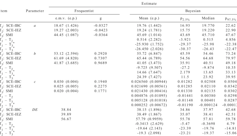
There were no marked differences among the estimates of the parameters obtained by the two methods for any of the variables studied. However, the Bayesian methodology allowed comparison of the estimates of the parameters for
the different treatments but these comparisons could not be made by the frequentist methodology, as already reported. The a parameter estimates (Table 2) for corn silage differed from the estimates of the other treatments (the zero value was not contained in the credibility interval). The same occurred for the b parameter estimates. The c
parameter estimates differed only between the elephant grass with enzyme bacterial inoculation and the corn silage. The effective degradability (DE) estimate for the corn silage (SMI) was significantly greater than those calculated for the elephant grass silages (SCE-IBC e SCE-IEZ).
The corn silage presented greater total degradability, while the elephant grass silages were similar.
The a parameter estimates differed among the silages (Table 3). The b parameter estimates differed between the corn silage and the elephant grass silages, while the c
parameter estimates differed only among the elephant grass silages. The effective degradability estimate of the elephant grass silage with bacterial inoculant was lower than those calculated for the other silages.
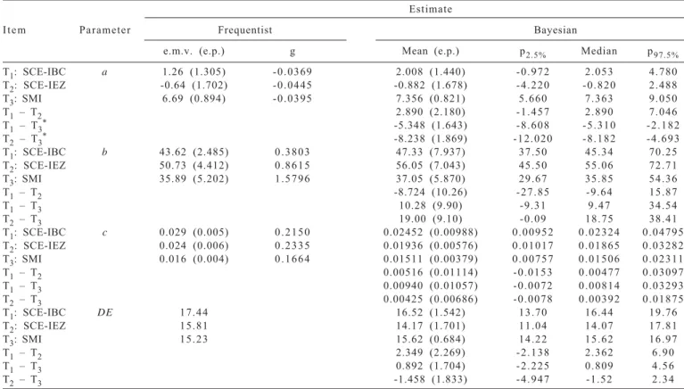
The corn silage differed from the others regarding the
a parameter estimates (Table 4). The b and c parameter estimates did not differ among the silages, even for the effective degradability.
T1: SCE-IBC a 18.67 (1.426) - 0 . 0 3 2 7 19.76 (1.442) 1 6 . 9 3 1 9 . 7 7 0 2 2 . 6 2 T2: SCE-IEZ 19.27 (2.003) - 0 . 0 4 2 3 19.24 (1.781) 1 5 . 7 5 1 9 . 2 2 0 2 2 . 9 0 T3: SMI 44.45 (1.087) - 0 . 0 3 6 4 45.69 (1.014) 4 3 . 6 9 4 5 . 7 1 0 4 7 . 6 7 T1 – T2 0.514 (2.282) - 3 . 9 2 1 0 . 5 1 5 4 . 8 5 6 T1 – T3* -25.930 (1.752) - 2 9 . 3 7 - 2 5 . 9 8 - 2 2 . 3 8
T2 – T3* -26.450 (2.026) - 3 0 . 3 7 - 2 6 . 4 3 - 2 2 . 4 7
T1: SCE-IBC b 53.12 (2.594) 0 . 2 9 2 0 55.72 (6.847) 4 5 . 5 9 5 4 . 4 6 7 3 . 2 4 T2: SCE-IEZ 61.69 (4.820) 0 . 7 3 0 7 65.44 (6.789) 5 4 . 5 6 6 4 . 6 8 7 9 . 9 7 T3: SMI 41.87 (3.685) 0 . 9 6 8 9 41.05 (3.473) 3 5 . 9 1 4 0 . 5 1 4 9 . 1 8
T1 – T2 -9.725 (9.507) -27.2 - 9 . 8 7 4 1 0 . 3 5
T1 – T3* 14.66 (7.647) 2 . 1 7 9 1 3 . 6 5 3 3 . 1 3
T2 – T3* 24.39 (7.427) 1 1 . 5 2 3 . 9 2 3 9 . 9 5
T1: SCE-IBC c 0.030 (0.004) 0 . 1 9 4 0 0.026560 (0.00944) 0 . 0 1 2 8 2 0 . 0 2 5 0 8 0 . 0 5 0 4 T2: SCE-IEZ 0.025 (0.005) 0 . 2 2 7 5 0.021690 (0.00561) 0 . 0 1 2 8 5 0 . 0 2 1 1 0 0 . 0 3 4 2 T3: SMI 0.020 (0.004) 0 . 1 7 7 1 0.021430 (0.00416) 0 . 0 1 3 3 0 0 . 0 2 1 3 5 0 . 0 3 0 2 T1 – T2 0.004876 (0.01095) -0.01441 0 . 0 0 3 8 0 0 . 0 2 9 8 T1 – T3 0.005128 (0.01018) -0.01148 0 . 0 0 4 0 1 0 . 0 2 8 7 T2 – T3* 0.000252 (0.00672) -0.01190 - 0 . 0 0 0 1 2 4 -0.00013
T1: SCE-IBC DE 3 8 . 8 4 38.15 (1.896) 3 4 . 8 6 3 7 . 9 7 4 2 . 6 8 T2: SCE-IEZ 3 9 . 8 9 38.49 (1.867) 3 5 . 0 7 3 8 . 4 1 4 2 . 5 1 T3: SMI 5 6 . 6 7 57.79 (0.9959) 5 5 . 7 8 5 7 . 8 1 5 9 . 7 8 T1 – T2 -0.3413 (2.629) - 5 . 4 7 - 0 . 3 6 9 8 4 . 7 9 T1 – T3* -19.64 (2.143) - 2 3 . 3 9 - 1 9 . 7 6 - 1 4 . 8 1
T2 – T3* -19.3 (2.098) - 2 3 . 2 1 - 1 9 . 3 7 - 1 5 . 0 6
* Significant difference at 5%. T1: SCE-IBC = elephant grass silage with bacterial inoculant; T2: SCE-IEZ elephant grass silage with enzyme bacterial inoculate and T3: SMI - corn silage; e.m.v. (e.p.) = maximum likelihood estimates (standard error); g = hougaard asymmetry coefficient; p2.5% and p97.5% = upper and lower limits, respectively, of the credibility interval.
Estimate
I t e m Parameter Frequentist Bayesian
e.m.v. (e.p.) g Mean (e.p.) p2.5% Median p97.5%
Estimate
I t e m Parameter Frequentist Bayesian
e.m.v. (e.p.) g Mean (e.p.) p2.5% Median p97.5%
T1: SCE-IBC a 26.73 (2.40) - 0 . 0 5 7 7 26.09 (2.591) 2 0 . 5 0 2 6 . 2 2 3 0 . 8 5 T2: SCE-IEZ 48.16 (1.58) - 0 . 0 5 4 1 48.58 (1.062) 4 6 . 3 3 4 8 . 6 1 5 0 . 6 9 T3: SMI 51.80 (1.23) - 0 . 0 5 2 4 51.84 (0.807) 5 0 . 1 6 5 1 . 8 6 5 3 . 5 1 T1 – T2* -22.49 (2.776) - 2 8 . 4 1 - 2 2 . 4 1 - 1 7 . 2 9 T1 – T3* -25.76 (2.705) - 3 1 . 5 4 - 2 5 . 6 4 - 2 0 . 7 9
T2 – T3* -3.26 (1.314) -5.94 -3.24 -0.68
T1: SCE-IBC b 45.46 (3.29) 0 . 0 7 6 2 43.90 (3.185) 3 8 . 0 2 4 3 . 7 0 5 0 . 7 7 T2: SCE-IEZ 37.44 (3.50) 0 . 8 0 0 3 41.33 (5.431) 3 4 . 0 7 4 0 . 0 5 5 4 . 8 4 T3: SMI 28.63 (2.21) 0 . 4 4 6 1 28.98 (1.675) 2 6 . 0 5 2 8 . 8 7 3 2 . 4 0
T1 – T2 2.58 (6.365) - 1 2 . 0 0 3 . 4 1 1 2 . 5 2
T1 – T3* 14.93 (3.600) 8 . 3 1 1 4 . 7 4 2 2 . 5 7 T2 – T3* 12.35 (5.716) 3 . 7 3 1 1 . 2 7 2 6 . 6 8 T1: SCE-IBC c 0.042 (0.009) 0 . 4 0 2 2 0.04590 (0.013140) 0 . 0 2 3 6 3 0 0 . 0 4 4 6 7 0 . 0 7 6 5 4 T2: SCE-IEZ 0.026 (0.007) 0 . 2 9 8 6 0.01893 (0.005685) 0 . 0 0 9 1 9 8 0 . 0 1 8 5 4 0 . 0 3 1 2 3 T3: SMI 0.031 (0.007) 0 . 3 1 2 6 0.02956 (0.005007) 0 . 0 1 9 0 7 0 0 . 0 2 9 7 0 0 . 0 3 9 0 5 T1 – T2* 0.02697 (0.014090) 0 . 0 0 2 8 2 2 0 . 0 2 5 6 3 0 . 0 5 8 2 9 T1 – T3 0.01634 (0.014000) - 0 . 0 0 7 3 2 7 0 . 0 1 4 9 4 0 . 0 4 7 9 9 T2 – T3 -0.01062 (0.00765) - 0 . 0 2 4 6 6 0 -0.01083 0 . 0 0 5 1 6 T1: SCE-IBC DE 4 7 . 6 0 46.71 (1.713) 4 3 . 4 5 4 6 . 6 5 5 0 . 3 2 T2: SCE-IEZ 6 1 . 1 3 59.46 (1.067) 5 7 . 4 3 5 9 . 4 4 6 1 . 6 3 T3: SMI 6 3 . 7 4 62.50 (1.055) 6 0 . 2 6 6 2 . 5 7 6 4 . 4 8 T1 – T2* -12.75 (2.007) - 1 6 . 6 7 - 1 2 . 8 2 -8.67 T1 – T3* -15.78 (2.024) - 1 9 . 6 3 - 1 5 . 8 8 - 1 1 . 5 1
T2 – T3 -3.03 (1.496) -5.91 -3.04 0 . 1 7
* Significant difference at 5%. T1: SCE-IBC = elephant grass silage with bacterial inoculant; T2: SCE-IEZ elephant grass silage with enzyme bacterial inoculate and T3: SMI - corn silage; e.m.v. (e.p.) = maximum likelihood estimates (standard error); g = Hougaard asymmetry coefficient; p2.5% and p97.5% = upper and lower limits, respectively, of the credibility interval.
Table 3 - Frequentist estimates and estimates of the parameters of the model and the crude protein effective degradability
* Significant difference at 5%. T1: SCE-IBC = elephant grass silage with bacterial inoculant; T2: SCE-IEZ elephant grass silage with enzyme bacterial inoculate and T3: SMI - corn silage; e.m.v. (e.p.) = maximum likelihood estimates (standard error); g = Hougaard asymmetry coefficient; p2.5% and p97.5% = upper and lower limits, respectively, of the credibility interval.
Estimate
I t e m Parameter Frequentist Bayesian
e.m.v. (e.p.) g Mean (e.p.) p2.5% Median p97.5%
T1: SCE-IBC a 1.26 (1.305) - 0 . 0 3 6 9 2.008 (1.440) - 0 . 9 7 2 2 . 0 5 3 4 . 7 8 0 T2: SCE-IEZ -0.64 (1.702) - 0 . 0 4 4 5 -0.882 (1.678) - 4 . 2 2 0 - 0 . 8 2 0 2 . 4 8 8 T3: SMI 6.69 (0.894) - 0 . 0 3 9 5 7.356 (0.821) 5 . 6 6 0 7 . 3 6 3 9 . 0 5 0 T1 – T2 2.890 (2.180) - 1 . 4 5 7 2 . 8 9 0 7 . 0 4 6 T1 – T3* -5.348 (1.643) - 8 . 6 0 8 - 5 . 3 1 0 - 2 . 1 8 2
T2 – T3* -8.238 (1.869) - 1 2 . 0 2 0 - 8 . 1 8 2 - 4 . 6 9 3
T1: SCE-IBC b 43.62 (2.485) 0 . 3 8 0 3 47.33 (7.937) 3 7 . 5 0 4 5 . 3 4 7 0 . 2 5 T2: SCE-IEZ 50.73 (4.412) 0 . 8 6 1 5 56.05 (7.043) 4 5 . 5 0 5 5 . 0 6 7 2 . 7 1 T3: SMI 35.89 (5.202) 1 . 5 7 9 6 37.05 (5.870) 2 9 . 6 7 3 5 . 8 5 5 4 . 3 6 T1 – T2 -8.724 (10.26) - 2 7 . 8 5 - 9 . 6 4 1 5 . 8 7
T1 – T3 10.28 (9.90) -9.31 9 . 4 7 3 4 . 5 4
T2 – T3 19.00 (9.10) - 0 . 0 9 1 8 . 7 5 3 8 . 4 1
T1: SCE-IBC c 0.029 (0.005) 0 . 2 1 5 0 0.02452 (0.00988) 0 . 0 0 9 5 2 0 . 0 2 3 2 4 0 . 0 4 7 9 5 T2: SCE-IEZ 0.024 (0.006) 0 . 2 3 3 5 0.01936 (0.00576) 0 . 0 1 0 1 7 0 . 0 1 8 6 5 0 . 0 3 2 8 2 T3: SMI 0.016 (0.004) 0 . 1 6 6 4 0.01511 (0.00379) 0 . 0 0 7 5 7 0 . 0 1 5 0 6 0 . 0 2 3 1 1 T1 – T2 0.00516 (0.01114) - 0 . 0 1 5 3 0 . 0 0 4 7 7 0 . 0 3 0 9 7 T1 – T3 0.00940 (0.01057) - 0 . 0 0 7 2 0 . 0 0 8 1 4 0 . 0 3 2 9 3 T2 – T3 0.00425 (0.00686) - 0 . 0 0 7 8 0 . 0 0 3 9 2 0 . 0 1 8 7 5 T1: SCE-IBC DE 1 7 . 4 4 16.52 (1.542) 1 3 . 7 0 1 6 . 4 4 1 9 . 7 6 T2: SCE-IEZ 1 5 . 8 1 14.17 (1.701) 1 1 . 0 4 1 4 . 0 7 1 7 . 8 1 T3: SMI 1 5 . 2 3 15.62 (0.684) 1 4 . 2 2 1 5 . 6 2 1 6 . 9 7 T1 – T2 2.349 (2.269) - 2 . 1 3 8 2 . 3 6 2 6 . 9 0 T1 – T3 0.892 (1.704) - 2 . 2 2 5 0 . 8 0 9 4 . 5 6
T2 – T3 -1.458 (1.833) - 4 . 9 4 7 -1.52 2 . 3 4
Conclusions
The Bayesian methodology can be applied without restriction to data of this nature. For the data in the present study, the estimates did not differ for the non-linear curve parameters for either method. However, when using the Bayesian methodology it is possible to proceed to the comparisons among these parameters, considering the different factors of an experiment coherently, bearing in mind their a posteriori distribution, without having to resort, for example, to asymptotic procedures and incoherent results through frequentist theories.
References
AGRICULTURAL RESEARCH COUNCIL – ARC. The nutrient requirements of ruminant livestock. Slough: Commonwealth Agricultural Bureaux, 1984. 45p.
BATES, D.M.; WATTS, D.L. Relative curvature measures of nonlinearity (with discussions). Journal the Royal Statistical Association B, v.22, p.41-88, 1988.
BEST, N.G.; COWLES, M.K.; VINES, S.K. CODA: Convergence d i a g n o s t i c s a n d o u t p u t a n a l y s i s s o f t w a r e f o r G i b b s sampler output. Version 0.3. Cambridge: MRC Biostatistics Unit, 1995. (CD-ROM).
CARVALHO, G.G.P; GARCIA, R.; PIRES, A.J.V. et al. Degradação ruminal de silagem de capim-elefante emurchecido ou com diferentes níveis de farelo de cacau. Revista Brasileira de Zootecnia, v.37, n.8, p.1347-1354, 2008.
GEWEKE, J. Evaluating the accuracy of sampling-based approaches to the calculation of posterior moments (with discussion). In: BERNARDO, J.M. et al. (Eds.). Bayesian statistics 4. Oxford: Oxford University Press, 1992. p.169-193.
HEIDELBERGER, P.; WELCH, P. Simulation run length control in the presence of an initial transient. Operations Research,
v.31, p.1109-1144, 1983.
KATSUKI, P.A.; MIZUBUTI, I.Y.; PEREIRA, E.S. et al. Cinética ruminal da degradação de nutrientes da silagem de milho em ambiente ruminal inoculado com diferentes aditivos1. Revista Brasileira de Zootecnia, v.35, n.6, p.2421-2426, 2006. M A RT I N S , A . S . ; V I E I R A , P. F. ; B E R C H I E L L I , T. T . e t a l .
D e g r a d a b i l i d a d e i n s i t u e o b s e r v a ç õ e s m i c r o s c ó p i c a s d e volumosos em bovinos suplementados com enzimas fibrolíticas e x ó g e n a s . Revista Brasileira de Zootecnia, v. 3 6 , n . 6 , p.1927-1936, 2007.
MEHREZ, A.Z.; ORSKOV, E.R. A study of the artificial fiber bag technique for determining the digestibility feeds in the rumen.
Journal of agricultural Science, v.88, n.3, p.645-650, 1977. O R S K O V, E . R . ; M c D O N A L D , I . T h e e s t i m a t i o n o f p r o t e i n degradability in the rumen from incubation measurements weighted according to rate of passage. Journal of Agricultural Science, v.92, n.1, p.499-503, 1979.
PAULINO, C.D. et al. Estatística Bayesiana. Lisboa: Fundação Calouste Gulbenkian, 2003. 446p.
P R A D O , I . N . ; M O R E I R A , F. B . ; Z E O U L A , L . M . e t a l . Degradabilidade in situ da matéria seca, proteína bruta e fibra e m d e t e r g e n t e n e u t r o d e a l g u m a s g r a m í n e a s s o b p a s t e j o c o n t í n u o . R e v i s t a B r a s i l e i r a d e Z o o t e c n i a, v. 3 3 , n . 5 , p.1332-1339, 2004.
S TAT I S T I C A L A N A LY S I S S Y S T E M - S A S . SAS (Statistics analysis system). Version 8.02. Cary: SAS Institute, 2003. (CD-ROM).
SILVA, D.J.; QUEIROZ, A.C. Análise de alimentos: métodos químicos e biológicos. Viçosa, MG: Universidade Federal de Viçosa, 2002. 235p.
RATKOWSKY, D. Nonlinear regression modeling. New York and Basel: Marcel Dekker, 1983. 276p.
RATKOWSKY, D. Handbook of nonlinear regression models. Marcel Dekker: New York and Basel, 1990. 241p.
SPIEGELHALTER, D.J.; THOMAS, A.; BEST, N.; GILKS, W.
BUGS - Bayesian inference using gibbs sampling. Cambridge. Version 1.4.2 Cambridge: MRC Bioestatistics Unit, 1994. v.1. (CD-ROM).