Fractal Rain Distributions and Chaotic Advection
Ronald Dickman
Departamento de F´ısica, ICEx, Universidade Federal de Minas Gerais,
Caixa Postal 702, 30161-970 Belo Horizonte, Minas Gerais, Brazil
Received on 1st December, 2003
Localized rain events have been found to follow power-law distributions over several decades, suggesting par-allels between precipitation and seismic activity [O. Peters et al., PRL88, 018701 (2002)]. Similar power laws can be generated by treating raindrops as passive tracers advected by the velocity field of a two-dimensional system of point vortices [R. Dickman, PRL90, 108701 (2003)]. Here I review observational and theoretical aspects of fractal rain distributions and chaotic advection, and present new results on tracer distributions in the vortex model.
1
Introduction
Complex systems often exhibit fractal or power-law scaling; Earth’s atmosphere is no exception. Fractal rain distribu-tions have been known for at least two decades [1, 2, 3], while recent analyses indicate that durations of dry intervals, and the size of rain events, follow power laws [4, 5]. The similarity between the latter observations and scaling laws in seismic activity suggests a parallel between rain and earth-quakes, and a possible connection with the phenomenon of self-organized criticality [5, 6].
Atmospheric motion is turbulent, particularly in the vicinity of storms, and various aspects of turbulent flow fol-low power laws over many orders of magnitude [7, 8, 9]. Even in the absence of fully developed turbulence, un-steady flow may stretch and fold an initially compact region, leading to a highly convoluted, nonuniform density of sus-pended particles or droplets [10, 11, 12] via chaotic advec-tion [13, 14]. In light of these observaadvec-tions, it is interesting to develop a model in which rain is anideal passive tracer
[15, 16]. In [17] it was shown that such a model is capable of producing power-law-distributed event sizes and durations.
In this paper I review some of the evidence for fractal rain distributions, and present new results on the spatial dis-tribution of tracers in the vortex model. Progress in fluid me-chanics depends heavily on numerical solution of the equa-tions of motion, which in turn represents one of the most challenging areas in computational physics, the theme of the present number.
In Sec. II, I survey observations of fractal rain distri-butions. Sec. III contains a brief discussion of SOC-like approaches, while Sec. IV reviews results on tracer-particle dynamics in a fluid undergoing chaotic advection. I define the vortex model in Sec. V, which also includes a summary of previous findings and some recent extensions. Sec. VI presents new results on spatial distributions of tracers in the vortex model. The paper closes in Sec. VII with a summary and discussion of open questions.
2
Fractal rain distributions
Discussions of fractal rain distributions go back at least to the work of Lovejoy and Mandelbrot [1] who presented a model with a single fractal dimension. The distribution in question involves a time series of durationTand a fixed ob-servation point orstation. The observation interval is parti-tioned intoN =T /τsubintervals of durationτ, each char-acterized as rainy (a nonzero amount of rain is detected at the station in this interval) or dry. The functionr(τ)is then defined as the number of rainy subintervals at scaleτ. Ols-son et al. found that this distribution follows a power law, r ∼ τ−γ, withγ ≃ 0.8, over a certain range of durations
[2]. Note that forτ ≈ T, r → N (all subintervals are rainy), while forτmuch shorter than the characteristic time between raindrops,rsaturates at a valueMequal to the total number of raindrops incident on the station during the inter-valT. Between these simple limits,r(τ)may exhibit non-trivial behavior reflecting correlations in the generation or dynamics of raindrops. Now, if the arrival times of the rain-drops were mutually independent (so that the time interval between successive drops at the detector were exponentially distributed), the number of dropsn(τ)in a given subinterval would be Poisson-distributed with meann(τ)=mτ, with m=M/T, and we would haver(τ) = (T /τ)(1−e−mτ).
Thus a power law distribution withγ <1rules out a sim-ple “independent event” model, suggesting some nonlinear mechanism behind the observed rainfall statistics.
The observations of Olsson et al. (from Sweden) were later corroborated by Lavergnat and Gol´e [3] in an experi-ment performed near Paris. The latter study generated data on raindrop arrival times and sizes over a 14-month period, and confirmed the scaling r ∼ τ−0.82
over six orders of magnitude (from 0.01 to 104
minutes). Other important conclusions from this study are: (1) the raindropdiameter
mm; (2) the distribution of time intervals between raindrops can be fit to a so-called bi-Pareto distribution over about nine orders of magnitude. This distribution involves two power law regimes, one for short times (drops associated with a given storm) another for long times (intervals between suc-cessive storms). On the basis of their analysis Lavergnat and Gol´e conclude that the waiting timeDbetween successive rain events is power-law distributed: Pd(D)∼ D−τD with
τD = 1.68. (ForD ≈one day the probability densityPd
decays rapidly; droughts longer than a week or so were not seen in their experiment.)
Convincing evidence for a multifractalspatial distribu-tion of raindrops in storms, on scale from 1 cm up to meters, was very recently reported by Lovejoy et al. [18]. An impor-tant conclusion of these authors is that there is no meaning-ful way to describe rain content in the atmosphere in terms of a smoothly varying density, since large fluctuations are present at all scales. The authors suggest turbulence as the reason for the fluctuations in raindrop distribution.
Recently a large time-series (six months) from radar ob-servations on the Baltic coast became available under the BALTEX project [19]. The radar station determines the quantity of rain falling in a 1 m2
column of the atmosphere. Arrival times of individual raindrops are not resolved, but the total amount of rain above the station at each 1 min. interval is registered. The threshold for detection is 0.005 mm/h; intervals with a precipitation rate above this thresh-old have a nonzero rateq(t), otherwise q(t) = 0for that interval. In their analysis of the BALTEX data, Peters et al. focus on rain events, defined as sequences of consecutive intervals with nonzero rainfall [4, 5]. A series of consec-utive intervals having zero rain defines a drought. The in-tensityI=tq(t)of a rain event is the rainfall integrated over its duration. Peters, Hertlein and Christensen found that the distribution of rain-event sizes at the Baltic coast station follows a power law over at least three decades. Drought durations are also power-law distributed over the range of several minutes to about a week, with a significant perturba-tion apparently reflecting diurnal variaperturba-tion. The power laws identified by Peters et al. may be expressed in the form
Pi(I)∼I−τI (1)
and
Pd(D)∼D−τD , (2)
wherePi and Pd are the probability distributions for rain
event intensities, and for drought durations, and the expo-nents are found to take the values
τI = 1.36 τD= 1.42 (3)
These authors emphasize the similarities between these dis-tributions and those found for earthquakes, suggesting a par-allel with self-organized criticality to be discussed in the fol-lowing section.
Taken as a whole, the observations of Olsson et al., Lavergnat and Gol´e, Lovejoy and co-workers, and Peters et al. present a very strong case for fractal or multifractal distributions of rain at a given position over time, and in
space, at a given instant [20]. The universalityof the ob-served distributions is less clear. First, the time series all come from the north of Western Europe, where prolonged dry periods are evidently rare. The central region of Minas Gerais, Brazil (to cite one example) experiences a dry spell of several months each year, and might therefore exhibit a different distribution of droughts. The Paris and Sweden experiments yielded similar values (γ= 0.82) for the expo-nent characterizing the fractal distribution in time, while the BALTEX data yieldγ ≃ 0.55[5]. On the other hand, the Paris results suggestτD= 1.68, considerably larger than the
Baltic observations. Observations from other sites (in partic-ular, from other regions of the world, including continental sites, and oceans), are needed to confirm the generality of power laws, and the range of exponent values.
3
Rain and Self-organized criticality
Peters, Hertlein and Christensen noted a striking similar-ity between the scaling laws they found in the rain data and those known for earthquakes. Specifically, earthquake magnitudesM (defined in terms of energy released) follow the Gutenberg-Richter lawPm(M) ∼ M−τM [21], while
the waiting time between earthquakes in a given region fol-lows a power-law known as Omori’s law [22, 23]. This suggests a parallel between precipitation in the atmosphere and relaxation of the Earth’s crust at stressed tectonic-plate boundaries [5]. In the context of seismology, cooperative relaxation due to elastic interactions and nonlinear friction is captured by block-spring models [24, 25] or, in much-reduced fashion, by sandpile models [6]. The latter have attracted much attention as the principal example of the self-organized criticality paradigm for scale-invariance in natu-ral, far-from-equilibrium systems [6, 26, 27].
Indeed, sandpile-like models of rainfall have been stud-ied [28, 29]. They involve the directed motion of raindrops such that when a given cell contains more than a certain number of drops, the latter move to cells at the level be-low. That such a model yields power-law distributions for sizes of certain kinds of events is not surprising, as this is an intrinsic feature of sandpile models [26, 30]. (It is less clear how to define thedurationof a rain event, since sandpiles represent a singular limit in which event durations cannot be measured on the same time scale as intervals between events [31, 32].)
But if certain aspects of rain distributions resemble those of avalanches in sandpile-like models, the underlying physics remains obscure. While it may yet prove possible to explain the observed power laws in terms of an open, driven dissipative system [28, 29, 33], there is no obvious reason for the formation or precipitation of one raindrop to provoke similar events nearby. Given the attendant release of latent heat, one might instead expect a self-limiting tendency in condensation.
While it is hard to see how direct interactions between rain-drops over a mean interparticle distance of 10 cm [18] could lead to clustering, the drops are of course highly influenced by the motion of the surrounding air. The latter is gener-ically turbulent [9], and as such is characterized by scale-invariant velocity and energy distributions. Thus it appears more promising to seek the explanation for power-law dis-tributions in atmospheric fluid dynamics.
4
Chaotic Advection
In this and the following sections we will be interested in the dynamics of passive tracer particles in a fluid. Such a particle follows the local velocity of the fluid at each mo-ment, so that its trajectory is that of a fluid particle. The fluid velocity is not affected by the tracers. As such, a tracer rep-resents an idealized limiting case of a very small, neutrally buoyant particle immersed in the fluid. (Tracers are small in the sense that (1) their inertia is negligible and (2) the fluid velocity varies little over the diameter of the tracer.) The idea of the model to be developed below is that raindrops can be treated, to a first approximation, as passive tracers, even though they are much denser than air, and not always “small.” This study should nevertheless provide a prelimi-nary indication of how atmospheric motion can affect the distribution of the raindrops.
Now, if the fluid motion is turbulent, the distribution of passive tracer particles should also exhibit scale-invariant properties [12, 15, 16]. An important example is Richard-son’s law, the empirical result that in turbulent flow, the mean-square separationℓtbetween a pair of tracers at time
t, given an initial separation ofℓ0, grows∼ ℓ 4/3
0 . If two
or more tracers are released at nearby points, we can study how their trajectories separate over time, leading to the no-tion of chaotic tracer mono-tion: trajectories that separate ex-ponentially rapidly with time. A flow need not be turbulent to exhibit chaos in this sense. Relatively simple flows, such as the van Karman vortex street or flows generated by sys-tems of point vortices exhibit this property. Aref showed that this phenomenon, known as chaotic advectionor La-grangian chaos, appears in systems of as few as four mutu-ally interacting vortices [13, 14]. (The vortex system, which is central to the model developed here, will be described in detail below.)
Some aspects of chaotic advection can be understood in a general way using elementary notions from dynamical sys-tems theory. Consider an incompressible fluid restricted to a finite volume. A stagnation point in such a flow is a hy-perbolic fixed point: due to volume conservation, the fluid is attracted to this point along one direction, and repelled along another. As a result, a fluid element that passes near the hy-perbolic point is stretched along one direction, compressed along the other. As stretching continues, the element must double back on itself since it is confined to a finite region. Repeated encounters with hyperbolic points lead to iterated distortions of the kind described above. Thus a fluid element undergoes repeated stretching and folding similar to the dis-tortions leading to chaos in simple model systems such as
the baker’s transformation [35].
Flow fields with chaotic advection may also exhibit un-stable periodic orbits with fractal structure[11]; tracers (as well as particles with non-negligible inertia) may spend long periods of time in the vicinity of these orbits [36]. The ef-fect, once again, is that an initially compact region becomes highly extended along one direction, and contracted in the other, and repeatedly folded, yielding a self-similar struc-ture of bands reminiscent of a strange attractor in a chaotic dynamical system.
Summarizing, the motion of tracer particles in even moderately complex flows can yield chaotic trajectories and scale-invariant spatial distributions. This suggests treating rain as a collection of passive tracers moving in a chaotic or turbulent velocity field. The raindrops are released in a localized condensation event, and then advected by the air before being detected at or above a given point on Earth’s surface.
What would a reasonably complete model of this process look like? Even ignoring thermodynamic aspects (evap-oration and re-condensation of rain, with attendant latent-heat and buoyancy effects), we would need to treat a three-dimensional atmosphere whose density falls off exponen-tially with height, and integrate the Navier-Stokes equation for an incompressible fluid subject to suitable boundary and initial conditions, (including a driving term at large scales to compensate small-scale dissipation, if we wish to study a stationary state), at a Reynolds number characteristic of turbulent motion [37]. To include the possibility of convec-tion we would need to implement (at least) the Boussinesq approximation, allowing the density to vary linearly with temperature, and including heat transfer in the description [38, 39]. Such a study poses a great challenge to presently avaliable computational tools. In particular, faithful repre-sentation of fully developed turbulence appears (due to the number of degrees of freedom involved) computationally nonviable, so that reduced descriptions such as large-eddy simulation or a shell model are required [7, 8].
While semi-realistic simulation seems a worthy objec-tive for future study, in this work I consider a radically sim-plified model, which can serve as a proof of principle of the idea that fractal rain distributions derive from chaotic advec-tion. The model eliminates nearly all atmospheric processes and takes advantage of a physical system (point vortices) affording a vast reduction in computational complexity, as explained in the next section.
5
Computational Model
irro-tational, i.e.,∇ ×u= 0. Potential flow solutions of Euler’s equation satisfy the principle of linear superposition.
The velocity field is built up out of complex potentials of the form
φ=−iK
2πln(x+iy) (4) corresponding to the velocity field (in polar coordinates)
uθ= K
2πr , ur= 0. (5) (The circulationK is the line integral of the velocity over any circuit including the origin;∇×u= 0except at the ori-gin, where the velocity is evidently singular.) We construct more complicated flows by superposing vortices at different pointsrj. (The vortex is an extended object;rjdenotes the position of the singularity.) In a system ofNV point
vor-tices, each vortexj moves in the velocity field defined by the superposition of all vortices except vortexj itself [41]. (ForNV ≤ 3 the system is integrable [14].) Thus, in this
rather special case we can construct a complex fluid motion
without solving the Euler equation, by integrating the mo-tion of a system ofNpoint particles. This makes the vortex system particularly attractive for simulating incompressible, inviscid flow.
Point-vortex systems have been used for some time in studies of two-dimensional turbulence [7, 43, 44] and of chaotic advection [13, 14], and appear to be relevant to at-mospheric dynamics on various scales [45]. Two interesting scaling properties of tracers in systems of four or more point vortices are worth noting [14]: (1) the tracers exhibit anoma-lous difusion, with the mean-square displacement growing ∼ t1.8
; (2) the lifetimes of vortex pairs follows a power-law distribution,P(s) ∼ s−2.7
. (Tracers are typically ex-cluded from the immediate vicinity of a vortex, but may on the other hand become trapped at the periphery of a vor-tex pair.) Compared with direct integration of the Euler or Navier-Stokes equations, the computational demands are or-ders of magnitude smaller. Of course, one is restricted to a two-dimensional, inviscid fluid. (In the three-dimensional case the vortices become vortex lines, which stretch and fold under the flow. But such a system may still offer computa-tional advantages.)
In Ref. [17] I study a system of interacting point vortices on the unit square with periodic boundaries. The velocity of vortexiis given by
vi =
j=i
Kj
2πr2
ij
ˆ
k×rij, (6)
whereKjrepresents the circulation of vortexj(equal
num-bers of clockwise and anticlockwise vortices are used), and
rij=ri−rj, under periodic boundaries, using the
nearest-image criterion. The velocityu(x,t) at an arbitrary pointx
in the plane (not occupied by a vortex) is given by a similar sum including contributions from all vortices. The number of vorticesNV ranges from 10 to 126.
Several types of vortex-strength distributions are stud-ied; the simplest assigns all vortices the same strength|K|. Other studies employ a hierarchical vortex distribution, de-fined as follows. The zeroth “generation” consists of a pair
of vortices withK = ±K0. Subsequent generations,n =
1, ..., ghave2n+1
vortices, with circulation|K|=K0/αn.
I studyα= 2, 3, and 4, usingg+1 = 5or 6 generations. The purpose of the hierarchical distribution is to provide struc-ture on a variety of length scales, without trying to repro-duce any specific energy spectrumE(k). The vortices are assigned random initial positions, but their subsequent evo-lution is deterministic [46].
Being point objects, the vortices possess no intrinsic length scale. (Note however that in the presence of other vortices, the ‘sphere of influence’ of vortexiis proportional toKi.) A characteristic length scale is the mean separation
∼ 1/√NV between vortices. The vortex system defines a
mean speedu=|u(x, t)| ∝K0√NV; an important time scale is τC ∼ 1/u, the typical time for a fluid particle to
traverse the system. A typical velocity field in a system of ten vortices (all of equal intensity) is shown in Fig. 1.
Figure 1. Velocity field in a system of ten vortices of equal strength.
A large number of tracers,Np = 10 000, are thrown at
random into a small region (a square of side 0.05), repre-senting a localized condensation event. (Alternatively, the tracer-laden region may be interpretated as a parcel of atmo-sphere of high humidity, destined to generate precipitation.) In the analysis of rain and drought events, the observation intervalT plays an important role. At time zero the vortices begin their motion, and the tracers are inserted. The dynam-ics is followed up to timeT, when the simulation ends.
In the model, ‘rain’ corresponds to the presence of one or more tracers in a very small predefined region or ‘weather station’, of linear dimension 0.01. At each step of the inte-gration, the number of particles ni(t)at each station i is
monitored. A sequence of nonzero occupation numbers at a given station constitutes a rain event, just as in the radar ob-servations [4]; the intensity of a rain event isI=tni(t)
whichni(t)>0. In caseni = 0, stationiis said to
experi-ence a drought. The durations of droughts and of rain events are likewise monitored over a time intervalT.
Figure 2. Positions of 104
tracers (small points) and 10 vortices (open circles, clockwise circulation, filled, anticlockwise), at times 0.46 (a), 0.48 (b) and 0.50 (c).
Fig. 2 shows successive configurations of a system of 104
particles and 10 vortices of equal intensity, at times 0.46, 0.48 and 0.50, under conditions such that |u(x, t)| = 4.
(ThusT = 0.5 corresponds to 2τC.) In this example the
tracer-bearing region has become wrapped around a vor-tex pair, and becomes increasingly stretched. The tracers are widely scattered, but their distribution remains highly nonuniform, characterized by bands of high particle con-centration. (The tracer-free regions centered on the vortex pair arise because the fluid trajectories circulate about the vortices, so that tracers cannot penetrate this region from outside.) At later times (see Fig. 3, forT = 8τC) tracers are
more uniformly distributed, but there are again empty re-gions centered on vortices or vortex pairs. (In these studies the tracers were released from a region of size0.01×0.01 to provide enhanced spatial resolution.)
Figure 3. Positions of5×104
tracers at time8τC, for the same conditions as Fig. 2.
Varying the vortex distribution and observation interval T, the following trends emerge. ForT /τCin the range 0.1
- 2, power-law rain-intensity and drought duration distribu-tions are found, as in Eqs. (1) and (2). The rain-intensity dis-tribution follows a power law over 4 - 5 1/2 decades, with an exponentτI in the range 0.93 - 1.02. The drought-duration
distribution decays with a somewhat larger exponent, 1.12 -1.16, and follows a power law over 3 - 4 decades. Larger ex-ponent values are associated with higher values ofα; these yield somewhat smaller ranges for the power laws. Con-versely, the largest power-law range, and smallest exponent values, are observed when all vortices are of equal strength. There is no significant difference between the distributions obtained initially and those found after the vortices have had some time to evolve, suggesting that the equilibration pro-cess expected in two-dimensional turbulence [43, 44] is not important as regards rain and drought statistics.
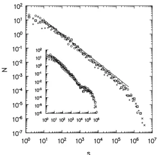
Systems with varying numbers of vortices yield similar distributions, if we scale the intensityK ∼1/√NV. This
is seen from the data collapse in Fig. 4, in which results for systems of 10, 20, 50 and 100 vortices (withNp = 104,
T ≃ 0.85τc, and K = 0.3 forNV = 10), are shown.
turbulence.
Figure 4. Rain-size (main graph) and drought-duration (inset) dis-tributions in systems of vortices of equal strength,T ≃0.85τc.◦:
NV = 10;×:NV = 20;✷:NV = 50;+:NV = 100. The vor-tex intensityKis scaled∼1/√NV in these studies. The straight lines have slopes of -1.01 (rain size) and -1.13 (drought).
For larger values ofT /τC the particles are more
dis-persed, and the rain size and drought duration follow a stretched-exponential formPi(I) ∝ exp(−CIβ)withC a
constant andβ ≃ 0.5. Even for large values ofT /τC (up
to 200 in the present study), the distributions decay more slowly than an exponential, showing that the tracer density is non-Poissonian.
The results of [17] may be summarized as showing scale-invariant rain-size and drought-duration distributions for intervals such that the tracers remain highly clustered. Although the decay exponents are somewhat smaller than those obtained from observational data (1.36 and 1.42 for rain size and drought duration, resp. [4]), the simulations also show the drought duration decaying more rapidly than that for rain event sizes. For conditions under which the rain is more thoroughly dispersed, simulations yield stretched-exponential distributions. It is worth noting that the finding of non-power-law distributions at longer times does not sig-nal an inability of the model to reproduce the observatiosig-nal results. Rain, after all, does not remain in the air indefi-nitely. (It would, of course, be interesting to have some way of comparing the model timescaleτC with the typical
res-idence time of rain in the atmosphere.) The tendency to-ward a more uniform tracer distribution at times≫ τC is
in fact exagerated by the periodic boundaries of the model, and might occur more slowly under a corresponding vortex dynamics in the atmosphere.
Even in a system as simple as that considered here, there is a large parameter space to be explored: number, circula-tion, and intensity of vortices, size and shape of the initial particle-bearing region, observation timeT. To close this section I report some preliminary results on situations not considered in [17]. In all cases there are ten vortices, all of intensity 0.3, yielding|u(x, t)| = 4. A study in which
the tracers are released from a circular, rather than a square region yields the same exponentsτI andτD as found
pre-viously. Thus the shape of the initial region appears not to influence the event statistics.
It is natural to ask how relaxing the “neutrality condi-tion” (equal numbers of vortices with clockwise and anti-clockwise circulation) affects the event distributions, since there is no obvious reason to assume such neutrality. A study using all vortices with the same circulation again yields power-law distributions, but with somewhat different expo-nent values, depending on the observation time. Specifi-cally, forT = 0.8τCI findτI = 1.01(1)andτD= 1.10(2),
similar to the results for the neutral system, while forT = 1.2τC,τI = 1.21(1)andτD = 1.06(1). Thus, allowing a
net circulation results in a larger rain intensity exponent at longer times, while the drought exponent is slightly smaller. There is also evidence that releasing the tracers from a smaller region (of linear size 0.01 instead of 0.05) yields a largerτI and smallerτD. A study usingT = 0.5(and equal
numbers of clockwise and anticlockwise vortices), yielded τI = 1.10(2), whileτD ≃ 1.02. Although it is difficult to
draw firm conclusions from these preliminary results, they demonstrate the generality of power-law distributions at in-termediate times, while suggesting that exponent values may change depending on the flow regime.
6
Spatial Distribution of Tracers
As discussed in the preceding section, a very simple model of passive tracers in a velocity field defined by a system of point vortices is capable of yielding power-law rain-intensity and drought-duration distributions [17]. These re-sults for events at a fixed observation site suggest that the spatial arrangement of the tracers is somehow related to the event distributions. One might even hope to understand the scale-invariant event distributions as arising from a fractal tracer pattern as it sweeps over the observation site. In this section I present results on the spatial distribution of the tracer particles, which can be thought of as analogous to the distribution of rain over a region experiencing storms. The results are for systems with equal numbers of clockwise and anticlockwise vortices, all of equal intensityK.
As a first step, I consider the occupancy histogramN(n) upon partitioning the system into a fine mesh;N(n)denotes the number of elements with tracer occupancyn. The sim-ulation cell is divided into 104
square regions or boxes of side 0.01, and the box-occupancy histogram determined af-ter allowing the particle configuration evolve for a timeT. Recall that initially, a small number of boxes (25 or so) will have high occupancies, while the rest are empty. If the parti-cles tend toward a uniform distribution, we should expect the histogram to approach a Poisson distribution, with parame-ter 1 (there are 104
near occupancyn = 400is evident, a remnant of the ini-tially compact distribution. The histogram follows a power law N(n) ∼ n−ǫ, forn ≤ 200or so, with ǫ = 0.54(1)
forT = 0.2τC. AsT increases, the exponentǫbecomes
larger, and the histogram (on log scales) begins to curve downward, signaling a faster than power-law decay. For T = 0.5the histogram is well described by a stretched ex-ponential,N(n)∝exp[−const.×xβ]withβ ≃1/7. Thus
the histogram remains non-Poissonian even for rather long times. For a system of 100 vortices (withKscaled to main-tain the mean velocity constant as discussed in Sec. V), the histogram is power law (withǫ= 0.67) forT = 0.2τC, and
tends to a stretched exponential (withβ ≃1/5) for longer times.
Figure 5. Instantaneous occupancy histogramN(n)for boxes of side 0.01 in a system with 10 vortices, |K| = 0.3. Observation times:T = 0.2τc(filled squares);T = 0.4τc(✷);T = 0.8τc(•);
◦:T = 2τc(◦).
In principle, the fractal dimension of the instantaneous particle distribution may be determined in a manner analo-gous to the fractal time distribution described in Sec. III. That is, we divide the system into ever-finer partitions (for example, squares of side ℓ = 2−n forn = 1,2,3, ...) and
determine the number r(ℓ)of occupied squares at scaleℓ. For uncorrelated positions we expectr(ℓ)∝ℓ−2
away from the limits of very large or very small boxes. Applying this analysis to tracer configurations in the vortex system yields r(ℓ) ∝ ℓ−γ with γ = 1.8 - 1.9, depending on the
ob-servation time T and number of vortices. This may sig-nal an incipient fractal distribution, but a glance at a typi-cal configuration (Fig. 2) shows that at the times of inter-est, the particle-filled region is not a fully developed fractal structure, but rather is essentially linear, becoming increas-ingly stretched (and wound about one or more vortices), and folded as times goes on.
The observation of a stretched, linear tracer-bearing re-gion suggests that we distinguish two directions, locally par-allel and perpendicular to the elongated region. Observe
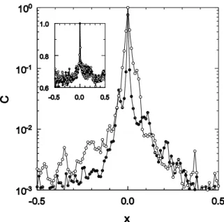
that the particle velocity is approximately parallel to the elongated direction. Thus it is of interest to define coordi-natesηandξat any instant, representing the distance from a given particleiin directions parallel and perpendicular to (respectively) its velocityvi. We study the tracer density as a function of distance from a randomly chosen particle, along these directions, effectively defining two-point corre-lation functionsC||(x)andC⊥(x). Fig. 6 shows that at time2τCthese functions are strongly peaked near the origin,
demonstrating a high degree of clustering, and thatC||(x) is generally greater thanC⊥(x), corresponding to the elon-gated linear regions typical of the particle configuration at intermediate times. The correlation functions at time8τC
(shown in the inset of Fig. 6) are much more uniform, away from the central peak, and appear to be isotropic.
Figure 6. Correlation functions (unnormalized) C||(x) (◦) and
C⊥(x)(•) on semi-log scales, in a system with ten vortices, ob-servation timeT = 2τC. Inset: a similar plot on linear scales for
T= 8τC.
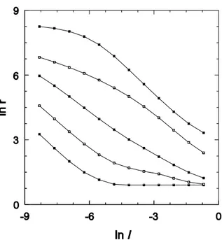
The configurations depicted in Fig. 2 suggest that the re-peated bands of particles (due to folding and/or wrapping around a vortex) possess a nested structure. We look for ev-idence of fractal structure along the perpendicular direction ξby dividing this axis (along a narrow swath,|η| ≤0.005) into segments of lengthℓ= 2−n, and determining the
num-ber of occupied segmentsr(ℓ)at scaleℓ. This function is shown for various observation times in Fig. 7. At the short-est timesr(ℓ)is constant for largerℓ, indicating that only a single box is occupied at the larger scales, due to the small insertion region (of length 0.01 here). At intermediate times there is evidence of fractal scaling (for example, atT = 2τC,
r∼ℓ−0.72
forℓ≤0.05). The slopeγ(away from the satu-ration region at smallℓ) appears to approach unity at larger times, again signaling a more uniform tracer distribution. (ForT = 2τCthe distributionr(ℓ)in theparalleldirection
Figure 7. Distributionr(ℓ)along a line perpendicular to the lo-cal velocity in a system of 10 vortices. Observation times (bottom to top)T /τC = 0.8, 1.2, 2.0, 4.0, and 8.0. (The data have been shifted vertically for visibility.)
Figure 8. Distributionr(ℓ)as in Fig. 7, but in a single realization with105
tracers released from a region of size 0.005. Observation times (bottom to top)T /τC = 2.4, 3.2, 4.0, 4.8, 5.6, 6.4 and 8.0. (The data have been shifted vertically for visibility.) The slopes of the straight lines are -1 and -0.47.
The results forr(ℓ)cited above represent averages over 5 - 10 configurations. High-resolution studies of single con-figurations (involving 105
tracers released from a region of linear size 0.005), yield power-law distributions in some cases, and stretched exponentials in others, for the same pa-rameter values. For example, in a system with ten vortices (|K|= 1.2,T = 4τC), one realization yielded a
stretched-exponential distribution withβ ≃ 0.1, while in other cases power laws (with γ = 0.45−0.55, over three or more
decades), were found. The stretched-exponential appears to be associated with an overall scattering of tracers (as in Fig. 3) while in the power-law case multi-band configura-tions predominate. Similar results are found in a system of 20 vortices. Fig. 8 shows how the distribution evolves over time in a typical high-resolution study. At short times, r(ℓ) ∼ 1/ℓfor small ℓ, indicating uncorrelated positions, while at intermediate times and length scales there is evi-dence of power-law scaling with γ ≈ 0.5, and at longer times the distribution can be fit to a stretched exponential withβ≃0.3.
Summarizing the results described in this section, there is preliminary evidence for a fractal tracer distribution at in-termediate times (on the order ofτC) associated with the
nested filamentary structures generated by stretching and folding of the particle-bearing region. The timescale for ob-servation of a fractal tracer density corresponds roughly to that associated with fractal rain and drought distributions. (One should recall, however, that the latter are accumulated from the time the tracers are released until timeT, whereas the tracer distributions discussed here are instantaneous.) It is easy to see that a fractal tracer distribution, swept past a fixed observation point, will generate power-law rain and drought distributions. It remains to make this connection more precise, a task complicated by the fact that the charac-teristics of the tracer distribution vary significantly over the observation period, and may also vary in space, as a glance at Fig. 2 suggests. This raises the possibility that the power-law distributions found in simulations and in actual mea-surements represent a superposition of distributions associ-ated with different kinds of regions or events. It would there-fore be of interest to identify simpler advection processes whose fractal properties can be determined with higher pre-cision.
7
Discussion
the vortex-system flow, to a fractal distribution at intermedi-ate times. The nature of this distribution, and its relation to the power laws found for rain and drought events, needs to be studied in greater detail.
Clearly, the model employed in this proof-of-principle study contains a minimum of atmospheric physics. A three-dimensional description, allowing for stratification, convec-tion, and vortex stretching would be desirable, as would inclusion of condensation, evaporation, and inertial effects [47]. These improvements, all of which involve significant computational complexity and expense, can be expected to alter detailed properties such as exponent values. The vortex model may readily be adapted to include some of these ef-fects, while others will require a full analysis of the coupled Navier-Stokes and heat equations.
Since chaotic advection is an intrinsic feature of atmo-spheric flow, one should expect scale-invariant distributions to appear quite generally. In this regard it is interesting to note that simulations of turbulent magnetohydrodynamic processes reproduce power-law burst distributions for solar flares [48, 49], and that tracer patterns similar to those re-ported here are also found in simulations of two-dimensional barotropic turbulence [50]. Although (in the interest of sim-plicity) a closed model is analyzed in this work, we should expect the same phenomenon to appear in an open model with driving and dissipation [43], due once again to the chaotic nature of tracer motion.
In summary, I find that tracer distributions in two-dimensional flow, represented by a system of point vortices, exhibit scale invariance during the early stage of the dis-persal process. The event distributions are associated with fractal tracer distributions in space, produced by repeated stretching and folding of fluid elemnts. It therefore seems worthwhile to develop more realistic models, to understand the observations in greater detail. Theoretical prediction of the rain and drought distributions from a model velocity field remains as a formidable challenge.
Acknowledgments
I thank Kim Christensen, Miguel A. Mu˜noz, Oscar N. Mesquita, Ole Peters, Guilherme J. M. Garcia, Maya Paczuski and Francisco F. Araujo Jr. for helpful discussions. This work was supported by CNPq, and CAPES, Brazil.
References
[1] S. Lovejoy and B. Mandelbrot, Tellus37A, 209 (1985).
[2] J. Olsson, J. Niermczynowicz, and R. Berndtsson, J. Geo-phys. Res.98(D12), 23 265 (1993).
[3] J. Lavergnat and P. Gol´e, J. Appl. Meteor.37, 805 (1998).
[4] O. Peters, C. Hertlein, and K. Christensen, Phys. Rev. Lett. 88, 018701 (2002).
[5] O. Peters and K. Christensen, Phys. Rev. E 66, 036120 (2002).
[6] P. Bak, C. Tang, and K. Wiesenfeld, Phys. Rev. Lett.59, 381 (1987).
[7] W. D. McComb, The Physics of Fluid Turbulence (Oxford University Press, Oxford, 1990).
[8] U. Frisch, Turbulence: The Legacy of A. N. Kolmogorov (Cambridge University Press, Cambridge, 1995).
[9] S. Lovejoy, D. Schertzer, and J. D. Stanway, Phys. Rev. Lett. 86, 5200 (2001).
[10] D. J. Tritton,Physical Fluid Dynamics (Oxford University Press, Oxford, 1988).
[11] Z. Toroczkai, G. K´arolyi, A. P´entek, T. T´el, and C. Grebogi, Phys. Rev. Lett.80, 500 (1998); G. K´arolyi, A. P´entek, Z. Toroczkai, T. T´el, and C. Grebogi, Phys. Rev. E59, 5468 (1999).
[12] T. Elperin et al., Phys. Rev. E66, 036302 (2002).
[13] H. Aref, J. Fluid Mech.143, 1 (1984).
[14] X. Leoncini and G. M. Zaslavsky, Phys. Rev. E65, 046216 (2002).
[15] See Chs. 12 and 13 of [7] and references therein.
[16] G. Falkovich, K. Gawe¸dzki, and M. Vergassola, Rev. Mod. Phys.73, 913 (2001).
[17] R. Dickman, Phys. Rev. Lett.90, 108701 (2003).
[18] S. Lovejoy, M. Lilley, N. Desaulnies-Soucy, and D. Schertzer, Phys. Rev. E68, 025301(R) (2003).
[19] See http://w3.gkss.de/baltex/ for information on the BALTEX project.
[20] The literature on fractal rain distributions is extensive; for a bibliography see [18].
[21] B. Gutenberg and C. F. Richter, Bull. Seismol. Soc. Amer.34, 185 (1944).
[22] F. Omori, J. College Sci. Imper. Univ. Tokyo7, 111 (1895).
[23] K. Christensen, L. Danon, T. Scanlon, and P. Bak, Proc. Nat. Acad. Sci.99, suppl. 1, 2509 (2002).
[24] R. Burridge and L. Knopoff, Bull. Seismol. Soc. Am.57, 3411 (1967).
[25] J. M. Carlson, J. S. Langer, and B. E. Shaw, Rev. Mod. Phys. 66, 657 (1994).
[26] R. Dickman, M. A. Mu˜noz, A. Vespignani, and S. Zapperi, Braz. J. Phys.30, (2000) 27.
[27] R. Frigg, Stud. Hist. Phil. Soc.34, 613 (2003).
[28] S. T. R. Pinho and R. F. S. Andrade, Physica255A, 483 (1998).
[29] R. F. S. Andrade, S. T. R. Pinho, S. C. Fraga, and A. P. M. Tanajur, Physica314A, 405 (2002).
[30] The sandpile model studied in [28] involves rather specific assumptions regarding stability, breakup and coalescence of raindrops. Moreover, it yields non-power-law distributions for rain event sizes and interevent durations. It does how-ever yield a power-law distribution for “internal avalanches” (those not leading to rainfall) with an exponent τ ≃ 4/3, rather close to that found by Peters et al.
[32] A. Vespignani and S. Zapperi, Phys. Rev. Lett. 78, 4793 (1997); Phys. Rev. E57, 6345 (1998).
[33] E. T. Lu, Phys. Rev. Lett.74, 2511 (1995).
[34] M. J. Manton, Rep. Prog. Phys.46, 1393 (1983).
[35] J. M. Ottino,The Kinematics of Mixing: Stretching, Chaos, and Transport, (Cambridge University Press, Cambridge, 1989).
[36] C. Jung, T. T´el, and E. Ziemniak, Chaos3, 555 (1993).
[37] The incompressibility condition should be well satisfied since the velocities of interest are small compared to the speed of sound.
[38] S. Chandrasekhar,Hydrodynamic and Hydromagnetic Stabil-ity(Clarendon Press, Oxford, 1961).
[39] P. Manneville, Dissipative Structures and Weak Turbulence (Academic Press, New York, 1990).
[40] D. Landau and E. M. Lifshitz,Fluid Mechanics, (Pergamon Press, Oxford, 1959).
[41] A. Sommerfeld,Mechanics of Deformable Bodies(Academic Press, New York, 1950).
[42] Further details and extensive references on systems of point vortices may be found in Ref. [14].
[43] H. Aref and E. D. Siggia, J. Fluid Mech.100, 705 (1980); E. D. Siggia and H. Aref, Phys. Fluids24, 171 (1981).
[44] R. H. Kraichnan and D. Montgomery, Rep. Prog. Phys.43, 35 (1980); R. H. Kraichnan, Phys. Fluids10, 1417 (1967).
[45] D. G. Dritschel and B. Legras, Phys. Today, March, 1993, p. 44, and references therein.
[46] It would be of interest to study other initial configura-tions, for example, one approximating a vortex sheet, which should then suffer a Kelvin-Helmholtz instability. The peri-odic boundaries might also be removed, allowing the vortex system to attain its natural, unconstrained size.
[47] I. J. Benczik, Z. Toroczkai, and T. T´el, Phys. Rev. Lett89, 164501 (2002).
[48] G. Boffetta et al., Phys. Rev. Lett83, 4662 (1999).
[49] Scaling properties of solar magnetic bursts have also been studied in the SOC context. See D. Hughes et al., Phys. Rev. Lett90, 131101 (2003).