ASSESSMENT OF EARLY SEASON AGRICULTURAL DROUGHT THROUGH LAND
SURFACE WATER INDEX (LSWI) AND SOIL WATER BALANCE MODEL
K. Chandrasekara, M. V. R. Sesha Saia, G. Beheraa
a RS&GIS Applications Group, National Remote Sensing Centre, ISRO, Hyderabad, India - (chandrasekar_k,
seshasai_mvr, behera_g)@nrsc.gov.in
KEY WORDS: LSWI, NDVI, Soil Water Balance, Area Conducive for Sowing.
ABSTRACT:
An attempt was made to address the early season agriculture drought, by monitoring the surface soil wetness during 2010 cropping seasons in the states of Andhra Pradesh and Tamil Nadu. Short Wave Infrared (SWIR) based Land Surface Water Index (LSWI) and Soil Water Balance (SWB) model using inputs from remote sensing and ancillary data were used to monitor early season agriculture drought. During the crop season, investigation was made on LSWI characteristics and its response to the rainfall. It was observed that the Rate of Increase (RoI) of LSWI was the highest during the fortnights when the onset of monsoon occurred. The study showed that LSWI is sensitive to the onset of monsoon and initiation of cropping season. The second part of this study attempted to develop a simple book keeping – bucket type – water tight soil water balance model to derive the top 30cm profile soil moisture using climatic, soil and crop parameters as the basic inputs. Soil moisture derived from the model was used to compute the Area Conducive for Sowing (ACS) during the sowing window of the cropping season. The soil moisture was validated spatially and temporally with the ground observed soil moisture values. The ACS was compared with the RoI of LSWI. The results showed that the RoI was high during the sowing window whenever the ACS was greater than 50% of the district area. The observation was consistent in all the districts of the two states. Thus the analysis revealed the potential of LSWI for early season agricultural drought management.
1.0 INTRODUCTION
Agricultural drought is characterized by lack of soil moisture to crop land, over extended periods of time, which persists long enough to produce a serious damage to the crop and reduces its yield. The impact and the damage due to agricultural drought is more when it strikes during critical phases of the crop namely, during and just after germination, flowering and milking stages. When there is persistent soil moisture deficit during germination and early crop establishment stage, it is called the early season agriculture drought.
Under rainfed agriculture, the sowing phase of the crop is associated with the high variability in onset of monsoon and poor distribution of rainfall. This results in crop mortality leading to early season agricultural drought. The failure of rainfall during early phase of the crop is destructive since the emerging crop has shallow roots and suffers moisture stress immediately. The period of germination and crop establishment is critical because, any moisture stress during this phase will cause severe crop mortality thus reducing the crop density which will result in low and poor quality yield from the surviving crop. Hence it is very important to monitor the early stages of the crop for moisture stress. Consistent and systematic observation from a vantage point through satellite remote sensing system helps in monitoring the dynamics of vegetation, characterization of vegetation structure and estimation of gross primary production (Behrenfield et al., 2001; Running et al., 2000, Xiao et al., 2004). There are two main optical domains influencing the optical properties of vegetation, namely the visible region (400 to 700nm) which has strong cholorophyl absorbtion and the near infrared region which
has strong reflectance (700 to 1000nm). Using these optical domains several indices have been derived to monitor vegetation (Bannari et al., 1995). The Normalized Difference Vegetation Index (NDVI) is most commonly used in this context and it is defined as
NDVI= (ρnir - ρr) / (ρnir + ρr) , (1) Where ρnir - % reflected radiation in the near infrared region ρr - % reflected radiation in the red region
lesser extent than the 1640 nm band (Vermote et. al., 1997). Hence in this study, the LSWI using the 2130 nm is being used. LSWI = ((ρ858 nm) – (ρ2130 nm)) / ((ρ858 nm) + (ρ2130 nm)) (2) Where ρ858 nm - % reflected radiation in the 858 nm region ρ2130 nm- % reflected radiation in the 2130 nm region The LSWI is a measure of liquid water molecule in vegetation canopies that interact with the solar radiation (Gao, 1996) and hence LSWI is sensitive to the total amount of liquid water in the crop. This study focuses on the how LSWI is able to discern the increase in soil and vegetation liquid water content after the onset of monsoon.
NDVI and LSWI are the manifestation of the vegetation based on the supply of soil moisture and nutrients. In order to effectively monitor early season agricultural drought it is important to monitor soil moisture. The estimation of surface soil moisture can be carried out through physical measurement, hydrological models and remote sensing technique. This study attempts to estimate the surface soil moisture using a lumped hydrological model with inputs from remote sensing and ground information.
2.0 MATERIALS AND METHOD
2.1.1. Study area: The study area chosen for the research is the state of Andhra Pradesh (AP) and Tamil Nadu (TN). AP is the fifth largest state of the country with a total geographic area of 27.44 M ha. The forest covers 22.6% of the state and the net sown area is about 39%. The summer monsoon season (June – September) is the major cropping season. The state receives about 68.5% of the total annual rainfall during this period. During summer monsoon season the majority of the agriculture is dependent on the monsoon as 65% of the 13.02 M ha gross cropped area is under rainfed condition (Mishra et. al 2005).
The total geographical area of Tamil Nadu is 13 M ha, out of which 7 M ha is cultivable. Fifty five per cent of the cultivable area is dry land. It has semi arid climate, which is influenced by both the south west and north east monsoons. The south-west monsoon contributes around 32 per cent mostly in the western and northern districts of the state. The dominant monsoon however is north-east monsoon which contribute 42 to 48 per cent to total annual rainfall. Monitoring the early season agricultural drought during both monsoons is appropriate for this region.
2.1.2. Satellite data: The MODIS Terra 16 days Vegetation Index (VI) product starting from first fortnight of June to second fortnight of November for the years 2010 was used in the analysis. The data were processed though appropriate image processing software to derive the NDVI and the reflectance of near infrared and shortwave infrared. Using equation 2 the LSWI was derived from the near and shortwave infrared reflectance. Using the quality assurance flag layer the cloud contaminated pixels were excluded. Using the Land Use and Land Cover layer generated at NRSC, the non agricultural area was masked.
2.2 Theoretical overview of the soil water balance model
The soil water balance model used in this study, broadly follows the procedure established by Mandal et. al. (2002) which was
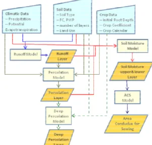
modified to derive the soil water status in the top layer (top 30 cm) of the soil profile. This is a simple book keeping-bucket type-water tight model which is based on law of conservation of mass. The basic assumptions of the model are i) the effective rainfall on any day is redistributed instantaneously and uniformly over the root zone, ii) The abstraction from the soil is also uniform through the entire root zone, iii)The runoff, deep percolation and evapotranspiration are sinks, iv) Since we are considering the early stage of the cropping season no interception losses are considered, v) Agriculture land are prepared and ready for sowing before the start of the season and vi) only the un-irrigated rainfed agricultural area are considered. Figure 1 presents the overview of the soil water balance model.
Figure 1: Overview of the soil water balance model This model considers the initial root depth of 30 cm through out the season to capture the soil water scenario for crops sown and germinating during any part of the cropping season. The soil water balance in the upper layer is governed by daily values of rainfall, runoff, evapotranspiration (ET) and drainage to the second layer. When the upper layer saturates in excess of Field Capacity (FC) due to rainfall, the excess water percolates to the lower passive root zone and are instantaneously redistributed in that zone. The excess soil water in the passive zone, moves out as deep percolation. Since the upper 30 cm is considered for the soil water assessment, the lower limit of soil water is the residual water content of the soil as the upper layer is exposed to the atmosphere and subjected to upward flux due to the direct solar radiation. The components of a generic hydrological model include rainfall, runoff, infiltration, evapotranspiration, percolation and deep percolation. Each of the components are described here under.
2.2.2 Potential Evapotranspiration: The daily global Potential Evapotranspiration (PET) data was downloaded from http://earlywarning.usgs.gov/fews/global/ web/dwnglobalpet.php web page. The daily PET is calculated from climate parameter data that is extracted from NOAA, Global Data Assimilation System (GDAS) analysis fields. The daily PET is calculated on a spatial basis using the Penman-Monteith equation (the formulation of Shuttleworth (1992) for reference crop evaporation is used). The data was downloaded and imported through appropriate software and sub-sampled to 1 km x 1 km resolution. Since this study deals with the early crop stages, the initial stage crop coefficient (Kc ) was adopted using the dual Kc approach proposed by Allen et al. (1998) which is defined by
ETc = (Kcb + Ke) ETo (3) Where Kcb - basal crop coefficient (0.15)
Ke – is the soil evaporative coefficient.
The Ke varies from 0.15 to 1.15 depending on the antecedent soil moisture condition. If the soil is dry Ke takes the lower value towards 0.15 and if the soil is wet it takes the higher value towards 1.15
2.2.3 Top Layer Soil Moisture (ș1
i ): The top 30 cm soil layer is the initial stage root depth for most of the crop. The soil moisture in the top layer is very critical in the sowing, germination and establishment of the crop. The top layer soil moisture is derived at the end of each day using the daily soil water balance equation which is given by
ș1i = (ș1i-1 x RD i-1 + Ri - Qi - Pi - ETi ) / RDi (4) for i _ 1, 2,...N,
Where Ĭ1
i - Top layer soil moisture (m³/ m³) RD - the root depth (mm) during the initial stage R - rainfall (mm)
Q - runoff (mm)
Pi - percolation out of the top layer (mm) ET - evapotranspiration (mm/day) N - the number of days in the crop season
2.2.4 Runoff: Daily runoff (Q, mm) was estimated from spatial rainfall data using the USDA Soil Conservation Service (SCS, 1985) Curve Number (CN) technique with appropriate modification for Indian conditions based on Ministry of Agriculture (1972) & Sahu (1990) with respect to soil type. The soil information was derived from the 1: 1 million scale soil map which has three textural classes namely sandy, loamy and clayey. The parameter like the Field Capacity (FC) and the Permanent Wilting Point (PWP) were derived for each textural class using the Saxton et. al. soil triangle.
The values of the CN vary with Antecedent Moisture Conditions (AMC). AMCI, AMCII, and AMCIII, corresponds to dry, average, and wet catchment conditions, respectively. These conditions are identified empirically based on the cumulative rainfall of the 5 preceding days. If this rainfall is < 36.6 mm, then AMCI applies; if it is more than 53.3 mm, AMCIII applies; and if it is in between, AMCII applies. For soil regions of India except for the black soil region with AMCII and AMCIII condition the runoff is given by:
Q = (R - 0.3S)²/(R + 0.7S), if R > 0.3S (5)
Q = 0, if R <= 0.3S
And for black soil regions with AMCII and AMCIII conditions.
Q = (R - 0.1S)²/(R + 0.9S), if R > 0.1S (6) Q = 0, if R <= 0.1S
Where
S = 254(100/CN - 1) (7)
The values of the CN for average AMC (CN for AMCII or CN = CN2) are tabulated for various soil, land use, and management conditions by the Ministry of Agriculture (1972). The corresponding values of CN for dry CN1 and wet CN3 catchment conditions are given by:
CN1 = CN2 - {20(100 - CN2)/[100 - CN2 + exp(2.533 - 0.0636(100 - CN2))]} (8)
CN3 = CN2 exp[0.00673(100 - CN2)] (9)
2.2.5 Percolation (Pi ): Percolation is the amount of water that leaves the upper soil layer and enters the bottom passive root zone. Percolation is given by
Pi = Ri - Qi - (FC - ș1 i-1) RD i-1 (10) If Pi < 0, then Pi = 0 For the passive root zone,
2.2.6 Passive Layer Soil Moisture (ș2i ): It is the soil moisture
that is present in the bottom layer of the passive root zone which is 90 cm in this study. The bottom layer soil moisture is derived by:
if Pi = 0 ș2i = ș2 i-1 Otherwise, (11) ș2i = ș2
i-1 + Pi / (RDM - RDi) - DPi (12)
Where RDM is the maximum root depth (mm) and DP is the drainage out of the passive root zone layer (bottom layer) as deep percolation.
2.2.7 Deep Percolation (DPi): Deep percolation is the amount of water that leaves the bottom soil layer and enters the soil beyond the root zone. Deep percolation is given by
DPi = Pi - (FC - ș2
i-1) (RDM - RDi) (13) If DPi < 0 then DPi = 0
The SWB model was developed using the Spatial Modeler module of the ERDAS Imagine software. The model was run on a daily time step basis.
2.3 Area Conducive for Sowing (ACS)
known that the germination is maximum, if the soil moisture is any where between 50% to 80% of the FC. This study considers soil moisture above 60% of FC for a continuous period of 7 days as conducive for sowing. The soil moisture is continuously monitored for this condition from June with a moving window of 7 days to find out the area conducive for sowing.
3.0 RESULTS AND DISCUSSION
3.1 Identification of soil liquid water content increase due to rainfall using LSWI
Sowing of crops starts immediately after the first significant shower of the monsoon. If there is delay in monsoon, the sowing is also delayed. The information on commencement of crop season enables estimation of crop phenology, which in turn, is useful for estimation of crop water requirement. Hence it is imperative to know the increase in soil humidity due to onset of monsoon which initiates the sowing process. To identify the increase in soil liquid water content the Rate of Increase (RoI) of LSWI from one fortnight to the subsequent fortnight was computed for the two states under study for 2010. Figure 2 shows the fortnightly increase of LSWI and NDVI from the previous fortnight for 2010, for few typical districts of AP and TN.
Figure 2: RoI of LSWI and NDVI for few typical districts of AP and TN during 2010
It can be observed that the increase of LSWI from the first fortnight to second fortnight of June was more than 100% in most of the districts. In almost all the districts, the first to second fortnight increase is the largest increase of LSWI in the entire season. This clearly demonstrates that the LSWI is able to pick the increasing liquid water content in the soil following the onset of monsoon. Ananthpur and East Godavari has the largest increase of LSWI during June 1st to 2nd fortnight. In Ananthpur the RoI is close to 100 only as this districts has coarse textured soil which does not hold sufficient top soil moisture to reflect in
LSWI. The RoI of East Godavari was seen at 200 indicating the commencement of monsoon. These two districts received excess rainfall in first two fortnights of June. The district of Karimnagar which lies in the Telengana region received deficient rainfall during June but received normal to excess rainfall in July. This was clearly picked up by LSWI by exhibiting maximum increase during July.
In TN the northern district of Kanchipuram and the delta district of Tiruvarur which received excess rainfall during June showed maximum increase of LSWI during the June 1st to 2nd fortnight. These districts also exhibited maximum increase of LSWI during the October 2nd fortnight to November 1st fortnight. This increase indicates the commencement of northeast monsoon in these districts. The southern district of Tuticorin which is influenced only by the northeast monsoon, show largest increase of LSWI only during November. In all these districts the NDVI did not show appreciable RoI when compared to LSWI during sowing window. Since NDVI is a vegetation index it showed no increase, since vegetation responds to rainfall with a lag of more then one fortnight. Further, wet soil after rainfall decreases the NIR reflectance thus reducing the NDVI.
3.2 Temporal Variations of Soil Moisture Index
Figure 3 gives the soil moisture index at the end of each month starting June to November 2010. The Soil Moisture Index (SMI) is defined as the proportion of the difference between the current soil moisture and the permanent wilting point to the field capacity and the permanent wilting point. The index values range from 0 to 100 with 0 indicating dry condition and 100 wet conditions. This figure also explains the dynamics of the soil moisture through the summer cropping season and start of winter cropping season in the top 30 cm soil layer. After the onset of monsoon the northern AP and TN districts were having good soil moisture. As the monsoon progressed during July and August almost all the district in AP and most of the districts in TN except for southern three districts were having sufficient top soil moisture. In September, the soil moisture reduced as the south west monsoon weaned. Due to the receipt of north east monsoon in October the coastal AP and entire TN got good rainfall resulting in sufficient soil moisture. During November TN continued to get the northeast monsoon rainfall and sustained its soil moisture while AP showed decrease in soil moisture.
To validate the soil moisture derived from the model, soil samples which were collected during October, November and December for an ongoing experiment in Guntur district was used. The field soil moisture was estimated using gravimetric method. The soil moisture predicted by the SWB model was regressed with observed sample soil moisture. Figure 4 gives the scatter plot which explains the relation between the SWB soil moisture and the sample soil moisture.
3.3 Area Conducive for Sowing
The condition for ACS was verified for every seven days window from the month of June till November. The ACS was aggregated for every fortnight which is co-terminus with the MODIS VI product time scale. Figure 5 gives the earliest period of attaining the ACS in different parts of AP and TN during June to November. Due to the timely onset and good amount of rainfall received during June and July most of AP became conducive for sowing by July. In TN, the north western districts of the state had ACS during June due to southwest monsoon. The north coastal districts became conducive for sowing during July and August. However the south eastern districts of Ramanathapuram, Tuticorin, Tirunelveli and part of Virudunagar became conducive for sowing only during the northeast monsoon period of October and November. Hence these districts can be classified as winter cropping season districts influenced only by northeast monsoon rainfall.
Jun Jul Aug
Sep Oct Nov Figure 3: Soil Moisture Index (SMI) of AP and TN at the end of
each month during 2010
Figure 4: Relation between the SWB soil moisture vs the observed soil moisture
3.4 Validation of ACS using LSWI
The model predicted ACS during a fortnight is the period when the soil in the district is wet (>60% FC) for continuous period of seven days. Under normal condition the sowing window for
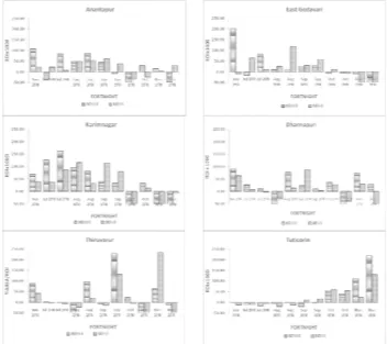
summer cropping season is between June to August and for winter cropping season, it is between October and November. The fortnightly district wise statistics of ACS confined to agriculture area was derived. To validate the ACS for each district, the percentage agriculture area under ACS was compared with the Rate of Increase (RoI) of LSWI between two successive fortnights. RoI of LSWI from one fortnight to the subsequent fortnight helps in identifying the increase in soil and vegetation liquid water content (Chandrasekar et. al., 2010). Figure 6 show the bar chart of fortnightly increase of LSWI along with percentage area of ACS, for few typical districts of AP and TN.
Figure 5: Earliest period of attaining the ACS in different parts of AP and TN during June to November 2010
Figure 6: ACS (%) and RoI of LSWI for few typical districts of AP and TN during June to November 2010
fortnight and simultaneously the RoI was also maximum during that fortnight. Tiruvarur district of TN is an irrigated district. Hence, it can be observed that the higher RoI of LSWI was seen during the second fortnight of June indicating the commencement of the season due to irrigation though there is no ACS area due to rainfall. Another increase of RoI of LSWI was seen in September indicating the commencement of rabi crop in the district. Tuticorin which is influenced by the northeast rainfall showed largest district RoI of LSWI during November 2nd fortnight which coincided with the majority of its district area becoming ACS.
4.0 CONCLUSION
Information on the sown area during the early crop season, is critical for early season agricultural drought management. First part of this study analysed the sensitivity of the LSWI and NDVI to the onset of monsoon and subsequent increase of soil humidity and vegetation water content. The RoI of LSWI and NDVI from one fortnight to the subsequent fortnight was computed. The RoI of LSWI was the highest during the fortnights when the onset of monsoon occurred. On the contrary the NDVI was stable or decreased in some cases during these fortnights due to low vegetative cover and wet soil background. The above observation showed that LSWI is sensitive to the onset of monsoon and initiation of cropping season.
The second part of this study has attempted to derive this information on ACS for the districts of AP and TN from June to November 2010, through the development of a simple soil water balance model. The model provides the top 30 cm profile soil wetness by using spatial inputs like the rainfall, PET, soil and crop parameter. The predicted soil moisture of the model was regressed with the ground observed soil moisture, which revealed the coefficient of determinant (r²) of 0.714.
The modeled soil moisture was used to derive the ACS over the states. The fortnightly ACS for each district was derived. It was clear from the observations that when ever more than 50% of a district area attains ACS for the first time during the sowing window, the RoI of LSWI was also the largest for the season indicating the commencement of the cropping season. The observations also clearly indicated that the soil wetness derived ACS was informative on the temporal variations in the start of the cropping season across the districts.
REFERENCES
Allen, R.G., Pereira, L., Raes, D. & Smith, M. 1998. Crop Evapotranspiration. Food and Agriculture Organization of the United Nations, Rome, Italy. FAO publication Vol.56. ISBN 92-5-104219-5. 290p.
Bannari, A., Morin, D., Bonn, F. and Huete, A.R. 1995. A review of vegetation indices. Remote Sensing Review. Vol.13, pp. 95-120.
Behrenfeld, M. J., Randerson, J.T., McClain, C.R., Feldman, G.C., Los, S. O., Tucker, C.J., Falkowski, P.G., Field, C.B., Frouin, R., Esaias, W.E., Kolber, D.D., and Pollack, N. H. 2001. Biospheric Primary Production During an ENSO Transition. Science, Vol 291, pp. 2594 – 2597.
Chandrasekar, K. , Sesha Sai, M. V. R. , Roy, P. S. & Dwivedi, R. S. 2010. Land Surface Water Index (LSWI) response to rainfall and NDVI using the MODIS Vegetation Index product. International Journal of Remote Sensing, Vol.31: 15, pp. 3987-4005.
Gao, B. C. 1996. NDWI-A normalized difference water index for remote sensing of vegetation liquid water from space. Remote Sensing of Environment, Vol.58, pp. 257-266.
Hojin K., Huete, A.R., Pamela N, Ed Glenn, William Emmerich and Russell L. Scott. 2004. Monitoring riparian and semi-arid upland vegetation using vegetation and water indices from the MODIS satellite sensor. Research insights in semiarid ecosystems (RISE). Symposium, 13th November, 2004, University of Arizona, Tucson, Marley Building.
http://disc2.nascom.nasa.gov/Giovanni/tovas/realtime.3B42RT_d aily.shtml (accessed 28 Sep. 2010)
Mandal U. K, Sundara Sarma, K. S., Victor, U. S. & Rao, N. H. 2002. Profile Water Balance Model under Irrigated and Rainfed Systems. Agronomy Journal, Vol. 94, September–October. Ministry of Agriculture. 1972. Handbook of hydrology. Government of India, New Delhi.
Mishra, P.K. 2005. Guidelines for rainfed production system and management, Drought Management, edited by K.D. Sharma and K.S Ramasastri, (Allied Publishers Private Limited), pp. 387-398. Running, S.W., Thornton, P.E., Nemani, R., & Glassy, J.M. 2000. Global terrestrial gross and net primary productivity from the Earth Observing System. In Methods in ecosystem science, Eds: Sala, O.E., Jackson, R.B., Mooney, H. A., & Gowarth, R.W. Springer, New York, pp. 44-57.
Sahu, D. 1990. Land forms hydrology and sedimentation. Naya Prakash Publ., Calcutta, India.
Shuttleworth,W.J. 1992. Evaporation. In D. Maidment, Handbook of Hydrology. McGraw-Hill.
Tucker, C.J.1980. Remote sensing of leaf water content in the near infrared. Remote Sensing of Environment, Vol.10, pp.23-32. Vermote, E. F., Saleous, N. Z., and Justice, C. O., Kaufman, Y. J., Privette, J., Remer, L., Roger, J. C., & Tanre, D. 1997. Atmospheric correction of visible to middle infrared EOS-MODIS data over land surface, background, operational algorithm and validation. Journal of Geophysical Research, 102(14), pp. 17131-17141.
Xiao, X., Zhang, Q., Braswell, B., Urbanski, S., Boles, S., Wofsy, S. C., et al., 2004. Modeling Gross primary production of a deciduous broadleaf forest using satellite images and climate data. Remote Sensing of Environment, Vol.91, pp.256 - 270.
ACKNOWLEDGMENTS