arXiv:0806.4666v1 [math.DG] 29 Jun 2008
On the Index of Constant Mean Curvature 1 Surfaces in
Hyperbolic Space
Levi Lopes de Lima, Wayne Rossman Department of Mathematics Universidade Federal do Cear´a
Fortaleza, Brasil June 29, 2008
Abstract
We show that the index of a constant mean curvature 1 surface in hyperbolic 3-space is completely determined by the compact Riemann surface and secondary Gauss map that represent it in Bryant’s Weierstrass representation. We give three applications of this observation. Firstly, it allows us to explicitly compute the index of the catenoid cousins and some other examples. Secondly, it allows us to be able to apply a method similar to that of Choe (using Killing vector fields on minimal surfaces in Euclidean 3-space) to our case as well, resulting in lower bounds of index for other examples. And thirdly, it allows us to give a more direct proof of the result by do Carmo and Silveira that if a constant mean curvature 1 surface in hyperbolic 3-space has finite total curvature, then it has finite index. Finally, we show that for any constant mean curvature 1 surface in hyperbolic 3-space that has been constructed via a correspondence to a minimal surface in Euclidean 3-space, we can take advantage of this correspondence to find a lower bound for its index.
1
Introduction
In a seminal paper [By], R. Bryant has shown that the geometry of surfaces with constant mean curvature 1 in hyperbolic 3-spaceH3(−1) has many similarities with the geometry of minimal surfaces in Euclidean spaceR3. It was shown in particular that such surfaces admit a Weierstrass representation in terms of certain holomorphic data (see section 3 below for details). A detailed analysis of this representation has allowed the construction of many complete examples ([UY1], [RUY]).
to Fischer-Colbrie [FC], who has shown that a minimal surface in R3 has finite index if and only if its total curvature is finite. (In regard to this, see also [G].) In fact, Fischer-Colbrie’s analysis allows us to obtain explicit estimates for the index of concrete examples with finite total curvature. Recall that any such surface is conformally equivalent to a compact Riemann surface Σ punctured at finitely many points corresponding to the ends of the original surface. Moreover, the Gauss map ofM extends meromorphically across the punctures defining a meromorphic mapg: Σ→S2. Then, it follows from Fischer-Colbrie’s
arguments that the index of M coincides with the index of the Schr¨odinger operator on Σ defined by
L=△ − |dg|2 .
Here,△and|dg|are computed relatively to any metric on Σ that is conformally equivalent to the original metric on M.
The purpose of this paper is to extend this circle of ideas to constant mean curvature 1 surfaces in H3(−1). In this case, the role played by the map g is replaced by the so-called secondary Gauss map G(we describeG below; it is a certain multivalued map that comes from the Bryant-Weierstrass representation). It so happens that ifM ∈H3(−1) has constant mean curvature 1 and finite total curvature, then M is also conformally finite, but it isnolonger true, in general, that Gextends meromorphically across the ends. This means, as we shall see, that the analysis necessary for studying the index in the H3(−1) case is much more involved than in theR3 case. More precisely, let ds2 and K denote the
induced metric and the Gaussian curvature in both cases. A common feature here is that K ≤ 0 and vanishes only at isolated points (unless M is either a plane or a horosphere) and thatd¯s2=−Kds2is a spherical pseudo-metric onM with conical singularities at these points.
A crucial point here is to determine the behavior ofd¯s2 at an end of M. To this effect,
let z = (x, y) be a conformal parameter around some end so that the end corresponds to z = 0. Note that, since M is complete, ds2 certainly becomes infinite when z → 0. Also, since the surface has finite total curvature, the limiting value of−K asz→0 is zero. So at first sight, it is unclear what the behavior ofd¯s2 =−Kds2 is at the ends. It is well known,
however, that in the minimal case we can choosez so that
d¯s2 = 4|g
′|2
(1 +|g|2)2|dz| 2 ,
where primes denote derivative with respect toz. Moreover, since g extends meromorphi-cally across the ends, we can assume g ≈ zℓ, ℓ ∈ Z+, so that d¯s2 is bounded around the end. One can now take advantage of this fact when one does the analysis necessary for examining the index of the minimal case, eventually obtaining Fischer-Colbrie’s results. In the hyperbolic case, we shall compute below that
d¯s2 = 4|G
′|2
(1 +|G|2)2|dz| 2 .
But now we can only assume thatG(z)≈zµ, for someµ >0 depending only upon the end. In particular, if 0< µ <1 for some end, d¯s2 isnotbounded at this end and the analysis for the minimal case does not apply to this situation.
¯
H1=H1
d¯s2 iscompactly embedded inL2ds¯2 (Lemma 4.4). Once this has been established, it
is an easy matter to use standard variational methods to define Ind(Σ) as being the index of a certain operator ¯L defined on Σ and corresponding to the Schr¨odinger operatorL in the minimal case (section 5). It follows easily from the construction that Indu(M) ≤ Ind(Σ),
where Indu(M) denotes the unconstrainedindex of M, namely, the index as computed for
not necessarily volume preserving variations (it follows from our arguments that Ind(M) and Indu(M) differ at most by 1, so that computing Indu(M) takes us a great deal of the way
toward computing Ind(M), our ultimate concern here). Furthermore, using standard results in elliptic regularity theory, we show that the eigenfunctions of ¯Lextend continuously across the ends (Lemma 5.2). This extra regularity property enables us to show that Ind(Σ) ≤ Indu(M), after an argument due to Fischer-Colbrie (Lemma 5.3).
Once this analysis is done, we find that we have an alternate proof of the result by do Carmo and Silveira [CS] that if a constant mean curvature 1 surface in H3(−1) has finite total curvature, then it has finite index (Corollary 5.2). The advantage of our way of proving this result is that it gives us tools that allow us to compute explicit bounds on index for some concrete examples. For some surfaces we can even compute the index exactly.
For example, using methods similar to those of Nayatani [N1], we can compute the index of the catenoid cousins and the Enneper cousins of higher winding order, as well as some other examples described by Umehara and Yamada [UY1] (section 6). Our results about the index of these examples yields some surprising differences from the index of minimal surfaces in R3. For example, unlike the minimal catenoid in R3, the catenoid cousins in H3(−1) can have arbitrarily high index (Theorem 6.1). Also, although the only minimal surfaces in R3 with index 1 are the catenoid and Enneper’s surface, there are many more examples of index 1 surfaces in the hyperbolic case (final remark of section 6).
As another example, using methods similar to those of Choe [Cho], we can compute lower bounds for many constant mean curvature 1 surfaces inH3(−1) (Theorem 7.1). We find lower bounds for genus 1n-noid cousins (Corollary 7.3), and for genuskCosta surface cousins (Corollary 7.1). And, in general, for those constant mean curvature 1 surfaces that are constructed via a deformation method [RUY] from minimal surfaces inR3, we can find a lower bound for index (Theorem 8.1).
The second author owes special thanks to Shin Nayatani for many helpful discussions. Thanks are also due to Pierre Berard, Etienne Sandier, Shin Kato, and David Goldstein.
2
Definition of index
Let Φ : M → M3(a) be an isometric immersion of a 2-dimensional manifold M into a complete simply-connected 3-dimensional manifoldM3(a) with constant sectional curvature a. Let N~ be a unit normal vector field on Φ(M) (we write Φ∗N~ simply as N~ defined on M). Let Φ(t) be a smooth variation of immersions fort∈(−ǫ, ǫ) so that Φ(0) = Φ. Assume that the variation has compact support. We can assume that the corresponding variation vector field at timet= 0 is u ~N, u ∈C0∞(M). Let A(t) be the area of Φ(t)(M) and H be the mean curvature of Φ(M). The first variational formula ([L]) is
dA dt
t=0
=−
Z
where h,i and dA are the metric and area form on M induced by the immersion Φ. If H is constant, then A′(0) = −nHRMudA. Let V(t) be the volume of Φ(t)(M), then V′(0) =RMudA. A variation is said to bevolume preserving ifRMudA= 0. It follows that Φ(M) is critical for area amongst all volume preserving variations.
The second variation formula for volume preserving variations ([Che], [Si], [L]) is
d2A dt2
t=0:=
Z
M{|∇
u|2−2(2a+ 2H2−K)u2}dA ,
whereKis the Gaussian curvature onM. Since we will be investigating surfaces of constant mean curvature 1 in hyperbolic space with constant sectional curvature−1, we will restrict ourselves to the casea=−1 and H= 1, so
d2A dt2
t=0
=
Z
M{|∇u|
2+ 2Ku2
}dA .
This formula is the same for both minimal surfaces in R3 := M3(0) and constant mean curvature 1 surfaces inH3:=M3(−1), giving us our first indication of the close relationship
between these two types of surfaces. Another indication of this close relationship is the Weierstrass representations described in the next section.
The index Ind(M) is the maximum possible dimension of a subspace of volume preserv-ing variation functions in C∞
0 (M) on which d
2A
dt2
t=0 <0. The purpose of this paper is to
estimate Ind(M).
We define Indu(M) as the maximum possible dimension of a subspace of (not necessarily
volume preserving) variation functions in C0∞(M) on which the above ddt2A2
t=0 <0. (The
subscriptu stands for “unconstrained index”.) Clearly, Indu(M) ≥ Ind(M). We will show
later that also Indu(M) −1 ≤ Ind(M). The methods we use in this paper allow us to
compute Indu(M), but what we really want to compute is Ind(M). However, these two
indices can differ by at most 1, so computing Indu(M) means that we know Ind(M) must
be either Indu(M) or Indu(M)−1.
3
The Weierstrass representation
Both minimal surfaces inR3and constant mean curvature 1 surfaces inH3 can be described parametrically by a pair of meromorphic functions on a Riemann surface, via a Weierstrass representation. First we describe the well-known Weierstrass representation for minimal surfaces in R3. We will incorporate into this representation the fact that any complete minimal surface of finite total curvature is conformally equivalent to a Riemann surface Σ with a finite number of points{pj}kj=1⊂Σ removed ([O]):
Lemma 3.1 Let Σ be a Riemann surface. Let {pj}kj=1 ⊂Σ be a finite number of points,
which will represent the ends of the minimal surface defined in this lemma. Let z0 be a
fixed point in Σ\ {pj}. Let g be a meromorphic function from Σ\ {pj} to C. Let f be a
holomorphic function from Σ\ {pj} to C. Assume that, for any point in Σ\ {pj}, f has
assume thatf has no other zeroes on Σ\ {pj}. Then
Φ(z) =Re
Z z
z0
(1−g2)f dζ i(1 +g2)f dζ
2gf dζ
is a conformal minimal immersion of the universal coverΣ\ {gpj}of Σ\ {pj}intoR3.
Fur-thermore, any complete minimal surface with finite total curvature inR3 can be represented
in this way.
The mapgcan be geometrically interpreted as the stereographic projection of the Gauss map. The first and second fundamental forms and the intrinsic Gaussian curvature for the surface Φ are
ds2= (1 +g¯g)2f dz·f dz , II =−2Re(Q), K =−4
|g′|
|f|(1 +|g|2)2
2
,
where the Hopf differentialQis defined to be Q=g′f dz2.
To make a surface of finite total curvature (i.e. RΣ−KdA <+∞, which is necessary to make a surface of finite index [FC]) we must choose f and g so that Φ is well defined on Σ\ {pj} itself. Usually this involves adjusting some real parameters in the descriptions of
f and g and Σ\ {pj} so that the real part of the above integral about any nontrivial loop
in Σ\ {pj} is zero.
We now describe a Weierstrass type representation for constant mean curvature c sur-faces inH3(−c2) :=M3(−c2). This result is a composite of several results that are found in [By], [UY3], [UY4].
Lemma 3.2 Let Σ, Σ\ {pj}, z0, f, and g be the same as in the previous lemma. Choose
a null holomorphic immersion F :Σ\ {gpj} →SL(2,C) so thatF(z0) is the identity matrix
and so that F satisfies
F−1dF =c g −g2 1 −g
!
f dz , (3.1)
then Φ :Σ\ {gpj} →H3(−c2) defined by
Φ = 1 cF
−1F−1t (3.2)
is a conformal constant mean curvature c immersion into H3(−c2) with the Hermitean
model. Furthermore, any constant mean curvature c surface with finite total curvature in
H3(−c2) can be represented in this way.
the sphere at infinity to the complex planeC[By]. The first and second fundamental forms and the intrinsic Gaussian curvature of the surface are
ds2 = (1 +GG)¯ 2f g
′
G′
f g′
G′
dzdz , II =−2Re(Q) +c ds2 , K =−4 |G
′|2
|g′||f|(1 +|G|2)2
!2
,
where in this case the Hopf differential isQ=−f g′dz2 (the sign change inQ is due to the fact that we are considering the “dual” surface; see [UY4] for an explanation of this), and whereGis defined as the multi-valued meromorphic function
G= dF11 dF21
= dF12 dF22
on Σ\ {pj}, with F = (Fij)i,j=1,2. The reason that G is multi-valued is that F itself can
be multi-valued on Σ\ {pj}(even if Φ is well defined on Σ\ {pj} itself). The functionGis
called thesecondary Gauss map of Φ ([By]).
In the above lemma, we have changed the notation slightly from the notation used in [By] and [RUY], because we wish to use the same symbol “g” both for the map g used in the Weierstrass representation for minimal surfaces inR3and for the hyperbolic Gauss map used in the Weierstrass representation for constant mean curvature surfaces in H3. And we further wish to give a separate notation ”G” for the secondary Gauss map used in the hyperbolic case. We do this to emphasize that, in relation to their geometric interpretations, the “g” in the Euclidean case is more closely related to the hyperbolic Gauss map “g” in theH3 case than to the secondary Gauss map “G” (as we will see in section 6).
In order for Φ to be well-defined on Σ\ {pj}itself, it is sufficient and necessary that F
satisfy a condition called theSU(2)-condition. Note that if one travels about a nontrivial loop in Σ\ {pj}, then F → BF, where B ∈ SL(2,C). If for every loop in Σ\ {pj}, the
resulting matrixBsatisfiesB∈SU(2), then theSU(2)-condition is satisfied. IfB ∈SU(2), thenF−1F−1t= (BF)−1(BF)−1t, so it follows that if theSU(2)-condition holds, then Φ is
well defined on Σ\{pj}itself. WhenF →BF, we have the following effect on the secondary
Gauss map:
G→ b11G+b12 b21G+b22
, forB = b11 b12 b21 b22
!
∈SU(2).
We now state some known facts, which when taken together, show that constant mean curvature 1 surfaces inH3 and minimal surfaces inR3 are very closely related. These facts provide the motivation for the results in sections 7 and 8 of this paper:
• It was shown in [UY2] that if f and g and Σ\ {pj} are fixed, then as c → 0, the
constant mean curvature c surfaces Φ in H3(−c2) converge to a minimal surface in
R3. This can be sensed from the fact thatG→g and B → identity as c→0 (which follow directly from equation 3.1), and hence the above first and second fundamental forms for the constant mean curvaturecsurfaces Φ converge to the fundamental forms for a minimal surface asc→0 (up to a sign change inII – a change of orientation).
surface inH3(−c2) forc≈0, so that Σ,f, andgare the same, up to a slight adjustment
of the real parameters that are used to solve the period problem. The deformed surface might not have finite total curvature, but it will be of the same topological type as the minimal surface, and it will have the same reflectional symmetries as the minimal surface.
• Consider the Poincare model forH3(−c2) forc≈0. It is a round ball in R3
centered at the origin with Euclidean radius 1c endowed with a complete radially-symmetric metricds2c = 4
P
dx2
i
(1−c2Px2
i)2
of constant sectional curvature−c2. Contracting this model
by a factor ofc, we obtain a map to the Poincare model forH3. Under this mapping, constant mean curvaturecsurfaces are mapped to constant mean curvature 1 surfaces. Thus the problem of existence of constant mean curvaturec surfaces in H3(−c2) for
c≈0 is equivalent to the problem of existence of constant mean curvature 1 surfaces in H3. Furthermore, under this mapping, the area form on the constant mean curvature c surface is changed only by a constant factor c2: If dA
c is the area form on the
constant mean curvature c surface, and dA1 is the area form on the constant mean
curvature 1 surface, then dAc = c2dA1. Hence a variation that reduces area on the
constant mean curvaturecsurface is mapped to a variation that reduces area on the constant mean curvature 1 surface (and vice-versa). Hence this mapping preserves the index.
4
Showing that
H
¯
1is compactly contained in
L
2ds¯2We now considerM to be a complete constant mean curvature 1 surface inH3 with finite total curvature. We will assume the surface is not a horosphere. (Assuming that the surface is not a horosphere will not add any extra conditions to our index results, since the index of the horosphere is known to be zero [Si].) Suppose thatM has Weierstrass representation Φ : Σ\ {pj} → M with Riemann surface Σ and functions f, g : Σ → C, and that G
is the secondary Gauss map. Let ds2 be the complete metric on M pulled back to Σ.
Note that M is conformally equivalent to Σ with a finite number of points {pj} removed;
each removed point pj corresponds to an end of M. So ds2 is defined on Σ\ {pj}. Let
d¯s2 = G∗ds2
S2 = −Kds2 be the singular pull back metric of the canonical metric on S2
via the secondary Gauss mapG, defined on Σ\ {pj}, but with isolated singularities where
K= 0. We letd˜s2 be a conformal nonsingular metric defined on Σ. Any choice ford˜s2 will suffice, provided it is conformally equivalent tods2 on Σ\ {p
j}. LetdA(resp. dA,¯ dA) and˜
∇ (resp. ¯∇, ˜∇) and △ (resp. ¯△, ˜△) be the area form and gradient and Laplacian on Σ with respect to the metricds2 (resp. d¯s2,d˜s2).
We choose the sign of the Laplacian so that RΩ|∇u|2 = +R
Ωu△u for anyu ∈C0∞(Ω).
(Thus, for example, the Laplacian on the standard Euclidean planeR2 will be−∂2 ∂x2 − ∂
2
∂y2.)
So if u ∈ C∞
0 (Ω) satisfies △u = λu for some constant λ, where Ω is a region in Σ, then
R
Ω|∇u|2 =
R
Ωu△u = λ
R
Ωu2 and so λ ≥ 0. Thus our convention for the sign of the
Laplacian implies that the eigenvalues of the Laplacian will be nonnegative.
We now list some easily determined facts that will be used throughout this and the next section. We can define|dG|2ds2(resp. |dG|2ds¯2,|dG|2d˜s2) by|dG|2ds2 =
P2
j=1hdG(ej), dG(ej)ids2
S2
(resp. |dG|2ds¯2 =
P2
j=1hdG(¯ej), dG(¯ej)ids2
S2
, |dG|2ds˜2 =
P2
j=1hdG(˜ej), dG(˜ej)ids2
S2
dG is the tangent map of G and {e1, e2} (resp. {e¯1,e¯2}, {˜e1,e˜2}) is an orthonormal basis
of vector fields with respect to the metricds2 (resp. d¯s2,d˜s2). The following hold:
• d¯s2=−Kds2,dA¯=−KdA,△=−K△¯
• d¯s2= 12|dG|d2s¯2d¯s2= 12|dG|2ds2ds2= 12|dG|2ds˜2d˜s2 (conformal invariance).
We now consider the variation described in the second section with variation vector field u ~N on M at time t = 0. Since ddt2A2
t=0 obviously depends on u, we will write it as
d2A
dt2
t=0(u). In the next lemma, we will consider Σ and u to be fixed, but we consider
whether or not ddt2A2
t=0(u) depends on G,g, and f.
We now state a crucial computation – it is crucial because it explains why the pull-back of the metric on the sphere via the mapGplays such a dominant role in computing Ind(M), and explains why the operatorsL and ¯L (defined later) are somehow “the same” operator:
d2A dt2 t=0 (u) = Z
Σ{|∇u|
2+ 2Ku2
}dA=
Z
Σ{u△u+ 2Ku 2
}dA=
Z
Σ{−uK
¯
△u+ 2Ku2}dA=
Z
Σ{−u
¯
△u+ 2u2}KdA=
Z
Σ{u
¯
△u−2u2}dA .¯
Since the integrand{u△¯u−2u2}dA¯is completely determined by the pull-back of the spher-ical metric via the map G, we know that ddt2A2
t=0(u) depends only on G, and does not
depend ong and f.
Lemma 4.1 ddt2A2
t=0(u) is completely independent of f and g. It does depend on G, but not on the choice of value of the multi-valued G.
Proof. As noted above, ddt2A2
t=0(u) depends only onG, not ongandf. Clearly,
d2A
dt2
t=0(u)
does depend on G, but to show that it does not depend on the choice of value of the multi-valuedG, we first show that the first fundamental form is independent of theSU (2)-condition. Let ˆf =−g′f /G′. Travelling about a loop in Σ corresponding to a homologically nontrivial loop in M, we have F → BF for some B ∈ SU(2), and as we saw before G → (b11G+b12)/(b21G+b22), where bij are the entries of B. Thus travelling about
the loop makes the transformation G′ → G′/(b21G+b22)2, and since f and g are left
unchanged (and therefore g′ is also unchanged), it follows that ˆf → f(bˆ 21G+b22)2. Now
we consider the conformal factor ˆffˆ(1 +GG)¯ 2)2 in the first fundamental form. Denoting (b11G+b12)/(b21G+b22) asB·G, we see that
ˆ
ffˆ(1 +GG)¯ 2)2 →(b21G+b22)2f(bˆ 21G+b22)2fˆ(1 + (B·G)(B·G))2= ˆff(1 +ˆ GG)¯ 2)2 ,
sinceb11=b22 and b12=−b21.
Thereforeh,i is independent of the SU(2)-condition, and therefore∇u anddAare inde-pendent of theSU(2)-condition, since they are determined by the first fundamental form. And since K depends only on the first fundamental form, K is also independent of the SU(2)-condition. We conclude that ddt2A2
t=0(u) is independent of the SU(2)-condition.
Thus ddt2A2
For any p ≥2, let Lpds˜2(Ω) (resp. Lpds¯2(Ω)) be the space of measurable functions f on
Ω⊂Σ such that RΩ|f(x)|pd˜s2dA <˜ ∞ (resp. R
Ω|f(x)|
p
ds¯2dA <¯ ∞). In the case that Ω = Σ,
we may write simplyLpds˜2 (resp. Lpd¯s2) instead of Lpd˜s2(Σ) (resp. Lpd¯s2(Σ)).
We now begin to work toward a proof that ¯H1 is compactly contained in L2
ds¯2.
Lemma 4.2 If p is sufficiently large, thenLpd˜s2 is continuously contained in both L2ds˜2 and
L2ds¯2.
Proof. Since Σ is compact, Lpd˜s2 is continuously contained in L2ds˜2 for all p≥2. (See, for
example, [GT], equation (7.8)).
As for the second assertion, consider a pointpj ∈Σ representing an end of the complete
surface. LetUj be a small neighborhood ofpj. We may choosed˜s2so thatd˜s2=dx2+dy2 =
4dzd¯z on Uj. We now show that locally onUj,
d¯s2 ≈4µ2 r
2µ−2
(1 +r2µ)2d˜s 2 ,
with r = px2+y2. (The symbol ”≈” means that for functions a(z), b(z) defined in a
neighborhood ofz = 0, a(z) ≈b(z) if for all ǫ > 0, there exists a δ > 0 such that |z|< δ implies|ab((zz))−1|< ǫ.) The above relation follows from the fact that locally near an end we can make the following normalization: we can choose the complex coordinatezonUj so that
the endpjis atz= 0. By the previous lemma, we may changeGto (b11G+b12)/(b21G+b22)
for anyB ={bij} ∈SU(2), without affecting the second variation formula. We may choose
B so that ((b11G+b12)/(b21G+b22))(z= 0) = 0. Hence we may assume that G(0) = 0. We
then have that G= zµG, where ˆˆ G is a holomorphic function in a neighborhood of z = 0 such that ˆG(0)6= 0, for someµ∈R+, wherez=x+iy[UY1]. Changingz to ˆG(0)−1/µzif
necessary, we may assume that ˆG(0) = 1.
The point corresponding to G(z) under the inverse of stereographic projection is
G= (G1,G2,G3) =
1
|G|2+ 1(2Re(G),2Im(G),|G| 2
−1) .
Note that for any real-valued function f : C → R, we have fz = 1
2(fx−ify), so |fz|2 = 1
4(|fx|2 +|fy|2). For any complex-valued holomorphic function f : C → C, we have
∂
∂z(Re(f)) = ∂z∂ 12(f+ ¯f) = 21fz, ∂z∂ (Im(f)) = ∂z∂ i2( ¯f−f) =−i2 fz, and ∂z∂(ff) =¯ fzf¯+ff¯z=
¯
f fz. Using these properties and the fact thatG=zµG, we haveˆ
|dG|2d˜s2 =|dG|2ds˜2 =
3
X
i=1
|∇Gi|2 =
3
X
i=1
(|(Gi)x|2+|(Gi)y|2)
=
3
X
i=1
4|(Gi)z|2 =
8GzGz
(1 +GG)¯ 2 ≈
8µ2r2µ−2 (1 +r2µ)2 .
And thus it follows thatd¯s2 ≈4µ2(1+r2rµ2−2µ)2d˜s2 on Uj.
Supposeu∈Lpd˜s2(Uj). By the Holder inequality we haveRUju
2dA¯=R
Uju
2 1
2|dG|2d˜s2dA˜≤
A2pB1q, where A = R
Uju
pdA˜ and B < cR Ujr
(2µ−2)qdA, with˜ 2
finite constant. If q is close enough to 1, then B is finite, since µ > 0 and dA˜ has the local expressiondA˜ =rdrdθ in polar coordinates. So there exists a constant kj such that
||u||L2
ds¯2(Uj)≤
kj||u||Lp
d˜s2(Uj)
for eachj.
On Σ\ {∪Uj},d¯s2is bounded. So it is clear from the Holder inequality that there exists
a constantk0 such that||u||L2
ds¯2(Σ\{∪Uj}) ≤
k0||u||Lp
ds˜2(Σ\{∪Uj})
. Let k= max{k0, kj}. Then,
choosingp large enough, we have ||u||L2
ds¯2 ≤
k||u||Lp ds˜2
. ✷
Remark. Ifµ≥1 for all ends, thend¯s2 is bounded on all of Σ, and the lemma holds even
forp= 2. We could argue this way: supposeu∈L2ds˜2. Then R
Σu2dA¯=
R
Σu2 12|dG|2d˜s2dA˜≤
(const)RΣu2dA. Thus˜ ||u||L2
d¯s2 ≤
(const)||u||L2
d˜s2
. SoL2d˜s2 is continuously included in L2ds¯2.
✷
We define ˜H1(Σ) ={u∈L2d˜s2 |du∈L2d˜s2}, where the derivativedu= (∂x∂u1,∂x∂u2) satisfies R
Σh∂x∂ui, φid˜s2d
˜
A = RΣhu,∂x∂φ
iid˜s2d
˜
A for all test functions φ ∈ C∞(Σ) and all coordinate
functions xi. The condition that du must satisfy depends on d˜s2, but it is well known
that ˜H1 is independent of d˜s2 if d˜s2 is a true metric and not a pseudometric. We define
¯
H1(Σ) ={u∈L2ds¯2 |du∈L2ds¯2}, wheredusatisfies R
Σh∂x∂ui, φid¯s2d
¯
A=RΣhu,∂x∂φ
iids¯2d
¯ Afor all test functionsφ∈C∞(Σ) and all coordinate functionsx
i. Note thatd¯s2 is a psuedometric
and might not be a true metric even away from the endspjof the surface, since the secondary
Gauss map may have branch points even at finite points on the surface. We define the two norms
˜
||u˜||2:=
Z
Σ
(|∇˜u|2ds˜2 +u2)dA˜
¯
||u¯||2:=
Z
Σ
(|∇¯u|2ds¯2 +u2)dA¯= Z
Σ
(|∇˜u|2d˜s2+
1 2|dG|
2
ds˜2u2)dA .˜
Lemma 4.3 H¯1 is continuously contained in H˜1.
Proof. We need to show that there exists ac >0 such that ˜|| ·˜|| ≤c¯|| ·||¯.
By way of contradiction, suppose that such accannot exist. Then there exists a sequence
{un}∞n=1 of functions such that ˜||un||˜= 1 and ¯||un¯||< n1. Note the following three facts:
• Any bounded sequence in a Hilbert space has a weakly convergent subsequence (see, for example, [GT], p85). In our case the Hilbert space is ( ˜H1,|| ·˜ ||˜).
• The inclusion of ˜H1 into Lpd˜s2 is compact for all p ∈[2,∞) (See, for example, [GT],
Theorem 7.22, or see [Ad].)
• ˜|| ·||˜ is lower semicontinuous with respect to weak convergence; that is, if un → u
weakly, then ˜||u˜|| ≤lim infn→∞||˜un||˜.
By the first fact, we may assume that{un}converges weakly in ˜H1 to someu∈H˜1. By the
second fact, we may assume that {un} converges strongly in L2ds˜2 to somev ∈L2d˜s2. Since
˜
H1 ⊂L2ds˜2 continuously, we have that un →u ∈L2ds˜2 weakly. And since the weak limit is
unique, we haveu=v. By the third fact, we have
Z
Σ(|
˜
∇u|2d˜s2+u2)dA˜≤lim inf
n→∞
Z
Σ(|
˜
We have strong convergence ofun to u inL2d˜s2, hence R
Σu2ndA˜→
R
Σu2dA. So we have˜
Z
Σ|
˜
∇u|2ds˜2dA˜≤lim inf
n→∞
Z
Σ|
˜
∇un|2d˜s2dA .˜
And then since RΣ|∇˜un|2ds˜2dA˜= R
Σ|∇¯un|2ds¯2dA <¯ n1, we have R
Σ|∇˜u|2d˜s2dA˜= 0. Therefore
u is constant almost everywhere. Since 1− n1 ≤RΣu2ndA˜≤ 1 we have RΣu2dA˜= 1 (Here again we are using thatun→ustrongly inL2d˜s2.) Thereforeuis equal to a nonzero constant
almost everywhere.
By the previous lemma, Lpds˜2 is continuously included in L2ds¯2 for p large enough. By
the second fact, ˜H1 is compactly contained in Lpds˜2, so it follows that ˜H1 is compactly
contained inL2ds¯2. This means that any weakly convergent sequence in ˜H1 (which is
there-fore a bounded sequence in ˜H1) has a strongly convergent subsequence in L2
ds¯2. So, since R
Σu2ndA¯ ≤ 1n, we have
R
Σu2dA¯ = 0. But u is a nonzero constant, so 0 =
R
Σu2dA¯ =
(const6= 0)·RΣ12|dG|2d˜s2dA. Therefore˜ |dG|ds˜2 = 0 almost everywhere, and thus |G′| = 0.
Hence K = −4 |G′|2/(|g′||f|(1 +|G|2)2)2 = 0, which implies the surface is umbilic, and
hence a horosphere. But we assumed the surface is not a horosphere, so this is a
contradic-tion. ✷
Remark. If µ≥1 for all ends of a constant mean curvature 1 surface M, then H˜1 = ¯H1.
We already know that ¯H1 is continuously included in ˜H1, so to show this it remains only
to show that there exists ac >0 such that ¯|| ·¯|| ≤c˜|| ·||˜. At points whereGis not branched we can make a local expression G=az+bz2+. . . with a6= 0. We may assumed˜s2 is the Euclidean metric locally, so|dG|ds˜2 =aat the chosen point . At points whereGis branched
we can make a local expression ¯G = azm +bzm+1 +. . . with a 6= 0 and m ∈ Z, m ≥ 2.
In this case |dG|ds˜2 = 0 at the chosen point. At each end we can make a local expression
G= zµ(a+bz+cz2+. . .) with a6= 0 and µ ≥1. In this case |dG|d˜s2 = 0 at the chosen
point ifµ >1, and|dG|ds˜2 =aat the chosen point ifµ= 1. In any case|dG|ds˜2 is bounded,
and the existence ofcfollows. ✷
Remark. Since d¯s2 is identically zero for the horosphere, the calculations in this section
would have no meaning for this example. And as it is the only example for which d¯s2 is zero at more than just isolated points, it is natural to exclude it. In any case, the index of
the horosphere is easily seen to be 0 (see section 6). ✷
Lemma 4.4 H¯1 is compactly contained inL2ds¯2.
Proof. H¯1 is continuously contained in ˜H1, and ˜H1 is compactly contained inLp
ds˜2 for any
value ofp, andLpds˜2 is continuously contained inL2d¯s2 ifpis large enough. The composition
of a continuous map and a compact map and a continuous map is compact. ✷
5
The relationship between Ind(
M
) and eigenvalues of
L
¯
The last lemma in the previous section will lead us to an argument that Ind(Σ) is equal to the number of negative eigenvalues of ¯L on Σ. (We are about to define Ind(Σ) and ¯L.) First we show that Rayleigh quotient Q (as defined in the next lemma) is well defined for any smooth function on Σ. This next lemma will allow us to start the minimization process (i.e. Q(u)<∞ for someu) in the proof of the lemma which comes after it.
Before considering the next lemma, we define the relevant Jacobi operators. The original Jacobi operator on M is L =△ − |dG|2ds2 =△+ 2K on Σ. The Jacobi operator created
by pulling back the metric on the sphere viaGis ¯L= −K1△ − |dG|2
ds¯2 = ¯△ −2 on Σ. Note
that ¯Lis defined everywhere on Σ except at the isolated points whered¯s2= 0 and possibly at points that represent the ends of M. The operator associated to the regular metric d˜s2 is ˜L= ˜△ − |dG|2
d˜s2, and is defined on all of Σ, except possibly at points that represent the
ends ofM. We have Z
Σu
˜ LudA˜=
Z
ΣuLudA=
Z
Σu
¯ LudA .¯
SinceL, ¯L, and ˜L are not well defined only at isolated points of Σ, these integrals are well defined.
Lemma 5.1 Q(u) :=
R
ΣuLud¯ A¯ R
Σu2dA¯
<∞ for all u∈C∞(Σ).
Proof. Locally at each end, we can normalize G(z) to be G = zµ(1 +a1z+a2z2 +. . .),
wherez is contained in a neighborhoodU ofz = 0, andz = 0 represents the end, andd˜s2
is the Euclidean metric on U, andµ >0, and |dG|2d˜s2 ≈
8µ2|z|2µ−2
(1+|z|2µ)2. (We showed this in the
proof of Lemma 4.2.) Since RΣuLud˜ A˜ = RΣuLud¯ A, we can show that the numerator of¯
Q(u) is finite by showing thatRΣuLud˜ A˜is finite. To show this, it is sufficient to show that
R
UuLud˜ A˜is finite at each end, sinceu∈C∞(Σ), andd˜s2 is nonsingular on the compact Σ,
and ˜Lis nonsingular on Σ away from the ends.
Sinceu∈C∞(Σ), we have thatu, ux, uy are all bounded onU. Sinced˜s2is the Euclidean
metric on U, we have that dA˜= rdrdθ in polar coordinates on U. Furthermore, we have µ >0, hence
Z
U u
2
x+u2y−
8µ2r2µ−2u2 (1 +r2µ)2
!
rdrdθ
<∞.
So the numerator ofQ(u) is finite, and therefore|Q(u)|<∞. ✷
Given any closed region Ω⊂Σ\ {pj}, we can consider the Dirichlet problemLu=λu
and ¯Lu=λu on Ω withu|∂Ω = 0. In general,Land ¯Lwill have different eigenvalues on Ω;
however, supposing that V is some vector space of functions with compact support on Ω,
Q(u)<0 for allu∈V if and only if
R ΩuLudA R
Ωu2dA
<0 for allu∈V. We define Ind( ¯L,Ω) to be the maximum possible dimension of a subspace of functions inC∞
0 (Ω) on whichQ(u)<0. We
define Ind(L,Ω) to be the maximum possible dimension of a subspace of functions inC0∞(Ω)
on which
R ΩuLudA R
Ωu2dA
< 0. Thus Ind( ¯L,Ω) = Ind(L,Ω). We consider a sequence of regions
{Ωi}∞i=1such that Ωi⊂Ωi+1and∪Ωi= Σ\{pj}. We define Ind( ¯L, M) = limi→∞Ind( ¯L,Ωi),
by the definition given in the second section, Indu(M) = Ind(L, M). Defining Ind(Σ) :=
Ind( ¯L,Σ) to be the maximum possible dimension of a subspace of functions in C∞(Σ) on whichQ(u)<0, we have
Indu(M)≤Ind(Σ).
In order to explicitly compute Indu(M) and to show that Indu(M) = Ind(Σ), we would
like to know that Ind(Σ) equals the number of negative eigenvalues of L¯ on Σ. That this holds (Corollary 5.1) can be concluded from the next lemma. The fact that Ind(Σ) equals the number of negative eigenvalues of ¯Lon Σ is very useful for making explicit estimates of Ind(M), as we shall see.
Lemma 5.2 We can find weak solutions u ∈ H¯1 of Lu¯ = λu on Σ so that the following
hold:
• The set of eigenvalues consists of an infinite sequence
λ1 < λ2< . . .→ ∞.
• Each eigenvalue has finite multiplicity and the eigenspaces (of weak solutions) corre-sponding to distinct eigenvalues are L2
d¯s2 orthogonal.
• The direct sum of the eigenspaces is dense inL2d¯s2 for the L2ds¯2 norm.
• Any eigenfunctionuof λj is contained inC∞(Σ\ {pj}) and satisfies Lu¯ =λju in the
classical sense onΣ\ {pj}.
• Any eigenfunction u of λj is contained in C0(Σ).
Proof. The Rayleigh-Ritz quotient as defined in Lemma 5.1 is
Q(u) :=
R
Σ|du|2ds¯2 −2u2dA¯ R
Σu2dA¯
=
R
Σ|du|2d˜s2 − |dG|2d˜s2u2dA˜ R
Σ 12|dG|2d˜s2u2dA˜
, u∈H¯1.
The denominator is theL2ds¯2 norm.
The proof of the first three items follows by standard variational arguments, such as in the arguments on pages 55-59 of [Be]. The only difference between the proof of the lemma above and the proof in [Be] is that elliptic regularity is used there to show that the eigenfunctions corresponding to the eigenvalues are classical solutions of the eigenvalue problem (on all of Σ). In our case we only conclude that we have weak solutions to the eigenvalue problem. However, we can simply ignore the arguments where elliptic regularity is used, and the remaining arguments in [Be] are sufficient to prove the first three items in the above lemma, so we shall not repeat the arguments here.
We remark that in order to apply these standard variational arguments, it is crucial that we know that ¯H1 is compactly included in L2
ds¯2. This is why we were focusing on proving
Lemma 4.4 in the previous section.
We now turn to proving the last two items in the lemma. Supposeuis a weak solution of ¯
Lu=λju, so ˜△u=quin the weak sense, whereq= (1+λ2j)|dG|2ds˜2. Sinceq∈C∞(Σ\{pj}),
it follows from elliptic regularity ([GT], Corollary 8.11) thatu∈C∞(Σ\ {pj}) and satisfies
¯
Consider a small neighborhood Uj ⊂ Σ of the point pj representing an end. Ifµj ≥ 1
at pj, then q ∈ C0(Uj), and therefore any eigenfunction u is contained in C0(Uj) ([GT],
Theorem 8.8 and Corollary 7.11). If µj <1 at pj, we will see in the next three paragraphs
thatu is still contained in C0(U
j).
To show u ∈ C0(Σ), we only need to show u ∈ C0(Uj), since u is C∞ away from
the pj. First we state theorem 17.1.1 from [H]. Consider a linear operator of order m,
P(x, D) = P|α|≤maα(x)Dα in an open set X ⊂ Rn. We may assume X = Uj, since we
may choose d˜s2 to be the standard Euclidean metric on Uj. In our case P(x, D) = ˜△,
m = n = 2. Suppose that Pm(0, D) = P|α|=maα(0)Dα is elliptic. This is certainly true
for ˜△. Suppose also that aα in continuous when |α|= m, and that for some r ∈ (1,∞),
aα ∈ L
n m−|α|
loc,ds˜2(Uj) if m− |α|< nr, andaα ∈Lloc,dr+ǫs˜2(Uj) for some ǫ >0 ifm− |α|= nr, and
aα ∈ Lrloc,ds˜2(Uj) if m− |α|> nr. In our case all of the coefficients are constant, so these
conditions will hold. The theorem says that if all these conditions are satisfied and Uj is
a sufficiently small neighborhood of pj, then there is a linear operator E inLrd˜s2(Uj) such
that
• f ∈ Lrds˜2(Uj) → DαEf ∈Lsd˜s2(Uj) is continuous if r ≤ s≤ ∞ and 1s ≥ 1r −(m−|α|n )
with strict inequality ifs=∞,
• P(x, D)Ef =f,f ∈Lr ds˜2(Uj),
• EP(x, D)v = v if v∈C∞
0 (Uj).
In our case we will have Ef =u and f =qu. We will choose 1< r=s≈1. We now show that qu ∈Lr
d˜s2(Uj) if r is sufficiently close to 1. Since u ∈ H¯1, Lemma
4.3 implies that u ∈ H˜1. And since ˜H1 is compactly contained in Lpd˜s2 for all p ≥2, we
have thatRU
ju
pdA˜is finite for all p≥2. As we saw in the proof of Lemma 4.2,R Ujq
tdA˜ is
finite ift(t >1) is sufficiently close to 1. Choose such a tsufficiently close to 1, and choose p sufficiently large so that 1p + 1t < 1. Define r > 1, r ≈1 by 1r = 1p +1t. By the Holder inequality, (RU
j(qu)
rdA)˜ 1r ≤(R Ujq
tdA)˜ 1t(R Uju
pdA)˜ 1p <∞.
So we have that qu ∈ Lr
d˜s2(Uj), and, by the theorem from [H] stated above, we have
that the mapf →DαEf from Lrds˜2(Uj) to Lsd˜s2(Uj) is continuous when|α| ≤2 and s=r.
Therefore, letting Ef =u and f =qu, we have||Dαu||Ls=r
d˜s2(Uj) ≤c||qu||L r
ds˜2(Uj) <∞ when |α| ≤ 2. This implies that u is contained in the Sobolev space W2,r(Uj). Then, since
u∈W2,r(U
j), we have u∈C0(Uj) (see, for example, [GT], Corollary 7.11). ✷
Corollary 5.1 Ind(Σ) = the number of negative eigenvalues (counted with multiplicity) of
¯ L on Σ.
This corollary follows immediately from the variational characterization of the eigenval-ues (for example, see [Be], p61). Thek’th eigenvalueλk is characterized by
λk= inf Vk
sup{Q(u)|u∈Vk, u6= 0},
whereVk runs through allkdimensional subspaces of ¯H1.
Proof. Letf1, . . . , fInd(Σ)be the eigenfunctions of ¯Lon Σ with negative eigenvalues. Since
fi∈H¯1, we know thatRBǫ(pj)|fi|
2dA¯→0 andR
Bǫ(pj)|
¯
∇fi|2dA¯→0 as ǫ→0, whereBǫ(pj)
is a ball about the end pj ∈ Σ with radius ǫ with respect to the d˜s2 metric (these follow
from the Lebesque dominated convergence theorem). By the previous lemma, we have fi ∈ C0(Σ), and thus |fi| ≤ c, a constant. Using these facts, we can then follow, with
only slight modification, the argument in Fischer-Colbrie’s proof [FC]. For the sake of completeness, we include the argument here.
In a neighborhood of a pointpj representing an end, choose a local complex coordinate
z centered atpj. For some smallǫ > 0, define a functionηj(z) = 0 if |z|< ǫ2, ηj(z) = 1 if
|z| > ǫ, and ηj(z) =
log(|z|
ǫ2)
log(1ǫ) ifǫ
2 ≤ |z| ≤ǫ. Let η =η
j in an ǫ ball about each pj, and let
η = 1 elsewhere. One can check thatRΣ|∇¯η|2dA¯ =RΣ|∇˜η|2dA˜≤ ˆc
log(1ǫ) for some constant
ˆ
c, by noting thatd˜s2 ≈ |dz|2. ThereforeRΣ|∇¯η|2dA¯→0 as ǫ→0. Letgi =ηfi, then
Z
Σ
(gi−fi)2dA¯=
Z
Σ
(1−η)2fi2dA¯≤X
pj
Z
Bǫ(pj)
|fi|2dA¯→ 0
asǫ→0, soRΣ(gi−fi)2dA¯→0 as ǫ→0. Also,
Z
Σ|
¯
∇(gi−fi)|2dA¯=
Z
Σ|
¯
∇((1−η)fi)|2dA¯≤2
Z
Σ
[|∇¯η|2fi2+ (1−η)2|∇¯fi|2]dA¯≤
2c2
Z
Σ|
¯
∇η|2dA¯+X
pj
Z
Bǫ(pj)
|∇¯fi|2dA ,¯
since|fi| ≤cand 0≤(1−η)2 ≤1. Each of the integrals in the sum on the right hand side
converge to 0 as ǫ→0. Hence we have that ¯||fi−gi||¯
2
→0 as ǫ→0. By continuity of Q with respect to the ¯H1 norm, we have that Qis negative definite on the span of {gi}Indi=1(Σ)
in ¯H1 for sufficiently smallǫ. Therefore Indu(M) ≥Ind(Σ), and hence the first part of the
lemma follows.
To prove the second part of the lemma, suppose that V ⊂ H¯1 is a vector space of dimension Indu(M) on whichQ<0. If V is perpendicular to the constant functions with
respect to theL2
d¯s2 inner product, then all of the functions inV are volume preserving, and
we have Ind(M) = Ind(Σ).
If V is not perpendicular to the constant functions, then the perpendicular projection of the constant function 1 to V is a function φ1 6= 0, φ1 ∈ V. We may extend φ1 to an
orthogonal basis{φ1, φ2, . . . , φIndu(M)} of V. Since φ2, . . . , φIndu(M) are all perpendicular
to φ1 with respect to the L2ds¯2 inner product in V, it follows easily that φ2, . . . , φIndu(M)
are all perpendicular to the constant function 1 inL2
ds¯2. Thus a subspace ofV of dimension
Indu(M)−1 is perpendicular to the constant functions, so we have constructed a space of
volume preserving functions of dimension Indu(M)−1 on whichQ<0, and thus Ind(M)≥
Ind(Σ)−1. ✷
Corollary 5.2 If a constant mean curvature 1 surface in H3 has finite total curvature,
then it has finite index.
Proof. Since the surface has finite total curvature, it has a conformal bijection to Σ\ {pj}.
By Lemma 5.2, ¯L has a finite number of negative eigenvalues. Then, by Corollary 5.1,
Ind(Σ) is finite. Hence, by Lemma 5.3, Ind(M) is finite. ✷
6
Examples
We now compute the index of several examples, showing how the results of the previous section can be applied. For the sake of completeness, we compute the already known index of the horosphere, before continuing on to new results about index of certain surfaces.
Horosphere: For the horosphere, we can choose Σ =C∪ {∞} and Σ\ {pj}=Cand
f = 1 and g= 1 andc= 1 and z0 = 0 in Lemma 3.2. WritingF as
F = A B C D
!
,
we have
A′ B′ C′ D′
!
= A B
C D
!
1 −1 1 −1
!
→ A BC D
!
= A0 B0 C0 D0
!
e
1 −1 1 −1
!
z
,
and sinceF|z0=0 =id., we haveA0=D0 = 1 andB0=C0 = 0, therefore
F = A B C D
!
= 1 0
0 1
!
+ 1 −1
1 −1
!
z+
1 −1 1 −1
!2
= 0 0
0 0
!
z2 2! +. . .
and so
F = 1 +z −z z 1−z
!
.
ThusG= 1, and it follows that the curvatureK= 0, and so the second variational formula given in the first section becomes
d2A dt2 t=0 = Z
M|∇u|
2dA
≥0.
This is nonnegative for all functionsu, hence the horosphere is stable.
Silveira ([Si]) showed that the only complete stable noncompact constant mean curvature 1 surface inH3 is the horosphere.
Enneper cousin: For the Enneper cousin, we can choose Σ =C∪{∞}and Σ\{pj}=C
and f = 1 and g=zand c= 1 and z0 = 0 in Lemma 3.2. Solving the equation
dF =F z −z
2
1 −z
!
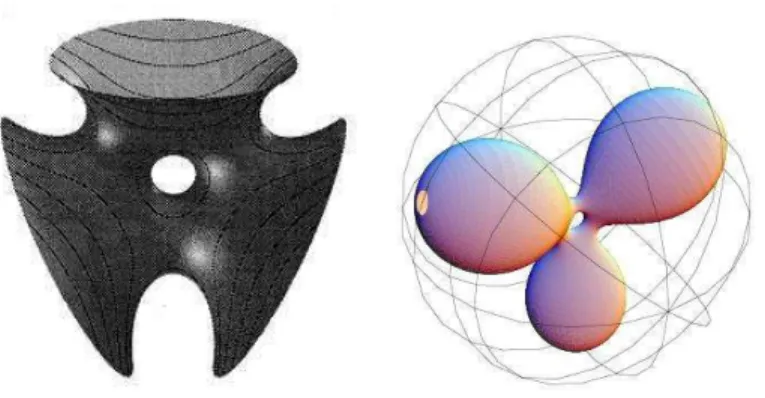
Figure 1: Half of a “dual” Enneper cousin in the Poincare model. The entire surface consists of the piece shown union its reflections across planes containing boundary curves. This surface has infinite total curvature, and therefore has infinite index.
we find that
F = cosh(z) sinh(z)−zcosh(z) sinh(z) cosh(z)−zsinh(z)
!
.
ThereforeG= dd(cosh((sinh(zz)))) = tanh(z).
Following the Weierstrass representation as formulated in [By], we have a constant mean curvature 1 surface given byFF¯t with secondary Gauss map g =z. (Note that, since we are usingF instead of F−1 to make the surface, the functiongis now the secondary Gauss
map, not the hyperbolic Gauss map.) In this case the secondary Gauss map is actually single valued, since the surface is simply connected. By Lemma 4.1, the second variation is determined by Σ =C∪ {∞} and g =z. For this Σ and g, the unconstrained index is Indu(M) = 1. This can be seen from Theorem 4.6 of [N1], or from Proposition 6.1 below.
It follows Ind(M) is either 0 or 1. But the Enneper cousin cannot be stable, since the horosphere is the only stable example ([Si]), hence Ind(M) = 1.
We can also consider Enneper cousins with winding order 2k+ 1 at the end, k∈N. In this case g becomes g = zk, and the other objects Σ = C∪ {∞} and Σ\ {pj} = C and f = 1 and c = 1 and z0 = 0 remain unchanged. Now, by [N1] or Proposition 6.1 below,
Indu(M) = 2k−1. Hence, by Lemma 5.3, the Enneper cousins with winding order 2k+ 1
have constrained index Ind(M) either 2k−1 or 2k−2.
Following the Weierstrass representation as formulated in Lemma 3.2 of this paper, we have a constant mean curvature 1 surface given byF−1F−1t, and this produces the “dual”
Enneper cousin that is described in [RUY]. The dual Enneper cousin has secondary Gauss map G= tanh(z) and hence has infinite total curvature. By [CS], it must therefore have infinite index. (See Figure 1.)
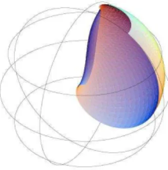
Catenoid cousins: A catenoid cousin has Σ\ {pj}=C\ {0}, and has secondary Gauss
mapG=zµ, whereµ6= 0,±1 is real. We can assume without loss of generality thatµ >0. The surface is embedded ifµ <1 and not embedded ifµ >1. (This is shown in [UY1]. It was originally shown in [By], but the parameterµis formulated differently in [By]. We use the same µ as in the [UY1] formulation. Figures of the catenoid cousins can be found in [UY1].)
proposition is proven in [N1] in the case that µis an integer. The proof when µ is not an integer is essentially the same. We include the proof here for the sake of completeness.
Proposition 6.1 Letµbe a positive real. The complete set of eigenvalues for the Laplacian
on the plane with the pull back metric from the sphere via the mapG=zµ is
λp,q= (p+
q
µ)(1 +p+ q
µ), p, q= 0,1,2, ... .
The multiplicity ofλp,q is 2 ifq >0 and is 1 ifq = 0.
Proof. We are considering the problem ¯△u=λu, where ¯△is the Laplacian obtained from
pulling back the standard metric on S2 via the map G = zµ. In polar coordinates this equation becomes
∂2u ∂r2 +
1 r ∂u ∂r + 1 r2
∂2u ∂θ2 =−λ
4µ2r2µ−2 (r2µ+ 1)2u .
For a real number α and a nonnegative integer i, we define (α)i to be (α)i = α(α+
1)...(α+i−1) ifi >0 and (α)i = 1 ifi= 0. We then define a real analytic hypergeometric
function F(a, b, c, x) where c is not a nonpositive integer. This function F(a, b, c, x) is defined for−1< x <1.
F(a, b, c, x) :=
∞
X
i=0
(a)i(b)i
i!(c)i
xi .
F(a, b, c, x) satisfies the hypergeometric differential equation
x(1−x)d
2y
dx2 + (c−(a+b+ 1)x)
dy
dx −aby= 0 .
For nonnegative integerspandq,F(p+ 2µq+ 1,−p,µq+ 1,12(1−t)) is a polynomial of degree p. We set
φp,q(t) = (1−t2)
q
2µF
p+ 2q
µ+ 1,−p, q µ+ 1,
1 2(1−t)
, −1< t <1
and
vp,q(r) =φp,q
r2µ−1 r2µ+ 1
!
, 0< r <∞ .
We can check that, for λ = (p+ µq)(1 +p+ µq), φp,q(t) satisfies the ordinary differential
equation
(1−t2)∂
2φ
∂t2 −2t
∂φ ∂t +
λ−(q µ)
2 1
1−t2
φ= 0 ,
and vp,q(r) satisfies the ordinary differential equation
∂2v
∂r2 +
1 r
∂v ∂r + λ
4µ2r2µ−2
(r2µ+ 1)2 −
q2
r2
!
v= 0 .
We can then check thatvp,q(r) cos(qθ) andvp,q(r) sin(qθ) are eigenfunctions of the Laplacian
Finally, we need to check that, for nonnegative p and q, the above eigenfunctions form a complete orthogonal system in theL2d¯s2 norm. This follows by elementary arguments. ✷
The following theorem follows immediately from Proposition 6.1 and Lemma 5.3, and from Silveira’s result that the horosphere is the only stable complete constant mean curva-ture 1 surface inH3 [Si].
Theorem 6.1 The index of any embedded catenoid cousin is exactly 1, and the index of
any nonembedded catenoid cousin is at least 2. Let[µ]be the greatest integer that is strictly less thanµ, then the index of the catenoid with value µis either 2[µ] + 1or 2[µ]. Thus, for any positive numberN there exists a catenoid cousin with index greater than N.
Remark. It is clear from the above proposition that when µ6∈ Z, the nullity (nullity :=
the dimension of the eigenspace corresponding to the eigenvalue 0) of the catenoid cousins is 1 (i.e. this is the case that p=1,q=0), and that whenµ∈Z, the nullity is 3 (p= 1, q= 0 orp= 0, q=µ). And the unconstrained index Indu(M) changes only asµ passes through
an integer, when two eigenvalues pass through 0. Furthermore, this illustrates another difference from the case of minimal surfaces in R3, where the nullity is always at least 3, since the set of translations make bounded normal Jacobi fields on a minimal surface ([N1],
[MR], [EK]). ✷
There are some other examples where we can compute the index explicitly, via the above proposition, which we will now describe.
Example 7.4 of [UY1] has a Weierstrass representation with G = zm, 3 ≤ m ∈ Z on
Σ\ {pj}=C\ {0}. It follows immediately from Proposition 6.1 and Lemma 5.3 that the
index Ind(M) of this example is either 2m−1 or 2m−2.
Another example is given in Theorem 6.2 of [UY1]. It has a Weierstrass representation with G = azℓ +b and Hopf differential Q = acℓz−2(dz)2 on Σ\ {pj} = C\ {0}, where
ℓ∈Z, ℓ6= 0 and a, b, c∈C,a= 0,6 c6= 0, and ℓ2+ 4acℓ=m2 for some positive integer m. In the case thatb= 0, we can simply rewritea1ℓz asz, and then Σ\ {pj}is unchanged
andGbecomesG=zℓ. Hence, whenb= 0, Ind(M) is either 2ℓ−1 or 2ℓ−2, by Proposition 6.1 and Lemma 5.3.
In the case that ℓ = 1, then we can make the transformation of the complex plane z → z−ba . Then Σ is still C∪ {∞}, and G becomes G = z1. Hence by Proposition 6.1
and Lemma 5.3, Ind(M) is either 0 or 1. By [Si] these surfaces cannot be stable, hence Ind(M) = 1. There are many different examples of this type with ℓ = 1: for example, ℓ= 1, a= 1, c = 2, m = 3, b = 0 or ℓ = 1, a = 34, c = 1, m= 2, b = 0, and infinitely many others.
Remark. This last example with ℓ = 1 illustrates another difference between minimal
surfaces in R3 and constant mean curvature surfaces in H3: While the only complete minimal surfaces in R3 with index 1 are the catenoid and Enneper’s surface ([FC], [Cho]), the embedded catenoid cousins and the Enneper cousins are not the only constant mean
curvature 1 surfaces inH3 with index 1. ✷
7
Lower bounds for Ind(
M
)
inH3. The results in section 5, particularly Lemma 5.3, are crucial to getting the method to work in our situation.
Let φ be a Killing vector field in H3 generated by either a hyperbolic rotation or a hyperbolic translation. For both a hyperbolic rotation and a hyperbolic translation there are two fixed points on the sphere at infinity, and we shall call these two points the points in the sphere at infinity fixed byφ. (For example, a Euclidean rotation about thex3-axis of
the upperhalf space model forH3 is a hyperbolic rotation, and a Euclidean dilation centered at the point x1 = x2 = x3 = 0 of the upperhalf space model is a hyperbolic translation.
Both of these isometries ofH3 fix the two points x1 =x2=x3 = 0 and x1 =x2=x3 =∞ in the sphere at infinity.)
Let M be a constant mean curvature 1 surface in H3 with finite total curvature. The Killing vector field φ can be decomposed into tangent and normal parts on M, that is, φ=φT +φ⊥, where φT ∈T(M) and φ⊥∈N(M), and N(M) is the normal vector bundle
of M. Choosing a unit normal N~ on M, it can be checked by a direct computation (see, for example, Lemma 1 of [Cho] or Proposition 2.12 of [BCE]) that the normal projection φ⊥ =u ~N of a Killing vector fieldφon M is a Jacobi field (i.e. △u+ 2Ku = 0).
Definition 7.1 LetH(M, φ) be the set of all points on M where φ⊥= 0. We callH(M, φ)
the horizonof M with respect to φ. Each component of M\H(M, φ) is called a visible set
of M. The number of visible sets of M\H(M, φ) is called the vision numberv(M, φ) of M
with respect to φ. The number of visible sets of M\H(M, φ) which are either bounded or whose closure intersects the sphere at infinity only at one or both of the points fixed by φis called the adjusted vision number ˜v(M, φ) of M with respect toφ.
Note that ˜v(M, φ)≤v(M, φ).
Theorem 7.1 LetM be a constant mean curvature 1 surface inH3 of finite total curvature
with regular ends. Then for any choice of φ,
Ind(M)≥v(M, φ)˜ −1
if ˜v(M, φ)6=v(M, φ), and
Ind(M)≥v(M, φ)˜ −2
if ˜v(M, φ) =v(M, φ).
Proof. First we show that on any visible set which is counted in ˜v(M, φ), u ~N is bounded.
(This is not true for the visible sets which are not counted in ˜v(M, φ).) For this, we need to use that we have regular finite total curvature ends. Note that the definition of a regular end is an end for which the hyperbolic Gauss map G extends holomorphically across pj
[UY1]. An end with finite total curvature is regular if and only if ordpj(Q)≥ −2 [By]. For
these types of ends, assuming that the end approaches the origin in the upper-half-space model, we have the following asymptotic behavior:
Re(zm),Im(zm), c|z|µ+m(1 +O(|z|min(1,2µ))) ,
that lim supz→0 f
|z|min(1,2µ) is bounded. (See the appendix for a proof of this asymptotic
behavior.) Note that the unit normal N~ is of the form
~
N = cx
µ+m
p
m2+c2(µ+m)2x2µ+O(1,2µ)(−c(µ+m)x µ(1 +
O(1,2µ)), xµO(1,2µ), m) over a pointz=x >0, x∈R.
We now consider three cases for the Killing vector field φ:
• Supposeφis made by an isometry which is either a hyperbolic rotation or a hyperbolic translation, and suppose that the originx1=x2=x3 = 0 is not one of the two points
in the sphere at infinity fixed by φ. In this case we may consider that φ ≈ (1,~0,0) near the origin. Thus, whenz=x >0, we have
hφ, ~NiH3 ≈ −
(µ+m)(1 +O(1,2µ))
xmpm2+c2(µ+m)2x2µ+O(1,2µ) ,
and this will diverge to ∞ as x → 0. Thus for a φ of this type, the normal Jacobi vector field φ⊥ = hφ, ~NiN~ is not bounded. (As a simple example, one can easily computehφ, ~Ni explicitly for a horosphere.)
• Supposeφis made by the isometry which is a dilation centered at the origin. In this caseφ=(x1, x~2, x3) at (x1, x2, x3). Thus, when z=x >0, we have
hφ, ~NiH3 = −
µ(1 +O(1,2µ))
p
m2+c2(µ+m)2x2µ+O(1,2µ) ≈
−µ m .
Thus, for a φof this type, the length hφ, ~NiH3 of the normal Jacobi vector field φ⊥
is bounded and continuous in a neighborhood of the end.
• Supposeφ is made by the isometry which is rotation about thex3-axis. In this case
φ=(−x2~, x1,0) at (x1, x2, x3). Thus, when z=x >0, we have
hφ, ~NiH3 =O(1,2µ) ,
and so the length hφ, ~NiH3 of the normal Jacobi vector field φ⊥ is bounded and
continuous in a neighborhood of the end.
Let u=hφ, ~NiH3 be the length of the normal variation vector field φ⊥. In the second
and third cases above,u is bounded and continuous at the end asymptotic to the origin in the upper half space model. Hence we can conclude from Harvey and Polking’s removable singularity theory ([HP], [P], [Cho]) thatu is a weak solution of the Jacobi operator △u+ 2Ku= 0 on Σ, except at the ends whereu is not bounded.
So on each visible set counted in ˜v(M, φ),uis bounded; and for each visible set counted in ˜v(M, φ), the nullity of the visible set with respect to the Dirichlet problem is at least 1.
The operator ¯Lon Σ has the following properties:
• L¯ satisfies theunique continuation property; that is, if two solutions uand vof ¯L= 0 are equal on any open set of Σ, then they are equal on all of Σ. This property holds on Σ simply because it holds on Σ\ {pj} (since any weak solution u of ¯Lu = 0 on
Σ\ {pj} is also a strong solution on Σ\ {pj}, by elliptic regularity), and because any