www.atmos-chem-phys.net/15/9917/2015/ doi:10.5194/acp-15-9917-2015
© Author(s) 2015. CC Attribution 3.0 License.
Meteor radar quasi 2-day wave observations over 10 years at Collm
(51.3
◦
N, 13.0
◦
E)
F. Lilienthal and Ch. Jacobi
Institute for Meteorology, University of Leipzig, Stephanstr. 3, 04103 Leipzig, Germany
Correspondence to:F. Lilienthal ([email protected])
Received: 3 February 2015 – Published in Atmos. Chem. Phys. Discuss.: 31 March 2015 Revised: 29 July 2015 – Accepted: 24 August 2015 – Published: 2 September 2015
Abstract. The quasi 2-day wave (QTDW) at 82–97 km
al-titude over Collm (51◦
N, 13◦
E) has been observed using a VHF meteor radar. The long-term mean amplitudes calcu-lated using data between September 2004 and August 2014 show a strong summer maximum and a much weaker winter maximum. In summer, the meridional amplitude is slightly larger than the zonal one with about 15 m s−1 at 91 km
height. Phase differences are slightly greater than 90◦
on an average. The periods of the summer QTDW vary between 43 and 52 h during strong bursts, while in winter the peri-ods tend to be more diffuse. On average, the summer QTDW is amplified after a maximum of zonal wind shear which is connected with the summer mesospheric jet and there is a possible correlation of the summer mean amplitudes with the background wind shear. QTDW amplitudes exhibit consider-able inter-annual variability; however, a relationship between the 11-year solar cycle and the QTDW is not found.
1 Introduction
The quasi 2-day wave (QTDW) is one of the most strik-ing dynamical features in the mesosphere and lower ther-mosphere. The QTDW was first reported by Muller (1972) using a meteor wind radar at Sheffield, UK. He found sig-nificant oscillations with periods of approximately 51 h from UK radar data. Even earlier, QTDWs were discovered over Mogadishu (Babadshanov et al., 1973) near the Equator. The QTDW at mid-latitudes is characterized by a clear maximum in summer, with one or several bursts of a few weeks each. At high latitudes the wave shows a different behavior com-pared to at mid-latitudes, e.g., with maxima during winter (Muller and Nelson, 1978; Nozawa et al., 2003). The QTDW
has been frequently observed by ground-based (e.g., Muller, 1972; Babadshanov et al., 1973; Plumb et al., 1987; Harris, 1994; Jacobi et al., 1997; Gurubaran et al., 2001; Chshy-olkova et al., 2005) and satellite instruments (Wu et al., 1996; Tunbridge et al., 2011). Additionally, several numerical stud-ies simulated possible excitation processes (Salby, 1981a, b; Plumb, 1983; Palo et al., 1999; Salby and Callaghan, 2001).
Regarding possible forcing mechanisms, Salby (1981a, b) suggested the QTDW to be a manifestation of a Rossby grav-ity normal mode in an isothermal windless atmosphere with wave number 3; however, this mechanism could not explain its burst-like behavior. Applying a one-dimensional stabil-ity analysis Plumb (1983) introduced baroclinic instabilstabil-ity as an excitation mechanism. Pfister (1985) supported this the-ory by using a two-dimensional quasi-geostrophic model and found a QTDW with wave numbers 2–4 and maxima at mid-dle and high latitudes. However, this result did not resemble all the characteristics of the observed wave. Hence, Salby and Callaghan (2001) combined both mechanisms in numer-ical experiments and found a QTDW excitation in the winter hemisphere by planetary wave activity. Crossing the Equa-tor to the summer hemisphere the QTDW is then enhanced by baroclinic instability connected with the easterly meso-spheric wind jet (Wu et al., 1996).
by Malinga and Ruohoniemi (2007); see also Pancheva et al. (2004) and Tunbridge et al. (2011). The dominating one has periods of approximately 48 h with wave numbers 2 and 3. The second group has much shorter periods of about 42–43 h. Different wave numbers such as 2, 3 and 4 are reported. The last group covers periods longer than 48 h and peaks at 52 h with wave numbers 2 and 3. In the SH these three groups could not be observed and periods are close to 48 h with wave number 3 (Wu et al., 1996; Walterscheid et al., 2015). Craig and Elford (1981) explored phase locking relative to the sun and suggested nonlinear interactions with diurnal tides. This is also supported by recent studies (e.g., Huang et al., 2013a; Moudden and Forbes, 2014; Walterscheid et al., 2015). A possible correlation of QTDW amplitudes with the 11-year solar cycle has been found by Jacobi et al. (1997), who ex-plained this finding by a stronger mesospheric wind shear during solar maximum.
In the following we present analyses of the QTDW from a meteor radar (MR) at Collm (51◦
N, 13◦
E) which was started in 2004. Earlier, the low-frequency (LF) spaced re-ceiver method was applied at Collm, from the late 1950s until 2007. This was based on the reflection of commercial LF ra-dio waves in the lower ionospheric E region. This led to reg-ular daily gaps due to increased absorption during daylight hours. These gaps are especially long in summer. The mea-surements had been used earlier to obtain a QTDW climatol-ogy over Collm (Jacobi et al., 1997). However, the limitations of the LF method may give rise to potential artifacts, namely uncertainties of the amplitude and possible effects on the ana-lyzed phases resulting from the data gaps. Therefore, here the MR winds are analyzed and can be used to evaluate the ear-lier results because meteor winds are observed continuously throughout the day. Possible MR data gaps owing to small meteor count rates especially at the uppermost and lower-most heights are shorter and more regularly distributed than the LF data gaps. Collm MR wind data from 2004 to 2013 have already been analyzed with respect to the climatology of a 2-day oscillation by Lilienthal and Jacobi (2014), but their analysis is based on a fixed period of 48 h. This may lead to different amplitudes and phases. In the present study, the ac-tual periods of the QTDW over Collm are calculated in order to improve the results of Lilienthal and Jacobi (2014). Com-pared with Jacobi et al. (1997), further information about the mid-latitude QTDW can be obtained with greater accuracy than the earlier LF measurements, in particular because the amplitude and phase uncertainties due to daytime data gaps of LF measurements will be avoided. Background shear ob-tained from the prevailing winds observed by the radar is used as a proxy for baroclinic instability.
2 Measurements and data analysis
A commercial VHF MR, distributed under the brand name SKiYMET (All-Sky Interferometric Meteor Radar;
Hock-ing et al., 2001) is operated at Collm Observatory (51◦N,
13◦E) since late summer 2004 to measure mesopause region
winds, replacing the earlier LF drift measurements (e.g., Ja-cobi et al., 1997). The MR operates at 36.2 MHz and has a pulse repetition frequency of 2144 Hz which is effectively reduced to 536 Hz due to a 4-point coherent integration. The peak power is 6 kW. The transmitting antenna is a 3-element Yagi with a sampling resolution of 1.87 ms and an angular and range resolution of about 2◦
and 2 km, respectively. The receiving interferometer consists of five 2-element Yagi an-tennas arranged as an asymmetric cross. This allows calculat-ing the azimuth and elevation angle from phase comparisons of the individual receiver antenna pairs. Together with range measurements, the meteor trail position is detected. The radar uses the Doppler shift of the reflected VHF radio wave from ionized meteor trails in order to measure the radial velocity along the line of sight of the radio wave. The radar and data collection procedure is described by Hocking et al. (2001).
The meteor trail reflection heights vary between 75 and 110 km with a maximum around 90 km (e.g., Stober et al., 2008). To analyze the wind field, the received meteors and corresponding radial winds are binned in six height gates centered at 82 km (80.5–83.5 km), 85 km (83.5–86.5 km), 88 km (86.5–89.5 km), 91 km (89.5–92.5 km), 94 km (92.5– 96.0 km) and 98 km (96.0–100.5 km). With regard to the up-permost height gate, Jacobi (2012) showed that, owing to the vertical distribution of meteor count rates, nominal and mean heights are not necessarily the same and that the uppermost gate has a nominal height of 98 km which refers to a mean height of about 97 km. The radar measurements deliver half-hourly mean horizontal wind values that are calculated by a least squares fit of the horizontal half-hourly wind compo-nents to the individual radial wind under the assumption that vertical winds are small (Hocking et al., 2001). An outlier re-jection is added. The climatology of background winds and tides as measured by the Collm radar is presented in Jacobi (2012).
pe-8 16 24 32 40 48 56 64 0
5 10 15 20 25 30 35
a
m
p
lit
u
d
e
[
m
s
-1 ]
period [h]
25/07/2010
Figure 1.Lomb–Scargle periodogram of the meridional wind for a
time interval of 11 days centered on 25 July 2010 (91 km altitude). The QTDW period for this day is set to the one with the maximum amplitude between 40 and 60 h, illustrated by the vertical dotted line.
riod difference is generally small and <2 h in about 75 % of all cases with large amplitudes. Hence, the underestima-tion of zonal amplitudes is small and, as will be described in Sect. 3.1, the zonal amplitude is smaller than the meridional one even when using QTDW periods that are based on a odogram analysis for the zonal component. An example peri-odogram analysis for the meridional component is shown in Fig. 1, using data of a time interval centered on 25 July 2010. In this case, the amplitude maximum between 40 and 60 h is found at a period slightly larger than 40 h, which represents the QTDW period for this date.
To obtain amplitudes and phases of the QTDW a least-squares fit has been applied to the zonal and meridional hori-zontal half-hourly winds, which includes the prevailing wind, tidal oscillations of 24, 12 and 8 h, and the individual period of the QTDW as obtained from the periodogram analysis of the meridional wind. Each individual fit is again based on 11 days of half-hourly mean winds and the results are attributed to the center of this data window. Note that if shorter data windows were used, the resulting amplitudes would be re-duced. In particular, this is the case if there are 2-day bursts within the 11-day window which are not coherent. This has been discussed by Jacobi et al. (1997) who used both 11-and 5-day windows for their analysis. Choosing windows that are too small would thus include more irregular fluctua-tions, while the chosen 11-day window usually covers several cycles within a QTDW burst. For the example presented in Fig. 1, the resulting amplitude of the QTDW is 27.6 m s−1
at a period of 40.5 h. After analyzing the QTDW parameters in an 11-day window, the window was shifted by 1 day. The least-squares fit was performed for both the zonal and the meridional wind component, and for each height gate sepa-rately. The following results are based on these data.
0 30 60 90 120 150 180 210 240 270 300 330 360
0 10 20 30 40 50
averages 09/2004-08/2014: total amplitude meridional amplitude zonal amplitude 45-day adjacent average of total amplitude
single year total amplitudes
w
in
d
s
h
e
a
r
[m
s
-1k
m
-1]
a
m
p
lit
u
d
e
[
m
s
-1]
day of year
-8 -6 -4 -2 0 2 4 6
wind shear
30 60 90 120 150 180 210 240 270 300 330 360 82
85 88 91 94 97
h
e
ig
h
t
[k
m
]
day of year
6 m/s 10 m/s 14 m/s 18 m/s 22 m/s amplitude
Figure 2.Upper panel: total annual amplitudes between
Septem-ber 2004 and August 2014 (light gray). Average values of the years 2004–2014 in black for total (straight), meridional (dashed) and zonal (dotted) components. The 45-day adjacent average for the to-tal annual amplitude is in red. The blue curve denotes the vertical shear of zonal wind including standard error. Data refer to an alti-tude of 91 km. Lower panel: contour plot of the 10-year mean am-plitudes over height in an annual cycle. The horizontal lines (black) mark the six height gates. Data are interpolated in between.
3 Results
The upper and lower panels of Fig. 2 present the mean sea-sonal cycle of QTDW amplitudes. Here, we also present the total amplitudes as a combination of zonal and meridional components. The upper panel of Fig. 2 refers to an altitude of 91 km (gate 4). It shows the total amplitudes of each year in light gray, starting in September 2004 and ending in Au-gust 2014. The black lines show the 10-year average for to-tal (straight), meridional (dashed) and zonal (dotted) ampli-tudes and the red line shows 45-day adjacent averages of the 10-year mean total amplitude. As previously reported in the literature, we find a strong summer and a weaker win-ter maximum. The first increase of the summer burst starts during May, where the year 2006 shows a strikingly strong burst. Maximum amplitudes are usually reached at the end of July and beginning of August, where the long-term average amplitudes (red curve) exceed 15 m s−1. The maxima
dur-ing individual bursts (gray curves) can be even larger and in some years they reach up to 40 m s−1. The winter QTDW
ap-pears much weaker with average amplitudes between 5 and 10 m s−1.
compo-Figure 3.Periodograms of the meridional amplitude for the years 2004–2014 at 91 km altitude. Each day represents the center of an 11-day analysis of horizontal wind data. The white line follows the period of maximum amplitude between 40 and 60 h if amplitudes are larger than 6 m s−1.
nents at 94 and 88 km, is added as a blue line. On a long-time average, the QTDW amplitudes start to increase when the shear reaches its maximum. In Sect. 3.1, we show that wind shear, taken here as a proxy for baroclinic instability, may act as a source of the QTDW. However, this relation is not ob-served in winter where the QTDW is assumed to appear due to instabilities of the polar night jet (e.g., Venne and Stanford, 1982; Hartmann, 1983; Sandford et al., 2008; Baumgaertner et al., 2008).
Generally, the meridional amplitude in Fig. 2 is larger than the zonal one. One may argue that this is due to the fact that we define the period of the QTDW as the period of
maxi-mum meridional amplitude (see Fig. 1). This ensures strong meridional amplitudes at the chosen period but may result in smaller zonal amplitudes if the maximum zonal value is found at another period. To prove that the larger meridional component is not attributed to the analysis method we per-formed the same analysis but determined the period of the QTDW from the zonal component (not shown here). As a re-sult, the meridional QTDW amplitude is still larger than the zonal one.
42 44 46 48 50 52 54 56 58 0
20 40 60 80 100 120
all amplitudes vtot>10ms-1
vtot>15ms -1
c
o
u
n
ts
period [h]
May-Aug 2005-2014 altitude: 91km
Figure 4.Distribution of QTDW periods in summer (May–Aug) for
the years 2005–2014. Black: amplitudes larger 15 m s−1only. Gray: amplitudes between 10 and 15 m s−1. White: amplitudes smaller
than 10 m s−1.
The seasonal cycle is similar at different height gates except for the uppermost one. The summer amplitudes maximize at about 88 km height which is close to the value reported by Chshyolkova et al. (2005). The winter maximum is strongest at higher altitudes in late winter where 10 m s−1can be
ex-ceeded, so that at the upper height gate, the amplitude differ-ence between summer and winter decreases.
The distribution of meridional amplitudes during the years 2004–2014 as obtained from the Lomb–Scargle peri-odograms is shown in Fig. 3. As in Fig. 2, they refer to an altitude of 91 km. The white line denotes the period of max-imum amplitude between 40 and 60 h. Note that this curve determines the period that is taken as the real QTDW pe-riod for further analyses. Having a look at the summer sea-son it is apparent that in certain years the QTDW appears in one single burst (such as 2007, 2010 or 2012) with typi-cal seasonal maxima at the end of July or beginning of Au-gust. In other years, QTDW activity is split into two or more bursts (e.g., 2005, 2006, 2009). The largest amplitudes are usually found between June and August; however, in some years (e.g., 2006, 2009, 2014) significant amplitudes are also observed in May. The running spectrum for 2006 is a typical example for a strong summer QTDW with two main bursts where the periods vary between more or less 40 and 52 h. At the onset of the summer wave in May and when it vanishes in August, the periods are longer than during the event. This feature from long periods to shorter ones and back to long ones is also seen in other years such as 2007 and 2012. In 2005 and 2009 the period is also largest at the onset of the wave burst and lowest at the maximum of the wave, but it is more variable in between.
In each winter from 2005 to 2014 slightly increased am-plitudes of the QTDW can be seen. The 10-year mean winter maximum is small and the amplitudes are, on average, only about 2 times as large as during the September minimum, which is comparable to earlier observations (e.g., Muller and Nelson, 1978). The winter oscillations are irregular: they are particularly large in January 2006, 2012 and 2013. In some cases the enhancement already starts at the end of the previ-ous year, e.g., large amplitudes in December 2011 continue in January 2012. Several studies (e.g., Gu et al., 2013; Lima et al., 2012; McCormack et al., 2009) suggest a possible rela-tion between QTDW amplitudes and the strong major sudden stratospheric warming in January 2006. The 2012 and 2013 maxima are also found during winters of major stratospheric warmings: however, during the 2009 stratospheric warming no QTDW enhancement is seen in the measurements. In some years (e.g., 2009, 2011, 2012) amplitudes also maxi-mize in November or December. Periods are very short in January with 44 h or less and they increase until February where they often reach 52 h or more.
In the following we concentrate on the more intense sum-mer QTDW, referring to the months of May–August. In or-der to investigate the distribution of periods with respect to the amplitudes, Fig. 4 shows histograms of periods for dif-ferent magnitudes of the amplitude where boundary periods (≤41 h or>59 h) are omitted. Dark bars denote only larger amplitudes while white bars include days of all amplitudes. The histogram refers to an altitude of 91 km during summer (May–August). As a result, intervals with large QTDW am-plitudes tend to exhibit shorter periods. The median for large amplitudes (black columns) is 47.9 h but the median for all amplitudes including small ones (white) is 49.3 h. For am-plitudes larger than 15 m s−1(black columns), the lower and
upper quartiles are 45.8 and 52.7 h, respectively. For larger periods, smaller amplitudes dominate. Furthermore, we find a clear maximum at 47–48 h and two secondary maxima at 42–43 h and 50–51 h. The latter two maxima are not statis-tically significant but, together with the primary maximum, they correspond to the three maxima presented by Malinga and Ruohoniemi (2007).
In the following we show summer QTDW data for ampli-tudes of at least 15 m s−1. Figure 5 shows the relative
am-plitude differences1v(see Jacobi, 2012) between zonal and meridional QTDW amplitudes at 91 km altitude given by
1v=2vz−vm
vz+vm
·100 %, (1)
where the index z refers to the zonal and the index mto the meridional component of the QTDW. Hence, positive (negative)1v values denote larger zonal (meridional) am-plitudes and the value denotes the percentage of amplitude differences from the mean amplitude. The mean and median of summer relative amplitude differences amount to−46.8 and−39.0 %, respectively. The 5 and 95 % percentiles are
-150 -100 -50 0 50 100 0
5 10 15 20 25 30 35 40
relative amplitude difference [%] Jan-Dec
May-Aug
c
o
u
n
ts
v
tot(91km) > 15ms
-1
Figure 5.Histogram of the 91 km (gate 4) relative amplitude
differ-ences1vof zonal and meridional components for amplitudes larger than 15 m s−1. Black bars: summer (May–August) data, 460 days
considered. White bars: rest of the year (January–April, September– December) data, 17 days considered. Positive values denote larger zonal than meridional amplitudes.
meridional component tends to be larger than the zonal one. Note that the meridional amplitude also tends to be slightly larger due to the fact that the periods of the QTDW were cho-sen from the maximum meridional amplitude. However, this effect is small. If we calculate the relative amplitude differ-ences using the periods at maximum zonal amplitude we ob-tain P5= −75.5 % and P95=17.1 %, which qualitatively leads to the same conclusion that the meridional amplitude is larger.
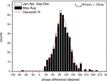
The phase differences between zonal and meridional QTDW components at 91 km altitude are shown in Fig. 6. The histogram includes the results for amplitudes larger than 15 m s−1in black and white for summer (May–August) and
the rest of the year, respectively. The small number of the latter shows that large amplitudes do mainly appear in sum-mer. A Gaussian fit was applied to the summer histogram. As a typical feature of that distribution, mean (102.2◦
), median (101.1◦
) and mode (102.4◦
) are all of similar value. These values are only slightly larger than 90◦
and hence the zonal and meridional components are nearly in quadrature. Other height gates have Gaussian modes that are up to 10◦larger
compared to the 91 km altitude.
Figure 7 (left panel) shows the means and standard devi-ations of the phase difference at all six height gates for am-plitudes larger than 15 m s−1. The standard deviation of the
uppermost gate is almost twice as large as those of the lower gates. Considering the lower gates, the means are compara-ble to the one at 91 km, slightly higher than 90◦
. However, the standard deviation of about 30◦
is large. The right panel of Fig. 7 shows the profile of the mean QTDW zonal and meridional amplitudes as well as their differences. At 82 km
-120 -90 -60 -30 0 30 60 90 120 150 180 210 240 270 300 0
10 20 30 40 50 60
70 Jan-Apr, Sep-Dec
May-Aug Gaussian fit
phase difference [degree]
c
o
u
n
ts
v
tot,48(91km) > 15ms -1
Figure 6. Histogram of the 91 km (gate 4) phase differences
of zonal and meridional components for amplitudes larger than 15 m s−1. Black bars: summer (May–August) data, 460 days
con-sidered. White bars: rest of the year (January–April, September– December) data, 17 days considered.
the meridional amplitude is only slightly larger than the zonal one. For greater altitudes, the difference is increasing up to a height of 91 km and almost constant above.
Vertical wavelengthsλz were calculated for each 11-day
interval when the amplitudes at the 91 km altitude were larger than 15 m s−1by
λz=
P
dT /dz, (2)
whereP is the period and dT /dzis the vertical gradient of the phaseT. For this analysis, the same period has to be used for each height gate to obtain consistent phases. Therefore, for wavelength calculation, we repeated the QTDW analysis for each height gate with the period found for 91 km. The ver-tical phase gradients were calculated by applying linear fits of phase over height. The histogram in Fig. 8 shows all wave-lengths smaller than 400 km. Indeed, we obtain a few very large (“infinite”) wavelengths that are not presented when the phase does not significantly change with altitude, i.e., when the wave does not propagate vertically. This is true in about 12 % of all cases considered. For the values smaller than 400 km, a lognormal probability density function is ap-plied. This fit is accepted by several statistical hypothesis tests such as a Kolmogorov–Smirnov, Anderson–Darling and a chi-squared test. The mode of the fitted lognormal function is 77 km whereas the median and mean of the data set for
<400 km are much larger with 106 and 127 km, respectively.
3.1 Connection with background wind shear
82 85 88 91 94 97
30 60 90 120 150 180 210
h
e
ig
h
t
[k
m
]
vtot > 15ms -1
phase difference [degree] 2 5 8 1 4 7
-14 -12 -10 -8 -6 -4 -2 0 2 4 6 810 12 14 16 18 20 22 24 vtot > 15ms
-1
amplitude [ms-1
] zonal meridional difference (z-m)
Figure 7.Left panel: mean phase difference (black) between zonal
and meridional components for 2004–2014 and their standard devi-ations. Right panel: zonal (red) and meridional (green) mean ampli-tudes for 2004–2014 and their standard deviations. Amplitude dif-ference with standard deviation in blue. For both panels only dates with total amplitude>15 m s−1are used.
northward gradient of quasi-geostrophic potential vorticity
qy must change sign somewhere in the flow domain to
en-able instability (Charney and Stern, 1962). This condition is given in the summer mesospheric jet in an altitude of about 70 km. Here, the vertical zonal wind profile has a minimum or, in other words, the easterly winds to reach a maximum. In order to investigate possible baroclinic instability by analyz-ing MR measurements from higher altitudes, a proxy needs to be determined because the wind maximum is outside the measurement range. We analyze the vertical wind shear of the zonal wind above the jet as a measure of its strength and hence for baroclinic instability.
We apply superposed epoch analyses in two ways. First, the key events are defined from the time series of the am-plitude. Therefore, the time series is filtered using a Lanc-zos low-pass filter with 30 weights and a cutoff period of 20 days. When the low-pass filtered amplitudes show a maxi-mum of at least 10 m s−1, a time window of the original time
series from 20 days before the event until 10 days after the event is considered. Second, the key events are defined from the time series of the wind shear which was again low-pass filtered with a cutoff period of 20 days. Maxima of at least 3 m s−1km−1are considered and the time window from−10
to+20 days is used. For each approach, separately, the time windows are averaged over all key events in both variables, amplitude and wind shear. Note that the maximum of the key variable is not necessarily placed at day 0 since the maxi-mum of the low-pass filtered values was set to day 0 but not the real time series. The results for an altitude of 85 km are shown in Fig. 9. If the QTDW was amplified by baroclinic instability, a maximum of the amplitudes would be expected to appear shortly after a maximum of wind shear as reported by Pendlebury (2012) or Ern et al. (2013). In Fig. 9, both methods of the epoch analysis show that the amplitude max-imizes about 10–15 days after a maximum of wind shear.
0 50 100 150 200 250 300 350 400
0 5 10 15 20 25 30 35 40 45 50 55 60
05/2005-08/2014 vtot(91km) > 15ms-1 40h < period < 60h
wavelength [km] May-Aug
c
o
u
n
ts
Lognormal PDF
Figure 8.Histogram of daily vertical wavelengths during summer
(May–August) for the time period from 2005 to 2014 (red bars) where only dates with total amplitude>15 m s−1are used.
Wave-lengths longer than 400 km are not shown (this refers to 56 days out of 460). A fitted lognormal probability density function in black.
These results are consistent with the conclusion of Plumb et al. (1987): the QTDW is propagating eastward, opposite to the wind direction in the jet. With increasing amplitude, it tends to act against its origin (Pendlebury, 2012; Ern et al., 2013) and diminishes the wind shear. When the wind shear is too weak for amplification the amplitude decreases again. However, considering the large error bars in our data we can only speak about tendencies. The effect is not clear enough to prove the hypothesis of baroclinic instability as a forcing mechanism. Furthermore, the results shown here at 85 km al-titude become less significant for higher alal-titudes.
3.2 Inter-annual variability
A correlation of QTDW amplitudes to the 11-year solar cycle was found in low frequency measurements by Jacobi et al. (1997) and recently by Huang et al. (2013b) using satellite measurements. Both report larger amplitudes during solar maximum. Due to the deep solar minimum in 2008 and 2009 an analysis of the inter-annual variability of the QTDW is of special interest. Figure 10 presents the F10.7 solar radio flux (black) and vertical zonal wind shear at 85 km (pink) in the upper part. The lower part shows the total amplitudes at the four height gates between the 85 and 94 km altitudes. These parameters are given for summer (upper panel) and winter (lower panel). The seasonal mean data presented in Fig. 10 are shown each as a 4-month average from May to August and from November to February while the year of the winter refers to the one of the respective January.
correla--20 -15 -10 -5 0 5 10 6 7 8 9 10 11 12 13 14 15 16 17 18 19 amplitude time [days] s h e a r [m s -1k m -1] a m p lit u d e [ m s -1] 4,0 4,5 5,0 5,5 amplitude > 10ms-1 altitude: 85km shear 10-day AAv of wind shear
-10 -5 0 5 10 15 20
6,5 7,0 7,5 8,0 8,5 9,0 9,5 10,0 10,5 11,0 11,5 12,0 s h e a r [m s -1k m -1] a m p lit u d e [ m s -1 ] time [days]
amplitude 10-day AAv of amplitude
3,5 4,0 4,5 5,0 5,5
shear shear > 3ms
-1 km-1 altitude: 85km
Figure 9.Superposed epoch analysis of vertical wind shear of the
zonal prevailing wind in blue and QTDW total amplitudes in red at 85 km altitude, including standard error. The 10-day adjacent averages of the amplitude are in dark red and wind shear in dark blue. Upper panel: maxima in wind shear>3 m s−1km−1are
con-sidered as key events. Lower panel: maxima in QTDW amplitude
>10 m s−1are considered as key events.
tion with the solar cycle is weak and insignificant. However, the correlation of the seasonal mean total amplitudes with the wind shear at 85 km altitude is stronger with correlation coefficients fromR=0.4 to 0.7. The zonal amplitude has a slightly larger correlation coefficient for all height gates; the meridional one is slightly smaller. However, either of them only differs by about 0.1. Jacobi and Ern (2013) report that gravity wave interactions reach particularly high altitudes in 2008 and hence further increase the shear which is also vis-ible in Fig. 10. However, this does not seem to affect the QTDW in summer.
In winter, amplitudes at different altitudes are not always as homogeneous as in summer. However, there is a clear peak in all altitudes during winter 2005/2006 when a major strato-spheric warming was observed. This is in good agreement with the general view that enhanced planetary wave activ-ity can cause stratospheric warmings. The correlation
be-2005 2006 2007 2008 2009 2010 2011 2012 2013 2014 4 8 12 16 20 24 year 82km 4 8 12 16 20 24 a m p lit u d e [ m s -1 ] 85km 4 8 12 16 20 24 a m p lit u d e [ m s -1] 88km 4 8 12 16 20 24 91km 60 80 100 120 140 160 F 1 0 .7 [ s .f .u .] summer (May-Aug) 85km 3 4 5 6 s h e a r [m s -1k m -1]
2005 2006 2007 2008 2009 2010 2011 2012 2013 2014 4 6 8 10 year 82km 4 6 8 10 a m p lit u d e [ m s -1 ] 85km 4 6 8 10 12 a m p lit u d e [ m s -1] 88km 4 6 8 10 12 91km 50 100 150 200 F 1 0 .7 [ s .f .u .] winter (Nov-Feb) -2 -1 0 1 s h e a r [m s -1k m -1] 85km
Figure 10.Seasonal mean QTDW total amplitudes for summer
(May–August, upper panel) and winter (November–February, lower panel, the year refers to the one of the respective January) for dif-ferent altitudes in orange, green, blue and red. Error bars denote the standard error given by the standard deviation of the 11-day anal-yses during one season divided by the square root of independent samples (11 per season). Seasonal mean F10.7 solar radio fluxes and their standard deviations given in solar flux units (sfu) where 1 sfu=10−22Wm−2Hz−1(black) and zonal wind shear of the
pre-vailing wind at 85 km and their standard errors (pink) are added.
tween QTDW winter amplitudes and solar radio flux in the lower height gates is slightly higher than in summer but still not significant. Correlation coefficients vary between−0.4 and+0.4, where zonal amplitudes tend to have negative val-ues and meridional ones tend to have positive valval-ues. The opposite holds for the correlation with wind shear. Here, meridional amplitudes tend to be negatively correlated (up to
How-ever, for different altitudes, the values differ significantly and most correlations turn out to be insignificant. This is in ac-cordance with the general view that the winter QTDW is a result of instability of the polar night jet and that the QTDW is originating from the lower atmosphere instead of being de-termined by the mesospheric circulation.
As presented in the periodograms in Fig. 3, the appearance of the QTDW is not uniform in each year. This is why one might expect a seasonal mean not necessarily to be repre-sentative enough to describe the QTDW. Thus, we also com-pare different ways to describe seasonal mean QTDW activ-ity during a season such as (1) the maximum total amplitude during a season, (2) the mean of the squared total amplitudes during a season as an estimate for energy, and (3) the mean of amplitudes minus a threshold value of 6 m s−1, while
neg-ative values are set to zero. This latter value is taken from the “noise floor” visible in Fig. 2 during the equinoxes.
As a result, the estimates (2) and (3) behave very similar to the seasonal mean values concerning magnitudes and sign of the correlation coefficients for correlations with solar radio flux and vertical shear of the zonal wind.
Using the maximum as an estimate, the correlation with solar radio flux in summer turns out to be slightly positive for most altitudes with R≈0.2 in the lower height gates. However, this is still no clear correlation and thus the results more or less correspond with those obtained for other esti-mates. The same holds for summer, where positive values for zonal and negative values for meridional amplitudes domi-nate. The correlation between wind shear and seasonal max-ima is mostly weaker than that obtained for seasonal means by about 0.2.
To conclude, differences obtained with the four meth-ods are not very large. Thus, the obtained relation between QTDW amplitudes and wind shear is robust and independent from the chosen method.
4 Discussion and conclusion
The QTDW is analyzed from Collm VHF meteor radar data. The considered time series begins after the installation of the radar in 2004 when it replaced earlier LF measurements (Ja-cobi et al., 1997) and continues until 2014.
On a 10-year average, the QTDW has amplitudes of about 15 m s−1in summer when analyzed on an 11-day basis, and
single bursts can reach values of 40 m s−1. These values are
comparable to those obtained by Guharay et al. (2013), but they presented MR measurements at low latitudes. In winter, a secondary maximum with amplitudes of 5–10 m s−1is
ob-served. These observations combined with the fact that e.g., Muller and Nelson (1978) and Nozawa et al. (2003) report a strong winter QTDW at high latitudes indicate that the in-fluence of the winter QTDW becomes stronger with increas-ing latitude. The periods of the QTDW tend to be longer in winter than in summer. Some years show a typical
signa-ture of periods during summer bursts that change in length from long to short and back to long while shorter periods are generally associated with larger amplitudes. Similar fea-tures were observed by Jacobi et al. (1997) and by long-term measurements at Saskatoon, Canada, by Chshyolkova et al. (2005). Tsuda et al. (1988) and Williams and Avery (1992), however, observed shortening periods during the respective bursts, while Pendlebury (2012) found continuously increas-ing periods durincreas-ing a burst.
Phase differences between the zonal and meridional com-ponent turn out to be slightly larger than 90◦
, which indicates that the wave is nearly but not exactly circularly polarized. This value is a bit larger than the one reported by Jacobi et al. (1997). The zonal and meridional amplitudes are of compa-rable size at 82 km altitude but they change with height in a way that the meridional ones tend to be larger by about 50 %. This coincides with the results of, e.g., Pancheva et al. (2004) and Gurubaran et al. (2001) but it could not be seen in the earlier LF measurements (Jacobi et al., 1997, 2001).
Vertical wavelengths were calculated from the vertical phase gradients. The mode of a fitted lognormal distribution is 77 km, while the median wavelength is 106 km. These val-ues are comparable to those obtained by Thayaparan et al. (1997). Smaller values below 80 km are reported, e.g., by Gurubaran et al. (2001), Guharay et al. (2013) or Huang et al. (2013b). Even larger values are found by Craig and Elford (1981) and Harris (1994) but these were obtained in the Southern Hemisphere. What all studies have in common is the fact that very large, almost “infinite” values were oc-casionally obtained, which is also the case over Collm. This indicates that the wave does not propagate vertically in these cases.
Furthermore, we find a connection between vertical zonal wind shear and QTDW amplitudes by applying superposed epoch analyses. They show a maximum of amplitudes about 10 days after a maximum of zonal wind shear at 85 km alti-tude. Also, a maximum of zonal wind shear is found about 10–15 days before the amplitude maximizes at 85 km. In the long-term mean annual cycle, zonal wind shear reaches a maximum when the QTDW starts to amplify. Also, in an inter-annual view, the correlation between zonal wind shear and amplitudes of the QTDW is high in summer but not in winter where the QTDW is assumed to be amplified by insta-bility of the polar night jet (e.g., Venne and Stanford, 1982; Hartmann, 1983; Sandford et al., 2008; Baumgaertner et al., 2008). Since shear is taken here as a proxy for baroclinic in-stability we conclude that the QTDW over Collm is at least to a certain degree forced by instability of the summer meso-spheric jet, as reported by Ern et al. (2013), using satellite measurements too. Also, Huang et al. (2013b) observed in-creasing QTDW amplitudes above regions of negative quasi-geostrophic potential vorticity.
correlation is not that clear. This can be explained by consid-ering the results of Jacobi et al. (2011). They found a positive correlation of zonal wind shear and solar cycle except dur-ing solar minimum when correlation turns out to be negative. This may also hold for the QTDW due to the possible am-plification by baroclinic instability. As the strong solar min-imum in 2009 is centered in the analyzed time series, longer observations are necessary to draw further conclusions.
Acknowledgements. We acknowledge the support from the German Research Foundation (DFG) and Universität Leipzig within the program of open-access publishing. F10.7 solar radio flux data have been provided by NGDC through FTP access at http://ftp.ngdc.noaa.gov/STP/SOLAR_DATA/.
Edited by: W. Ward
References
Babadshanov, P. B., Kalchenko, B. V., Kashcheyev, B. L., and Fe-dynsky, V. V.: Winds in the equatorial lower thermosphere, P. Acad. Sci. USSR, 208, 1334–1337, 1973.
Baumgaertner, A. J., McDonald, A. J., Hibbins, R. E., Fritts, D. C., Murphy, D. J., and Vincent, R. A.: Short-period planetary waves in the Antarctic middle atmosphere, J. Atmos. Solar-Terr. Phys., 70, 1336–1350, doi:10.1016/j.jastp.2008.04.007, 2008. Charney, J. G. and Stern, M. E.: On the Stability of Internal
Baro-clinic Jets in a Rotating Atmosphere, J. Atmos. Sci., 19, 159–172, doi:10.1175/1520-0469(1962)019, 1962.
Chshyolkova, T., Manson, A., and Meek, C.: Climatology of the quasi two-day wave over Saskatoon (52◦N, 107◦W): 14 Years of MF radar observations, Adv. Space Res., 35, 2011–2016, doi:10.1016/j.asr.2005.03.040, 2005.
Craig, R. L. and Elford, W. G.: Observations of the quasi 2day wave near 90 km altitude at Adelaide (35◦S), J. Atmos. Terr. Phys., 43, 1051–1056, doi:10.1029/1999JA900030, 1981.
Ern, M., Preusse, P., Kalisch, S., Kaufmann, M., and Riese, M.: Role of gravity waves in the forcing of quasi two-day waves in the mesosphere: An observational study, J. Geophys. Res., 118, 3467–3485, doi:10.1029/2012JD018208, 2013.
Gu, S.-Y., Dou, X., Wang, N.-N., Riggin, D. M., and Fritts, D. C.: Long-term observations of the quasi two-day wave by Hawaii MF radar, J. Geophys. Res. Space Phys., 118, 7886–7894, doi:10.1002/2013JA018858, 2013.
Guharay, A., Batista, P. P., Clemesha, B. R., and Schuch, N. J.: Study of the quasi-two-day wave during summer over Santa Maria, Brazil using meteor radar observations, J. Atmos. Solar-Terr. Phys., 92, 83–93, doi:10.1016/j.jastp.2012.10.005, 2013. Gurubaran, S., Sridharan, S., Ramkumar, T. K., and Rajaram, R.:
The mesospheric quasi-2-day wave over Tirunelveli (8.7◦N), J. Atmos. Solar-Terr. Phys., 63, 975–985, doi:10.1016/S1364-6826(01)00016-5, 2001.
Harris, T. J.: A long-term study of the quasi-two-day wave in the middle atmosphere, J. Atmos. Terr. Phys., 56, 569–579, doi:10.1016/0021-9169(94)90098-1, 1994.
Hartmann, D. L.: Barotropic Instability of the Polar Night Jet Stream, J. Atmos. Sci., 40, 817–835, doi:10.1175/1520-0469(1983)040<0817:BIOTPN>2.0.CO;2, 1983.
Hocking, W., Fuller, B., and Vandepeer, B.: Real-time deter-mination of meteor-related parameters utilizing modern dig-ital technology, J. Atmos. Solar-Terr. Phys., 63, 155–169, doi:10.1016/S1364-6826(00)00138-3, 2001.
Huang, K. M., Liu, A., Lu, X., Li, Z., Gan, Q., Gong, Y., Huang, C. M., Yi, F., and Zhang, S. D.: Nonlinear coupling between quasi 2 day wave and tides based on meteor radar obser-vations at Maui, 118, J. Geophys. Res.-Atmos., 3467–3485, doi:10.1002/jgrd.50872, 2013a.
Huang, Y. Y., Zhang, S. D., Yi, F., Huang, C. M., Huang, K. M., Gan, Q., and Gong, Y.: Global climatological variability of quasi-two-day waves revealed by TIMED/SABER observa-tions, Ann. Geophys., 31, 1061–1075, doi:10.5194/angeo-31-1061-2013, 2013b.
Jacobi, C.: 6 year mean prevailing winds and tides measured by VHF meteor radar over Collm(51.3◦N, 13.0◦E), J. Atmos. Solar-Terr. Phys., 78–79, 8–18, doi:10.1016/j.jastp.2011.04.010, 2012.
Jacobi, C. and Ern, M.: Gravity waves and vertical shear of zonal wind in the summer mesosphere-lower thermosphere, Rep. Inst. Meteorol. Univ. Leipzig, 51, 11–24, 2013.
Jacobi, C., Schminder, R., and Kürschner, D.: The quasi 2-day wave as seen from D1 LF wind measurements over Central Europe (52◦N, 15◦E) at Collm, J. Atmos. Solar-Terr. Phys., 59, 1277– 1286, doi:10.1016/S1364-6826(96)00170-8, 1997.
Jacobi, C., Portnyagin, Y. I., Merzlyakov, E. G., Kashcheyev, B. L., Oleynikov, A., Kürschner, D., Mitchell, N. J., Middleton, H., Muller, H. G., and Comley, V. E.: Mesosphere/ lower thermo-sphere wind measurements over Europe in summer 1998, J. Atmos. Solar-Terr. Phys., 63, 1017–1031, doi:10.1016/S1364-6826(01)00012-8, 2001.
Jacobi, Ch., Hoffmann, P., Placke, M., and Stober, G.: Some anomalies of mesosphere/lower thermosphere parameters dur-ing the recent solar minimum, Adv. Radio Sci., 9, 343–348, doi:10.5194/ars-9-343-2011, 2011.
Lilienthal, F. and Jacobi, C.: Seasonal and inter-innual variability of the quasi 2 day wave over Collm (51.3◦N, 13◦E) as obtained from VHF meteor radar measurements, Adv. Rad. Sci., 12, 205– 210, doi:10.5194/ars-12-205-2014, 2014.
Lima, L. M., Alves, E. O., Batista, P. P., Clemesha, B. R., Medeiros, A. F., and Buriti, R. A.: Sudden stratospheric warm-ing effects on the mesospheric tides and 2-day wave dy-namics at 7◦S, J. Atmos. Solar-Terr. Phys., 78–79, 99–107, doi:10.1016/j.jastp.2011.02.013, 2012.
Malinga, S. B. and Ruohoniemi, J. M.: The quasi-two-day wave studied using the Northern Hemisphere SuperDARN HF radars, Ann. Geophys., 25, 1767–1778, doi:10.5194/angeo-25-1767-2007, 2007.
McCormack, J. P., Coy, L., and Hoppel, K. W.: Evolution of the quasi 2-day wave during January 2006, J. Geophys. Res., 114, D20115, doi:10.1029/2009JD012239, 2009.
Muller, H. G.: Long-period meteor wind oscillations, Phil. Trans. R. Soc. Ldn., A271, 585–598, 1972.
Muller, H. G. and Nelson, L.: A travelling quasi 2-day wave in the meteor region, J. Atmos. Terr. Phys., 40, 761–766, 1978. Nozawa, S., Imaida, S., Brekke, A., Hall, C. M., Manson, A., Meek,
C., Oyama, S., Dobashi, K., and Fujii, R.: The quasi 2-day wave observed in the polar mesosphere, J. Geophys. Res., 108, 4039, doi:10.1029/2002JD002440, 2003.
Palo, S. E., Roble, R. G., and Hagan, M. E.: Middle atmosphere ef-fects of the quasi-two-day wave determined from a General Cir-culation Model, 51, 629–647, 1999.
Pancheva, D. V., Mitchell, N. J., Manson, A. H., Meek, C. E., Ja-cobi, C., Portnyagin, Y., Merzlyakov, E., Hocking, W. K., Mac-Dougall, J., Singer, W., Igarashi, K., Clark, R. R., Riggin, D. M., Franke, S. J., Kürschner, D. K., Fahrutdinova, A. N., Stepanov, A. M., Kashcheyev, B. L., Oleynikovm, A. N., and Muller, H. G.: Variability of the quasi-2-day wave observed in the MLT region during the PSMOS campaign of June–August 1999, J. Atmos. Solar-Terr. Phys., 66, 539–565, doi:10.1016/j.jastp.2004.01.008, 2004.
Pendlebury, D.: A simulation of the quasi-two-day wave and its effect on variability of summertime mesopause temperatures, J. Atmos. Solar-Terr. Phys., 80, 138–151, doi:10.1016/j.jastp.2012.01.006, 2012.
Pfister, L.: Baroclinic instability of easterly jets with applications to the summer mesosphere, J. Atmos. Sci., 42, 313–330, doi:10.1175/1520-0469(1985)042<0313:BIOEJW>2.0.CO;2, 1985.
Plumb, R. A.: Baroclinic Instability of the Summer Mesosphere: A Mechanism for the Quasi-Two-Day Wave?, J. Atmos. Sci., 40, 262–270, doi:10.1175/1520-0469(1983)040<0262:BIOTSM>2.0.CO;2, 1983.
Plumb, R. A., Vincent, R. A., and Craig, R. L.: The Quasi-Two-Day Wave Event of January 1984 and its Impact an the Mean Mesospheric Circulation, J. Atmos. Sci., 44, 3030–3036, doi:10.1175/1520-0469(1987)044<3030:TQTDWE>2.0.CO;2, 1987.
Salby, M. L.: Rossby normal modes in nonuniform back-ground configurations. Part II: Equinox and solstice con-ditions, J. Atmos. Sci., 38, 1827–1840, doi:10.1175/1520-0469(1981)038<1827:RNMINB>2.0.CO;2, 1981a.
Salby, M. L.: The 2-day wave in the middle atmosphere – observa-tions and theory, J. Geophys. Res., 86, 9654–9660, 1981b.
Salby, M. L. and Callaghan, P. F.: Seasonal amplification of the 2-day wave: Relationship between normal mode and in-stability, J. Atmos. Sci., 58, 1858–1869, doi:10.1175/1520-0469(2001)058<1858:SAOTDW>2.0.CO;2, 2001.
Sandford, D. J., Schwartz, M. J., and Mitchell, N. J.: The win-tertime two-day wave in the polar stratosphere, mesosphere and lower thermosphere, Stmos. Chem. Phys., 8, 749–755, doi:10.5194/acp-8-749-2008, 2008.
Stober, G., Jacobi, C., Fröhlich, K., and Oberheide, J.: Meteor radar temperatures over Collm (51.3◦N, 13◦E), 42, 1253–1258, doi:10.1016/j.asr.2007.10.018, 2008.
Thayaparan, T., Hocking, W. K., and MacDougall, J.: Amplitude, phase, and period variations of the quasi 2-day wave in the meso-sphere and lower thermomeso-sphere over London, Canada (43◦N, 81◦W), during 1993 and 1994, J. Geophys. Res., 102, 9461– 9478, doi:10.1029/96JD03869, 1997.
Tsuda, T., Kato, S., and Vincent, R. A.: Long period wind os-cillations observed by the Kyoto meteor radar and comparison of the quasi-2day wave with Adelaide HF radar obervations, J. Atmos. Solar-Terr. Phys., 50, 225–230, doi:10.1016/0021-9169(88)90071-2, 1988.
Tunbridge, V. M., Sandford, D. J., and Mitchell, N. J.: Zonal wave numbers of the summertime 2 day planetary wave observed in the mesosphere by EOS Aura Microwave Limb Sounder, J. Geo-phys. Res., 116, D11103, doi:10.1029/2010JD014567, 2011. Venne, D. E. and Stanford, J. L.: An Observational Study of
High-Latitude Stratospheric Planetary Waves in Winter, J. Atmos. Sci., 39, 1026–1034, doi:10.1175/1520-0469(1982)039<1026, 1982. Walterscheid, R., Hecht, J., Gelinas, L., MacKinnon, A., Vincent,
R., Reid, I., Franke, S., Zhao, Y., Taylor, M., and Pautet, P.: Si-multaneous Observations of the Phase-Locked Two Day Wave at Adelaide, Cerro Pachon and Darwin, J. Geophys. Res., 120, 1808–1825, doi:10.1002/2014JD022016, 2015.
Williams, C. and Avery, S.: Analysis of long-period waves us-ing the mesosphere-stratosphere-troposphere radar at Poker Flat, Alaska, J. Geophys. Res., 97, 855–861, doi:10.1029/92JD02052, 1992.