User Characterization through Dynamic Bayesian Networks in Cognitive Radio Wireless Networks

User Characterization through Dynamic

Bayesian Networks in Cognitive Radio

Wireless Networks

Danilo López Sarmiento #1_{, Juan Carlos Ordoñez}#2_{, Edwin Trujillo Rivas} #3

# 1_{FullTime Professor at Universidad Distrital Francisco José de Caldas,} Faculty of Engineering, Bogotá (Colombia-South America)

dalopezs@udistrital.edu.co

#2_{System Engineer of Universidad Distrital Francisco José de Caldas,}

Faculty of Engineering, Bogotá (Colombia-South America) jordonez@correo.udistrital.edu.co

#3_{Full Time Professor at Universidad Distrital Francisco José de Caldas,}

Faculty of Engineering, Bogotá (Colombia-South America) erivas@udistrital.edu.co

Abstract—The current shortage and inefficient use of the frequency spectrum lead researchers to seek technological solutions to this problem [1], thus Cognitive Radio (CR) [2] is proposed, allowing a more efficient management of the existing resources so they can be exploited opportunistically by cognitive users. This paper presents the design and use of a Bayesian network for the characterization of the primary user (PU) in wireless networks (GSM 824.9 MHz) in order to generate a PU activity predictor, which could serve to the central entity of a cognitive network in making spectral decisions. From the results found, it is concluded that the artificial intelligence technique based on Bayesian networks allows to model and predict the behavior of the primary user above 80% for short future lapses of time.

Keyword — Cognitive radio, primary user, Bayesian networks, prediction, characterization.

I. INTRODUCTION

Bayesian networks that are part of artificial intelligence [3], [4] are a graphical representation of nodes interconnected cyclically with each other. The nodes represent a set of variables that forms a system, and which are represented by percentages of probability. The edges represent conditional dependencies between nodes thus being able to have a parent and a son, which concludes in a topology or network structure. This model allows an inference estimating the probability a-posteriori of consulted variables from the a-priori probability of the observed variables, resulting in the classification, prediction and diagnosis of variables of the modeling system.

Several research papers [5], [6], [7], [8], [9] reinforce the intention of combining cognitive radio with AI, to apply their methods and techniques in different areas of knowledge and works such as signal processing required for DSA (Dynamic spectrum Access)networks, techniques to improve DSS (Dynamic spectrum sharing)spectrum utilization, spectrum sensing techniques, etc. A CR device interacts with its environment and modifies its functional parameters (auto-reconfiguration) with cognitive ability to meet the quality of service (QoS) required by cognitive users; thus, the CR can make use of artificial intelligence as an intelligent and intuitive form [3] necessary for future estimation of spectral holes, from the behavior of the PUs in the channel.

The features of cognitive radio depend on the behavior and activities of licensed users (PU) [10], so that non-licensed users (SU) should identify the spectrum gaps to seize the opportunities of transmission in order to maximize the use of the band, hence the CR can use it without affecting the transmission of the PU. So the accurate prediction or modeling of PU activities becomes necessary, leading to an efficient use of the spectrum for cognitive users [11] without affecting primary node performance.

parameters in wireless networks. In this regard the present paper attempts to characterize PU behavior using Bayesian networks (BN) as AI technique.

II. BAYESIAN NETWORKS

Cognitive Radio is a technology that allows to implement new and innovative skills to wireless systems such as dynamic access to spectrum; a concept comprising the autonomous control of multiple variables such as sensing, decision making, sharing and spectral mobility within the system. To include these skills in CR, researchers have proposed the use of some artificial intelligence techniques in each of the stages comprised in the concept of CR. One of the methodologies that has had less acceptance and could be an important reference for application in the dynamic spectrum access is known as Bayesian networks, the focus of our proposal to improve the percentage of modeling and characterization of PUs in the spectral decision making stage from spectrum sensing.

Bayesian networks are probabilistic models that through an a-cyclical directed graph represent nodes and dependent relationships in order to apply the decision, classification, prediction and diagnosis. The nodes represent random variables and probability ratio edges, which are dependent between daughter and parent variables, or marginal if they are variables that do not have ancestors. Each node has an associated probability distribution that takes as input a set of variables of the parent node to present its level of success in modeling and percentage of future behavior prediction from historical data that has trained the network [15 ], [16]. The BN model can estimate the "posteriori" probability of unknown variables based on those known, which is useful for modeling and prediction as shown in [17], where a framework based on BN is proposed from correlations between time, space and frequency to model the probability dependencies of spectrum occupancy.

BNs make use of classical probability and Bayes theorem to generate predictions; elements that make it conducive to work with the concept of inherent uncertainty in CRN as it makes possible the use of inference of events with probabilities using joint probability tables [18], allowing the BN deliver as system response percentages that estimate the probability of occurrence of an event. An important feature of this methodology is that it has the inherent capacity of technical supervision of artificial intelligence which allows to go from probability "a-priori" of a known event (which in our case is the historical existing data) to "posteriori" probability of an event occurring, given an event (which for this paper is to obtain the prediction of channel usage). The design of the structure of the BN may be performed by intervention of and expert or using parametric learning. The intervention of an expert in the design of a BN is essential because of its experience in the system that is being developed, it provides structural and probabilistic information of the Bayesian model; however the probabilistic complexity demanded for construction of the system (with N-nodes) increases with the variability of the data, which can lead to potential inadvertent errors and possible malfunction of the BN; therefore depending on the complexity of the network machine learning may be used[19], [20]; once the BN is built, it is necessary to use a propagation technique in order to train the network according to its purpose and then test its performance.

III. METHODOLOGY

The methodology followed throughout the research project consists of several phases starting with taking measures in the GSM-850 MHz band to generate a time series of the variable power of channel usage; then a pre-processing of data stream is applied to the data sequence in order to convert a continuous series into a discrete one allowing the designed DBN to process information. The entire process followed for the development of the proposal is shown in Fig. 1.

Fig. 1. Methodology used for the characterization of PUs with dynamic Bayesian networks

Fig. 2. Spectrum measurement scheme based on energy detection [21]

From capturing data on different channels, the band with more competition was chosen (presence/non-presence of PUs) of those sensed (824.2 MHz). Of the 2000 samples collected PU activity was characterized (i.e. modeled and estimated) using only 300 samples, of which 75% were used to train the network, the other 25% for assessing the level of prediction given by the model developed. Fig. 3 shows PU activity that was used for modeling the channel status.

The number of observations (Fig. 3) used in the proposal undergo pre-processing (consisting in discretize amplitude levels (power in dBm) at discrete values (0 and 1)) to use with the DBN technique designed. The decision threshold for determining whether a sample amplitude corresponds to a 1 or 0 is shown in Equation 1, where the variable has the value -89.

Fig. 3. Time series of historical channel usage (samples taken every 290 msec) ,

,

The final results obtained are shown in Table II, where the "Time" column refers to the moment of time when the samples were taken; "Power" indicates the amplitude of the signal on the channel at each moment of time; "Channel status" discretized conversion represents the status of channel use by the PU; "Presence/Absence of PU" represents whether or not the PU exists in the channel.

TABLA I. Conversion of power levels to discrete data

Time (msec) Power (dBm) Channel State Presence / Absence of PU

290 -91.234711 1 Presence

580 -88.808716 1 Presence

870 -91.527481 1 Presence

1160 -89.782822 1 Presence

1450 -91.516449 1 Presence

1740 -92.282166 1 Presence

2030 -91.723404 1 Presence

2320 -94.272217 1 Presence

2610 -91.170319 1 Presence

2900 -66.677589 0 Absence

3190 -90.93515 1 Presence

3480 -91.103302 1 Presence

3770 -78.684982 0 Absence

4060 -44.563656 0 Absence

4350 -90.790863 1 Presence

4640 -92.000183 1 Presence

4930 -89.446106 1 Presence

5220 -46.549072 0 Absence

5510 -80.379173 0 Absence

5800 -90.073074 1 Presence

6090 -86.330933 0 Absence

6380 -68.105919 0 Absence

Considering the above analysis, the binary string (250 observations) that will serve as input sequence between intervals 290 and 72,500 msec is generated (part of it shown in Fig. 3) and is used to model the channel characterization:

111111111011001110010000100110010000101101100101101010111111101101011101011100011111011110 110101001010000010110011001111011111011111101000111100010001110011001011101010010011101010 110011000011111101110111000011100111010000010101101000111001111011101

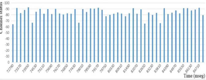
The actual sequence used to contrast the success rate in predicting channel status versus the one delivered by the DBN model is shown in Fig. 4, where the time interval of the series varies from 72,790 to 87,000 msec, a total of observations of 50 values and producing the binary string:

01011001010100001010111100000001010000010000110110

Fig. 4.Sample of actual data to be compared against the prediction given by the BN

IV. TRAINING,MODELINGANDPREDICTION.

The Bayesian network design (done on Netica software) is generated from the variables that model PU activity, and the way to identify channel usage by the licensed user is by determining the power level (dBm) existing in the spectral band; therefore the "power" variable is used as an identifier of presence/absence of PU. According to Fig. 5, the variables with their statuses that are included in the structure of the Bayesian network are:

• Delay. A predictor variable, which represents the delay in the transmission and directly affects the node

"Wifi Channel" node and is identified with “High_R” and “Low_R”statuses.

• Bandwidth. Predictor type variable, and is related to the transmission capacity of a channel; it affects

the "Wifi Channel" node and is identified with “High_BW” and “Low_BW”statuses.

• SNR. Predictor variable type; represents the Signal to Noise Ratio, and affects the "Wifi Channel" node

and is identified with “High_SNR” and “Low_SNR” statuses.

• Wifi Channel: node representing the channel status and is identified with the “Occupied” and

“Available” statuses.

• Occupied/Non-occupied Channel. Class-type Variable; represents the power used for transmission and

affects the "Modeling" node and is identified with “High” and “Low” statuses.

• Modeling. Node representing the PU use channel pattern and is identified with the “Occupied” and

“Non-Occupied” tatuses.

• Prediction. Node representing the probabilities of use or non-use of the channel and is identified with

Fig. 5. Bayesian network designed by experts

In order to interact with or without prior information of an environment and self-program to determine PU behavior (training phase), the implementation of learning algorithms that train the BN structure generating the joint probability tables (JPT) for inference, which are generated by the percentages of PU statuses in both modeling and prediction. The methodologies that can be used at each stage of BN development are TAN,EM or GD, which are explained later in this section (Fig. 6).

Fig. 6. BN for training and prediction parameters

With a trained BN, it is necessary to identify the one that best models PU behavior given the predictor variables, the class variable and the BN structure used. CO, MPE and SF methods of analysis (Fig. 6) were used to determine the BN that had better performance in representing PU dynamics.

Establishing how well adjusted a BN is to an unknown data set (rediction percentage estimate) involves using the method of cross-validation [21], [22] using punctuation rules: CM, ER, C, TS and SRLV (Fig. 6) and applying them to the methodologies TAN, EM or GD (or the one that delivered better results in the modeling

BN Structure

Training Stage

Tree Augmented Network

(TAN) Expectation Maximization (EM) Gradient Descent (GD)

Compile Optimized

(CO) Most Probable Explanation (MPE) Sensitivy to Findings (SF)

Prediction Stage

Confusion Matrix

(CM) Error Rate (ER) Calibration (C) Time Surprised (TS)

phase) [23]. For this stage, it is necessary to use a set of cases that has not been presented to the network in its learning; and this performance evaluation is applied choosing the query node of which the value of its beliefs (predictions) needs to be know during interference.

A. Tree Augmented Network (TAN).

It is an improved version of the Naive Bayes classifier and adaptation of the Chow-Li algorithm [24]. This algorithm takes into account the amount of mutual information subject to the class variable, i.e. the weight of information between the predictor variables and the class variable, without ignoring the relationship between each of the variables and ensuring a maximum of two parents for each variable, this in order to improve prediction regarding its predecessors Naïve-Bayes techniques, Bayes2, Bayes5, Bayes9, BayesN, [19, 25, 15]. The basis of the algorithm is in the use of the formula (Equation 2) of Mutual Information (MI), comparing the correlation between samples and deciding which of these contains more information about the variable class, in the end only the links that generate greater dependence between nodes will remain. In Fig. 7, the TAN technique flowchart is presented.

; ∑ ∑ , log ,

Where is the variable to evaluate, C is the class variable, is the number of statuses that can

take and is the number of statuses that the class variable can take. and are marginal probabilities and are calculated by the sum of the probabilities of all the joint events, i.e. the probability that both and

events occur together.

Fig. 7. Flowchart of TAN methodology

The steps that describe the technique behavior are [24]:

1. Calculate the Mutual Information (correlation) for each of the possible links except for the "Class2 variable.

2. Arrange the correlations from the highest to the lowest. 3. Use a node-only scheme (variables).

4. Connect the two most heavily weighted variables (links) between conditional mutual information (nodes).

5. Assign a new link given that no cycles are formed; in case of cycling, the link is dropped. 6. The above steps are run again to end links.

7. Choose a variable as the root node to direct each of the links. B. Expectation Maximization (EM).

It is an iterative parametric method that seeks maximum probability or maximum a posteriori (MAP) for the parameters in the model, these are generally useful having latent variables (variables with little or no information) using a mixed supervised learning and unsupervised model. The algorithm takes place in two steps:

Expectation Step: Estimates missing or lost data from their expected values; these are obtained using current estimates of the parameters.

Maximization Step: Calculates the parameters maximizing the probability function found in the previous step, i.e.they obtain the maximum probability estimators [25]. In Fig. 8, the flowchart of EM technique is presented.

Fig. 8.Flowchart of MS technique

The steps that describe the technique are [26]:

1. E-Step: Estimating the latent or hidden data from current data for the parameter.

2. The estimate is achieved from a conditional (threshold), which specifies the user. In order to converge to some extent to limit the threshold.

3. The result is the probability distribution function.

4. M-Step: Starts maximizing the probability function, assuming latent or hidden data are known.

5. The estimates of missing data found in the E-Step are used, making them participate as if they were real.

6. After several iterations it is converged to a maximum limited by the threshold provided by the expert. C) Gradient Descent (GD).

It is a first order parametric algorithm, used for optimization using the "gradient descent". This technique is used to find the minimums of the function evaluated, in this case those of the TPC, in contrast to the EM technique that seeks to maximize and the TAN technique looking for the posteriori probabilities from the a-priori. In this sense it seeks to explore another alternative to generate the BN that best describes the PU behavior. In Fig. 9, the GD technique flowchart is presented.

The operation of the technique is described below [27]: 1. It starts with an assumption of the solution.

2. Each variable is normalized to have a zero mean. (Normalization refers to modelling the variables to obtain a common point)

3. The data set is normalized so that there is no linear correlation between them. a. Each variable is projected onto an orthogonal base.

b. The covariance matrix is found.

c. The input data are multiplied by the matrix.

4. Each variable is normalized in order to return to the same variance. 5. A learning parameter (threshold) is chosen.

6. It is proceeded to evaluate the variances with respect to the threshold in several iterations until the minimum is reached.

a. If the convergence is very low it can be a local minimum.

Fig. 9.GD TechniqueFlowchart.

V. RESULTS

Before sharing the results obtained, it is important to clarify that the structure of the BN created was evaluated using each of the methodologies TAN, EM and GD and for each of the variables shown in Figure 6 in the training and prediction phases, however due to a lack of space in this article only the one that presents the best result in each case is presented.

A. PU Modeling.

1) Compile Optimized. When compiling the BN to form the JPT of each node, it generates a "Juntion Tree" [22], [20] internally, which is a tree-like structure that allows to update the information nodes or links, for the respective inference calculations, according to findings presented or modifications made to the BN. The intent of this method is to show the amount of memory used by each “Juntion Tree”, referring to resource consumption in a standard PC of typical configuration (Intel Core i7, 8GB RAM).

The structure generated by the training techniques did not produce a report of significant memory consumption; it was observed that the structure generated with TAN learning consumes an amount of memory of 6.04 kb and EM and GD techniques consume 4.128 kb. The difference between these amounts is currently not significant, suggesting that the BN could be implemented smoothly at a central station within a cognitive radio network.

2) Most Probable Explanation. Given the BN it is necessary to confirm that the impact between the variables from the presentation of findings (samples) in one of the nodes, i.e. if a node receives a finding of what variables (nodes) it affects directly and to what extent (level of beliefs/statuses).

From metrics included for evaluating PU modeling it is concluded that EM presents the best result for the Bayesian network because its operation is based on seeking maximum a posteriori probability of occurrence.

3) Sensitivity to Findings. What the sensitivity analysis aims is to be able to determine that both the "Class" node is influenced by the other nodes; and to determine the variance of its beliefs (i.e. establish that such dispersion have beliefs around its mean). This in order to determine the effectiveness of the response of the BN to model and predict the PUs.

Fig. 10. Comparison in time of the behavior between the actual signal and delivered by DBN

As a final result, the BN designed and trained with the EM technique was the choice with the best performance to model PU behavior, as this stood out among the other techniques delivering results according to PU behavior and the expert approach. The success rate was above 97% as shown in Fig. 10, showing a comparison (using Dynamic Bayesian Networks (DBN)) between the original data sequence and that delivered by the DBN. Fig. 11 shows a more detailed approximation thereof for a shorter time interval.

Fig. 11. Extensionof comparison between the actual signal and that delivered by DBN for modeling

B. PU Prediction.

1) Confusion Matrix. This variable relates failed and successful statuses for each belief of the chosen node. Once belief values are generated, these are compared with the actual values not included in the training stage to determine if they match, to finally generate a prediction report for the evaluated node and display them in the confusion matrix.

The results in Table III suggest that future PU channel behavior estimating is more successful with the EM and GD techniques because the success rate is closer to reality.

TABLE II. Confusión Matrix

States/Methodologies TAN EM GD

Bussy 10/1 10/1 10/1

By way of interpretation, EM in Bussy status, had 10 successes and one failure (or failures to alert); in the Idle status, 18 evaluations had no failures, indicating a fairly optimistic prediction level.

2) Error Rate. Presents the percentage of error in the prediction; this value is generated from predicting a status and not hitting the correct value. The result of this variable is shown in Table IV and it is concluded that the lowest prediction error is presented by EM and GD.

TABLE III. Prediction error in the RB

Rates/Methodologies TAN EM GD

Error rate 10.34% 3.44.% 3.44.%

3) Scoring Rule Result and Logarithmic Loss Values. Interpreted as the degree of adjustment the model has compared to the new dataset. These scoring rules deliver an optimized rating of the probabilistic prediction assigned to a set of possible outcomes; that is, a score can be considered as a measure of "calibration" of a set of probabilistic predictions, where the most commonly used are logarithmic loss, quadratic loss and spherical compensation.

The different methods in Table V show prediction scores found for the learning techniques.

TABLE IV. Scoring rules for each technique

Función/Metodologías TAN EM GD

Logarithmic loss 0.5203 1.106 0.6277 Quadratic loss 0.1702 0.0763 0.0697 Spherical loss 0.9653 0.9628 0.908

From Table V it is concluded that the calibration by the methods found in the different techniques confirm that the BN structure achieved by GD is the best for prediction because the error rates are low and it has high optimization. Note that the "Logarithmic loss" function clearly indicates that TAN and GD are the BNs showing the best performance by minimizing the error rate; the "Quadritic loss" parameter (defined in the range 0 and 2) and "Spherical payoff" (between 0 and 1) confirms that GD has the best performance in estimating a more accurate prediction because the error rate is reduced and has a high level of learning.

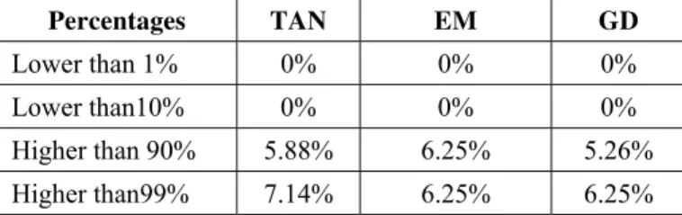
4) Time Surprised. Used to determine that the BN was quite confident in its beliefs but they were wrong. This performance index indicates how many times the system failed to predict with respect to overall executed predictions.

In defining how erroneous the prediction may be based on the beliefs associated with the "modeling" node the most favorable condition was the GD (see Table VI) due to the fact that its prediction percentage error was significantly lower than the other cases.

TABLE V. Confidence events delivered by each technique

Percentages TAN EM GD

Lower than 1% 0% 0% 0%

Lower than10% 0% 0% 0%

Higher than 90% 5.88% 6.25% 5.26% Higher than99% 7.14% 6.25% 6.25%

is shown in Fig. 12, which contains the 50 events presented by predicting BN (blue) and 25% of the capture which corresponds to the actual model (orange); the red line refers to the threshold (-89 dBm) selected to determine whether the channel is busy or not. The results provided by the BN indicate that for a value above 96.56% of the samples collected correctly predict the PU activity(value which will be decremented as time elapses). It may be shown that for this case there are false alerts at 73,660, 77,430, 79,460, 86,420 and 86,710milliseconds. It should be noted that the prediction made by the BN in both cases is done by calculating the percentage of belief for each event consulted.

Fig. 12. Comparison of PU prediction level between the actual signal and that delivered by DBN as a function of time

VI. CONCLUSIONS

Using Bayesian networks without depending on the structure achieved does improve CR performance, as they provide 80% success rate in modeling PU activity.

The prediction achieved by Bayesian networks for the sequence used in research exceeds 80% success rate, indicating that the artificial intelligence technique as a predictor model, could come to provide a higher level of characterization in PU and CR performance; however it is necessary to try with another type of data streams.

PU characterization contributes to decision-making in cognitive radio wireless networks, the deployment of a predictive model that could improve the level of access to licensed bands for secondary users.

Consumption of resources in a CR device by BNs (complexity) is very low compared to probabilistic and statistical predictors, so its implementation is feasible in a transmission base station.

BN learning through training techniques attempts to model the real system, but the participation of the expert is necessary to focus on the use of the BN for its specific use, which is to characterize the PU.

REFERENCES

[1] B. Canberk, Ian F. Akyildiz, S. Oktug., A QoS-aware framework for available spectrum characterization and decision in cognitive

radio networks. IEEE 21st International Symposium on Personal Indoor and Mobile Radio Communications (PIMRC), pp. 1533-1538, doi: 10.1109/pimrc.2010.5671959, Istanbul,September 26-30, 2010.

[2] J. Aguilar, Radio cognitiva-estado del arte, Revista Sistemas y Telemática, Universidad ICESI, Vol. 9, Nº 16, pp. 31-53. [Online],

available: https://www.icesi.edu.co/revistas/index.php/sistemas_telematica/article/viewFile/1028/1053.

[3] W. Saad, z. Han, H. Poor, T. Basar, J. Song, A cooperative Bayesian nonparametric framework for primary user activity monitoring in

cognitive radio networks, IEEE Journal on Selected Areas in Communications, Vol 30, Nº 9, pp. 1815–22, October 2010.

[4] H. Li R. Qiu, A graphical framework for spectrum modeling and decision making in cognitive radio networks, IEEE Global

Telecommunications Conference (GLOBECOM), pp. 1–6, doi: 10.1109/glocom.2010.5683361, Miami, December 6-10, 2010.

[5] J. Mitola, G. Maguire, Cognitive radio: making software radios more personal, IEEE Personal Communications, Vol 6, N° 4, pp.

13-18, 1999.

[6] M. Bkassiny, L. Yang, S. Jayaweera, A survey on machine-learning techniques in cognitive radios, IEEECommunications Surveys &

Tutorials, Vol 15, N° 3, pp. 1136-1159, 2013.

[7] U. Berthold, F. Fu, M. Schaar, F. Jondral, Detection of spectral resources in cognitive radios using reinforcement learning, IEEE

Symposium onNew Frontiers in Dynamic Spectrum Access Networks, DySPAN, pp. 1-5, doi: 10.1109/dyspan.2008.82, Chicago,

October 14-17, 2008.

[8] N. Baldo, B. Tamma, B. Manoj, R. Rao, M. Zorzi, A neural network based cognitive controller for dynamic cannel selection, IEEE

International Conference on Communications, pp. 1-5, doi: 10.1109/icc.2009.5198636, Dresden, June 14-18, 2009.

[9] A. He, K. Bae, T. Newman, J. Gaeddert, k. Kim, R. Menon, L. Tirado, J. Neel, Y. Zhao, J. Reed, W. Tranter, A survey of artificial

intelligence for cognitive radios, IEEE Transactions on Vehicular Technology, Vol 59, N° 4, pp. 1578-1592, 2010.

[10] K. Haghighi, Model based cognitive radio strategies, Thesis for the degree of Doctor of Philosophy, Department of Signal and Systems, Chalmers University of Technology, Gothenburg, Gothenburg (Sweden), 2013. [Online], available: http://publications.lib.chalmers.se/records/fulltext/183611/183611.pdf.

[11] M. Puterman, Markov Decision Processes: Discrete Stochastic Dynamic Programming, Ed. Wiley, pp. 20-25, ISBN:

978-0471-72782-8, New York (USA), 2005.

[12] B. Canberk, I. Akyildiz, S. Oktug, Primary user activity modeling using first-difference filter clustering and correlation in cognitive

radio networks,IEEE/ACM Transactions on Networking (TON), Vol 19, N° 1, pp. 170-183, February 2011.

[13] R. Streit, Poisson point processes, Ed. Wiley, pp. 38-53, ISBN: 978-1441969224, Virginia (USA), 2010.

[14] D. Montgomery, C. Jennings, M. Kulahei, Introduction to time series analysis and forecasting, Second edition, Ed. Wiley, pp. 80-95,

[15] U. Kjaerulff, A. Madsen, Bayesian networks and influence diagrams: A guide to construction and analysis, Second edition, Ed. Springer, pp. 69-299, ISBN: 978-1-4614-5104-4, New York (USA), 2013.

[16] M. Scutari, J-B. Denis, Bayesian networks with examples in R, Ed. CRC Press, pp. 11-172, ISBN: 978-1-14822-2558-7, USA, 2014.

[17] L. Husheng, Qiu. R, A graphical framework for spectrum modeling and decision making in cognitive radio networks, IEEE Global

Telecommunications Conference (GLOBECOM), pp. 1–6, doi: 10.1109/glocom.2010.5683361, Miami, December 6-10, 2010.

[18] J. Pearl, Causality: Models, reasoning, and inference, Cambridge University Press, pp. 65-130, ISBN: 978-0521773621, Los Angeles

(USA), 2000.

[19] N. Ramirez, Building Bayesian networks from data: A constraint based approach, Thesis for the degree of Doctor of Philosophy,

Department of Psychology, University of Sheffield, UK, 2001. [Online], available:

http://cdigital.uv.mx/bitstream/123456789/29390/1/Cruz%20Ramirez.pdf

[20] K. Korb, A. Nicholson, Bayesian artificial intelligence, Computer Science and Data Analysis Series, Second edition, pp. 29-50, ISBN:

978-1439815915, UK, 2010.

[21] Y. Mancilla, Caracterización de usuarios WiFi para redes de radio cognitiva, Thesis for the degree of Master, Faculty of Engineering,

University Distrital Francisco José de Caldas, Bogotá (Colombia), 2015.

[22] Software Netica, 2016. [Online], available: http://www.norsys.com/WebHelp/NETICA.htm.

[23] A. Darwiche, Modeling and reasoning with Bayesian Networks, Cambridge University Press, pp. 53-122, ISBN: 978-0521884389,

New York, 1999.

[24] C. Chow, C. Liu, C.N, Approximating discrete probability distributions with dependence trees, IEEE Transactions on Information Theory, Vol 14, N° 3, pp. 462–467, 1968.

[25] N. Friedman, D. Geiger, M Goldszmidt, M, Bayesian network classifiers, JournalMachine learning, Springer, Vol29, N° 2-3, pp.

131-163, doi: 10.1023/A:1007465528199, 1997.

[26] P. Dempster, N. Laird, D. Rubin, Maximum likelihood from incomplete data via the EM algorithm, Journal of the Royal Statistical

Society: Series B, Vol 39, N° 1, pp. 1–38, 1977.

[27] F. Jensen, Gradient descent training of Bayesian networks, European Conference on Symbolic and Quantitative Approaches to