ensembles, and gene expression data analysis
SERVIÇO DE PÓS-GRADUAÇÃO DO ICMC-USP
Data de Depósito:
Assinatura:______________________
Pablo Andretta Jaskowiak
On the evaluation of clustering results: measures,
ensembles, and gene expression data analysis
Doctoral dissertation submitted to the Instituto de Ciências Matemáticas e de Computação - ICMC-USP, in partial fulfillment of the requirements for the degree of the Doctorate Program in Computer Science and Computational Mathematics. FINAL VERSION
Concentration Area: Computer Science and Computational Mathematics
Advisor: Prof. Dr. Ricardo José Gabrielli Barreto Campello
Coadvisor: Prof. Dr. Ivan Gesteira Costa
Ficha catalográfica elaborada pela Biblioteca Prof. Achille Bassi e Seção Técnica de Informática, ICMC/USP,
com os dados fornecidos pelo(a) autor(a)
A555o
Andretta Jaskowiak, Pablo
On the evaluation of clustering results: measures, ensembles, and gene expression data analysis / Pablo Andretta Jaskowiak; orientador Ricardo José Gabrielli Barreto Campello;
co-orientador Ivan Gesteira Costa. -- São Carlos, 2015. 152 p.
Tese (Doutorado - Programa de Pós-Graduação em Ciências de Computação e Matemática Computacional) Instituto de Ciências Matemáticas e de Computação, Universidade de São Paulo, 2015.
1. cluster analysis. 2. clustering. 3.
Pablo Andretta Jaskowiak
Sobre a avaliação de resultados de agrupamento:
medidas, comitês e análise de dados de expressão gênica
Tese apresentada ao Instituto de Ciências Matemáticas e de Computação - ICMC-USP, como parte dos requisitos para obtenção do título de Doutor em Ciências - Ciências de Computação e Matemática Computacional. VERSÃO REVISADA Área de Concentração: Ciências de Computação e Matemática Computacional
Orientador: Prof. Dr. Ricardo José Gabrielli Barreto Campello
Coorientador: Prof. Dr. Ivan Gesteira Costa
the winning tickets are visible.
Jostein Gaarder
Acknowledgements
A minha querida e amada m˜ae, Lidete Maria Andretta, que sempre me apoiou incondicionalmente durante toda esta jornada. Sem seu amor, carinho e suporte (inclusive
financeiro) eu n˜ao teria chegado at´e aqui. Obrigado por se fazer presente em toda minha vida.
Ao meu orientador, Prof. Ricardo J. G. B. Campello, que teve papel fundamental no meu
crescimento pessoal e profissional, desde o meu mestrado. Sua dedicac¸˜ao e constante busca pela
excelˆencia s˜ao inspirac¸˜oes que levo comigo para toda a vida, n˜ao s´o a acadˆemica.
Ao meu co-orientador, Prof. Ivan G. Costa, excelente profissional pelo qual tenho grande
admirac¸˜ao, que mesmo distante fisicamente, esteve sempre presente ao longo deste trabalho
enriquecendo todas nossas discuss˜oes. Meu obrigado tamb´em pela sua recepc¸˜ao na Universidade
Federal de Pernambuco (UFPE) durante os dois mesˆes em que estive visitando seu laborat´orio. Ao Prof. J¨org Sander, por me receber sob sua supervis˜ao durante um ano na Universidade de
Alberta (U of A), em Edmonton, AB, Canad´a. Meu obrigado tamb´em aos amigos Arthur Zimek e
Davoud Moulavi, com quem tive o privil´egio de colaborar neste per´ıodo e dividir alguns pistaches.
A todos amigos e amigas do laborat´orio Biocom, pelas calorosas discuss˜oes cient´ıficas (ou
n˜ao) e por toda a convivˆencia extra laborat´orio. Extendo os agradecimentos a todos os amigos e
amigas que fiz em S˜ao Carlos em todos esses anos. Os palquinhos e churrascos trar˜ao saudades. A
Amanara Potykyt˜a, por todo seu amor, calma e compreens˜ao, vocˆe tornou tudo mais f´acil.
Sou grato tamb´em aos membros do comitˆe avaliador, Prof. Wagner Meira J´unior, Prof. Renato
Tin´os, Prof. Ana Carolina Lorena e Prof. Alexandre Cl´audio Botazzo Delbem, por seu tempo e suas considerac¸˜oes e contribuic¸˜oes ao trabalho. Elas est˜ao refletidas nesta vers˜ao do texto.
A Fundac¸˜ao de Amparo `a Pesquisa do Estado de S˜ao Paulo (FAPESP), pelo suporte financeiro
ao projeto, tanto de bolsa regular de doutorado (Processo FAPESP #2011/04247-5) quanto
de est´agio de pesquisa no exterior (Processo FAPESP #2012/15751-9) e a Coordenac¸ao de
Aperfeic¸oamento de Pessoal de N´ıvel Superior (CAPES) pelo aux´ılio financeiro inicial ao projeto.
Abstract
C
lustering plays an important role in the exploratory analysis of data. Its goal is to organize objects into a finite set of categories, i.e., clusters, in the hope that meaningful and previously unknown relationships will emerge from the process. Not every clusteringresult is meaningful, though. In fact, virtually all clustering algorithms will yield a result,
even if the data under analysis has no “true” clusters. If clusters do exist, one still has to
determine the best configuration of parameters for the clustering algorithm in hand, in order to
avoid poor outcomes. This selection is usually performed with the aid of clustering validity
criteria, which evaluate clustering results in a quantitative fashion. In this thesis we study the
evaluation/validation of clustering results, proposing, in a broad context, measures and relative
validity criteria ensembles. Regarding measures, we propose the use of the Area Under the
Curve (AUC) of the Receiver Operating Characteristics (ROC) curve as a relative validity criterion for clustering. Besides providing an empirical evaluation of AUC, we theoretically explore some
of its properties and its relation to another measure, known as Gamma. A relative criterion for
the validation of density based clustering results, proposed with the participation of the author of
this thesis, is also reviewed. In the case of ensembles, we propose their use as means to avoid the
evaluation of clustering results based on a single, ad-hoc selected, measure. In this particular scope,
we: (i) show that ensembles built on the basis of arbitrarily selected members have limited practical
applicability; and (ii) devise a simple, yet effective heuristic approach to select ensemble members,
based on their effectiveness and complementarity. Finally, we consider clustering evaluation in
the specific context of gene expression data. In this particular case we evaluate the use of external
information from the Geno Ontology for the evaluation of distance measures and clustering results.
keywords: clustering, clustering validation
Resumo
T
dados. Seu objetivo ´e a organizac¸˜ao de objetos em um conjunto finito de categorias,´ecnicas de agrupamento desempenham um papel fundamental na an´alise explorat´oria de i.e., grupos (clusters), na expectativa de que relac¸˜oes significativas entre objetos resultemdo processo. Nem todos resultados de agrupamento s˜ao relevantes, entretanto. De fato, a vasta
maioria dos algoritmos de agrupamento existentes produzir´a um resultado (partic¸˜ao), mesmo em
casos para os quais n˜ao existe uma estrutura “real” de grupos nos dados. Se grupos de fato existem,
a determinac¸˜ao do melhor conjunto de parˆametros para estes algoritmos ainda ´e necess´aria, a fim
de evitar a utilizac¸˜ao de resultados esp´urios. Tal determinac¸˜ao ´e usualmente feita por meio de crit´erios de validac¸˜ao, os quais avaliam os resultados de agrupamento de forma quantitativa. A
avaliac¸˜ao/validac¸˜ao de resultados de agrupamentos ´e o foco desta tese. Em um contexto geral,
crit´erios de validac¸˜ao relativos e a combinac¸˜ao dos mesmos (ensembles) s˜ao propostas. No que
tange crit´erios, prop˜oe-se o uso da ´area sob a curva (AUC —Area Under the Curve) proveniente
de avaliac¸˜oes ROC (Receiver Operating Characteristics) como um crit´erio de validac¸˜ao relativo no
contexto de agrupamento. Al´em de uma avaliac¸˜ao emp´ırica da AUC, s˜ao exploradas algumas de
suas propriedades te´oricas, bem como a sua relac¸˜ao com outro crit´erio relativo existente, conhecido
como Gamma. Ainda com relac¸˜ao `a crit´erios, um ´ındice relativo para a validac¸˜ao de resultados de
agrupamentos baseados em densidade, proposto com a participac¸˜ao do autor desta tese, ´e revisado. No que diz respeito `a combinac¸˜ao de crit´erios, mostra-se que: (i) combinac¸˜oes baseadas em uma
selec¸˜ao arbitr´aria de ´ındices possuem aplicac¸˜ao pr´atica limitada; e (ii) com o uso de heur´ısticas
para selec¸˜ao de membros da combinac¸˜ao, melhores resultados podem ser obtidos. Finalmente,
considera-se a avaliac¸˜ao/validac¸˜ao no contexto de dados de express˜ao gˆenica. Neste caso particular
estuda-se o uso de informac¸˜ao da Gene Ontology, na forma de similaridades semˆanticas, na
avaliac¸˜ao de medidas de dissimilaridade e resultados de agrupamentos de genes.
palavras chave: agrupamento de dados, validac¸˜ao de agrupamentos
Contents
Acknowledgements i
Abstract iii
Resumo v
List of Figures xi
List of Tables xiii
Notation xv
List of Abbreviations xvii
1 Introduction 1
1.1 Contributions . . . 4
1.2 Outline . . . 5
2 Cluster Analysis 7 2.1 Basic Concepts . . . 7
2.2 Clustering Algorithms . . . 10
2.2.1 k-means and k-medoids . . . 10
2.2.2 Hierarchical Clustering Algorithms . . . 11
2.2.3 DBSCAN . . . 12
2.3 Clustering Validation . . . 13
2.3.1 External Validation . . . 14
2.3.2 Internal and Relative Validation . . . 15
2.4 Relative Validity Criteria Evaluation . . . 20
2.4.1 Traditional Methodology . . . 20
2.4.2 Alternative Methodology . . . 21
2.5 Chapter Remarks . . . 22
3 Gene Expression Data 23 3.1 Biological Background . . . 24
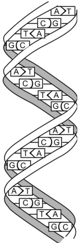
3.1.1 Nucleic Acids . . . 24
3.1.2 Gene Expression . . . 25
3.2 Measuring Gene Expression . . . 26
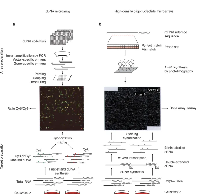
3.2.1 Microarrays . . . 27
3.2.2 RNA-Seq . . . 28
3.3 Clustering Gene Expression Data . . . 30
3.4 Gene Ontology . . . 32
3.5 Chapter Remarks . . . 34
4 Ensembles for Relative Validity Criteria Evaluation 35 4.1 Related Work . . . 37
4.2 Random Selection of Ensemble Members . . . 38
4.2.1 Experimental Setup . . . 39
4.2.2 Results and Discussion . . . 42
4.3 Heuristic Selection of Ensemble Members . . . 46
4.3.1 Combination Strategies . . . 47
4.3.2 Selecting Relative Criteria . . . 51
4.3.3 Experimental Setup . . . 56
4.3.4 Results and Discussion . . . 57
4.4 Chapter Remarks . . . 61
5 Relative Validation of Clustering Results 63 5.1 ROC Curves in Clustering Validation . . . 64
5.1.1 Basic Concepts . . . 64
5.1.2 AUC as a Relative Validity Criterion . . . 65
5.1.3 Equivalence Between AUC and Baker and Hubert’s Gamma . . . 69
5.1.4 Experimental Evaluation . . . 71
5.2 Validation of Density-Based Clustering Solutions . . . 74
5.2.1 Related Work . . . 74
5.2.2 Density-Based Clustering Validation . . . 75
5.2.3 Adapting Relative Validity Criteria to Handle Noise . . . 77
5.2.4 Experimental Evaluation . . . 78
5.3 Chapter Remarks . . . 82
6.1 Related Work . . . 85
6.2 Distance Measures . . . 86
6.2.1 Classical Measures . . . 86
6.2.2 Correlation Coefficients . . . 87
6.2.3 Time-Course Specific Measures . . . 89
6.3 Distance Measures Evaluation . . . 91
6.3.1 Clustering Algorithm Independent . . . 91
6.3.2 Clustering Algorithm Dependent . . . 96
6.4 Experiments on Microarray Data . . . 97
6.4.1 Experimental Setup . . . 97
6.4.2 Results and Discussion . . . 99
6.5 RNA-Seq Data . . . 110
6.5.1 Experimental Setup . . . 110
6.5.2 Results and Discussion . . . 111
6.6 Chapter Remarks . . . 117
7 Biological Validation of Gene Clustering Results 119 7.1 Related Work . . . 120
7.2 Gene Ontology Similarities in Relative Validation . . . 122
7.2.1 Results and Discussion . . . 122
7.3 Undesired Properties of the BHI . . . 125
7.4 Chapter Remarks . . . 127
8 Conclusions 129 8.1 Future Work . . . 130
8.2 Publications . . . 131
References 135
List of Figures
2.1 Result from a Hierarchical Clustering Algorithm. . . 9
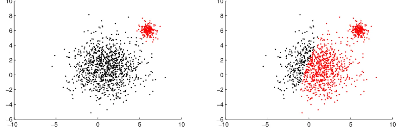
2.2 Two partitions of the same data, withk= 2clusters, denoted in red and black. . . . 22
3.1 Representation of a double stranded DNA molecule. . . 25
3.2 The central dogma of molecular biology . . . 26
3.3 Manufacture and experimental processes for Affymetrix and cDNA microarrays. . 29
3.4 Depiction of a gene expression data matrix. . . 31
3.5 Example of relations between terms in the Gene Ontology . . . 33
4.1 Three complementary relative validity criteria in a binary evaluation scenario. . . . 36
4.2 Average effectiveness of each individual relative validity criterion. . . 52
4.3 Complementary Assessment for the 28 relative criteria. . . 53
4.4 Results for ensembles built with relative criteria subsets selected with our approach. 55 4.5 Results for ensembles selected with our heuristic, single criterion, and random. . . 60
4.6 Effectiveness of all the ensembles built. . . 61
5.1 An example of ROC Graph for different classifiers. . . 66
5.2 Evaluation of AUC/Gamma and other 28 relative validity criteria. . . 72
5.3 Results regarding the evaluation of randomly generated partitions. . . 73
5.4 Synthetic datasets employed during DBCV evaluation . . . 79
5.5 Results for the best measures regarding synthetic datasets. . . 81
6.1 Intrinsic Separation Ability (ISA) for each one of the evaluated distances. . . 100
6.2 Intrinsic Separation Ability (ISA) regarding different noise levels. . . 101
6.3 Intrinsic Biological Separation Ability (IBSA) for each one of the distances. . . 101
6.4 Intrinsic Biological Separation Ability (IBSA) regarding different noise levels. . . . 103 6.5 Class recovery obtained for cancer datasets regarding the three evaluation scenarios. 105
6.6 Robustness to noise regarding cancer datasets. . . 106
6.7 Results obtained for the clustering of gene time-series data. . . 108
6.8 RNA-Seq clustering decision pipeline. . . 112
6.9 Results for genes (RSEM), considering 1K features. . . 114 6.10 Results for genes (RPKM), with 1K features. . . 115
7.1 Results regarding relative evaluation based on the GO. . . 124
7.2 Relative validation: biological, statistical, and combined forelutriationdataset. . . 125
7.3 Examples regarding cluster homogeneity and completeness properties. . . 126
List of Tables
2.1 Distances between clusters commonly used in HCAs. . . 11
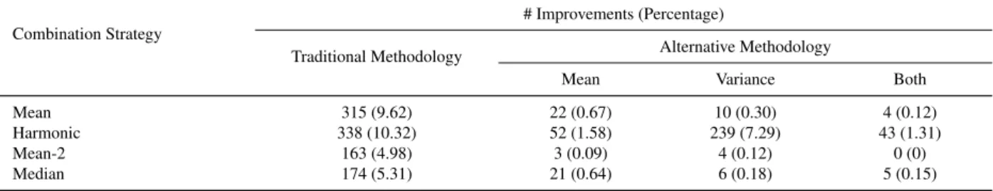
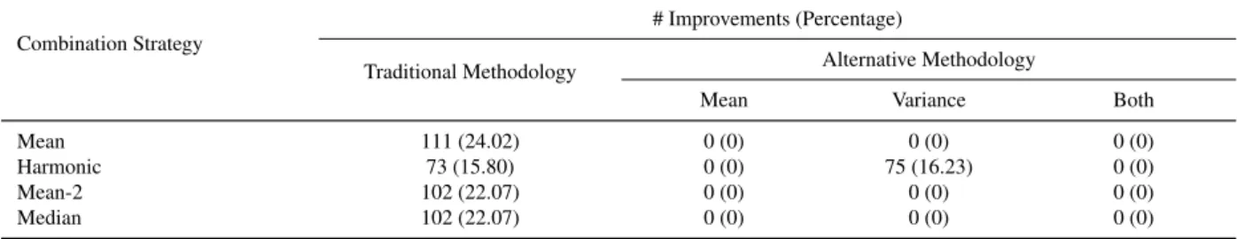
4.1 Improvements over all the individual criteria involved in the combination (nc = 3) . 42
4.2 Improvements over at least one of the criteria involved in the combination (nc = 3). 43
4.3 Improvements over all the three criteria involved in the combination. . . 44
4.4 Improvements over at least one of the criteria involved in the combination (nc = 3). 44
4.5 Improvements over all the five criteria involved in the combination. . . 44
4.6 Improvements over at least one of the criteria involved in the combination (nc = 5). 44
4.7 Results for the selected criteria subsets. . . 57
4.8 Effectiveness (correlation w.r.t. external index) of individual relative validity criteria. 58
4.9 Effectiveness for the best performing criteria subset selected with our approach. . . 59
5.1 Best Adjusted Rand Index (ARI) value found for each relative validity criterion. . . 80
5.2 Spearman correlation with respect to the external validity index (ARI). . . 82
6.1 Cancer microarray datasets used in the experiments. . . 98 6.2 Time-course microarray datasets used in the experiments. . . 98
6.3 Statistical Test Summary - MF and BP Ontologies. . . 102
6.4 Wins/Ties/Losses for 15 distances and 17 datasets. . . 107
6.5 TCGA Datasets Summary. Main characteristics of the datasets under analysis. . . . 110
Notation
This document adopts the following convention:
• Scalars are given in lower case italics;
• Vectors are given in lower case bold;
• Matrices are given in upper case bold;
• Sets are given in upper case italics.
Notation is as follows:
|.| The cardinality of a given set X A set of objects,i.e., a dataset
n The number of objects inX,i.e.,|X|
xi An object fromX,i.e., am-dimensional vectorxi= (x1, . . . , xm) m The number of dimensions (i.e., features) for a given object or dataset
C A set ofk clusters,i.e., a clustering or partition, withC ={Ci, . . . , Ck}
ci The centroid from clusteri
D A dissimilarity matrix
k Number of clusters
k∗ Theoptimal(desired) number of clusters as defined by a reference partition
kmax The superior limit considered for the cluster number, typicallykmax =⌈√n⌉
Lista de Abreviaturas
ALOI Amsterdam Library of Object Images
AL Average-Linkage
ARI Adjusted Rand Index
ASSWC Alternative Simplified Silhouette Width Criterion
ASWC Alternative Silhouette Width Criterion
AUC Area Under the Curve
BP Base Pairs
cDNA Complementary Deoxyribonucleic Acid
CL Complete-Linkage
DBCV Density Based Clustering Validation
DBSCAN Density-Based Spatial Clustering of Applications with Noise
DB Davies-Boudlin (Criterion)
DNA Deoxyribonucleic Acid
FN False Negative
FP False Positive
HCAs Hierarchical Clustering Algorithms
IBSA Intrinsic Biological Separation Ability
ISA Intrinsic Separation Ability
mRNA Messenger Ribonucleic Acid
PBM Pakhira, Bandyopadhyay, and Maulik’s (Criterion)
PB Point-Biserial (Criterion)
PCA Principal Component Analysis
PCR Polymerase Chain Reaction
RI Rand Index
RNA Ribonucleic Acid
ROC Receiver Operating Characteristics
rRNA Ribosomal Ribonucleic Acid
SL Single-Linkage
SSE Sum of Squared Errors
SSWC Simplified Silhouette Width Criterion
SWC Silhouette Width Criterion
TIFF Tagged Image File Format
TN True Negative
TP True Positive
tRNA Transfer Ribonucleic Acid
VRC Variance Ratio Criterion
1
Introduction
We are embedded in a world of data. As our capacity to collect and store data from the most varied sources continues to evolve, so does the need of developing efficient methods to analyze and
extract useful information from them. The field of Data Mining embraces methods and algorithms
from different areas of research, such as Artificial Intelligence, Machine Learning, and Statistics,
that aim to uncover valuable information from data (Fayyad et al., 1996; Tan et al., 2006). Its
methods are usually categorized into different tasks, which can be broadly regarded as supervised
and unsupervised, taking into account the learning strategy they employ (Tan et al.,2006).
Cluster analysis, or simply clustering, is an unsupervised Data Mining task. Given that no
prior knowledge is used during the clustering process, it finds great applicability in the exploratory
analysis of data. Its goal is to organize data objects into a finite set of categories, i.e., clusters,
by abstracting the underlying structure of the data, in the hope that meaningful and previously
unknown relationships among objects will emerge as a result of the process (Hartigan,1975;Jain
and Dubes, 1988). The lack of a globally accepted definition for the term cluster in the literature
drove the development of several clustering paradigms and numerous clustering algorithms within each paradigm (Estivill-Castro,2002;Jain and Dubes,1988). These have been applied to the most
diverse areas of expertise, such as astronomy, economics, psychology, and bioinformatics, just to
mention a few (Jain,2010;Tan et al.,2006;Xu and Wunsch II,2009;Zhang,2006).
One of the first steps of the clustering procedure is to choose an adequate clustering
algorithm and set its parameters properly for the application in hand. The choice of a
particular algorithm and its corresponding parameterization, the so-called model selection
2
problem, is, however, far from trivial in an unsupervised environment. Fortunately, over the past
years a number of mathematical indexes that can be used to guide these choices in a quantitative
way have been developed. In the clustering literature, these indexes are usually referred to
as clustering validity criteria, as they can also be used to evaluate/validate the relevance of the clustering results from a statistical perspective (Jain and Dubes, 1988; Xu and Wunsch II,
2009). In real world applications, clustering validity criteria known as internal and relative find
broad applicability. In brief, internal criteria quantify the quality of a clustering solution using only
the data itself, whereas relative criteria are internal measures that can go further and also compare
two clustering structures, pointing out which one is better, in relative terms. Although a few
exceptions do exist, these criteria are often based on the general idea of measuring, somehow, the
balance between within-cluster scattering (compactness) and between-cluster spread (separation),
with differences arising mainly from different formulations of these two fundamental concepts.
The validation of clustering results has been historically described as challenging (Milligan and Cooper,1985). Indeed, in their classical book on clustering,Jain and Dubes(1988) state that:
“The validation of clustering structures is the most difficult and frustrating part of cluster
analysis. Without a strong effort in this direction, cluster analysis will remain a black
art accessible only to those true believers who have experience and great courage.”
After almost 30 years and despite achievements observed in this particular area, we believe that the
above statement remains true. This has motivated us to study, develop, and propose methods to the evaluation of clustering results. In the general1 context of clustering validation this thesis follows
two main lines of investigation. The first one comprises the study and development of new relative
validity measures, whereas in the second one we investigate and propose the use of ensembles of
relative validity criteria, based on a careful selection of members.
With respect to measures, we propose the application of concepts from the supervised domain
of classification to the relative validation of clustering results. More specifically, we study and
adapt the Area Under the Curve (AUC) of the Receiver Operating Characteristics (ROC) curve to
the validation of clusterings. We then investigate some of its theoretical properties, and provide an
empirical evaluation of the measure. This leads to our first research hypothesis, as stated below:
• Hypothesis 1: The Area Under the Curve of the Receiver Operating Characteristics curve,
which is commonly adopted in the supervised learning setting (Fawcett, 2006), can be
effectively employed in the unsupervised setting, as a relative validity criterion.
Still regarding measures, a relative criterion for the validation of density based clustering results, proposed with the participation of the author of this thesis (Moulavi et al.,2014), is also reviewed.
Regarding ensembles, our second line of investigation, we start by acknowledging that there is
a plethora of relative validity criteria proposed in the literature (Vendramin et al.,2009,2010). The
variety of measures by itself suggests that a single evaluation index cannot capture all the aspects
involved in the clustering problem and, therefore, may fail in particular application scenarios. In
fact, due to the subjective nature of the problem, it is well-known that no index can systematically
outperform all the others in all scenarios. As conjectured by Bezdek and Pal (1998), a possible approach to bypass the selection of a single relative validity criterion is to rely on multiple
criteria in order to obtain more robust evaluations. The rationale behind this approach follows
essentially the same intuitive idea of combining multiple experts into a committee so as to get more
stable and accurate recommendations, which has been well studied in the realm of ensembles for
classification (Rokach,2010), clustering (Ghosh and Acharya,2011), and outlier detection (Zimek
et al.,2013), for instance. The belief that this topic has not received sufficient attention considering
the validation of clustering results has motivated the formulation of the following hypotheses:
• Hypothesis 2:Ensembles of relative validity criteria built on the basis of an ad-hoc selection
of their constituent members provide very limited (if any) practical benefits.
• Hypothesis 3: Ensembles built on the basis of a simple, yet principled selection of their
constituent members, perform better than those built in an ad-hoc fashion and provide more
reliable evaluations than the ones obtained with individual relative validity criteria.
The previous hypotheses are formulated in a broad sense, that is, with no particular application
domain in mind. Some application domains, however, provide peculiar challenges that require custom tailored developments. This is the case of the clustering of gene time-series, coming
from gene expression experiments (Zhang, 2006). In this particular domain, one can hardly
find externally labeled datasets for the empirical evaluation of clustering algorithms and methods.
Moreover, due to their peculiar characteristics, custom distance measures have also been developed
in the past years,e.g., (Balasubramaniyan et al.,2005;M¨oller-Levet et al.,2005), but no systematic
evaluation of them has been provided in the literature. This has motivated us to investigate
the use of biological information from the Gene Ontology (GO) (Ashburner et al., 2000) to the
evaluation of distance measures and clustering results in this particular domain. These two lines
of investigation are summarized below by two different hypotheses.
• Hypothesis 4: External information, in the form of semantic similarities extracted from
the Gene Ontology (Ashburner et al.,2000), can be employed to evaluate the suitability of
distances among pairs of gene time-series for the task of clustering, independently from the bias of a particular clustering algorithm.
• Hypothesis 5: External information, in the form of semantic similarities extracted from
the Gene Ontology (Ashburner et al., 2000), can be employed in the relative evaluation of
clustering results, whether alone or combined with statistical similarities from the data.
The assessment of the aforementioned hypotheses was carried out through empirical analysis,
4 1.1. CONTRIBUTIONS
1.1
Contributions
With the previous hypotheses in mind, the contributions of this thesis are summarized below.
1. Empirical evaluation of ad-hoc ensembles of relative validity criteria, showing that, in
general, arbitrary ensembles provide poor performance, with very limited practical benefits.
2. Proposal of a heuristic approach for building effective ensembles of relative validity criteria,
showing that ensembles derived from our heuristic provide superior results than ad-hoc ones.
These also provide more robust evaluations than those obtained with single validity criteria.
3. A review of different approaches that can be employed to combine relative validity criteria
outcomes into ensembles. These fall under two categories, namely, value and rank based.
4. The proposition of the Area Under the Curve (AUC) of the Receiver Operating Characteristics (ROC) curve as a relative validity criterion for evaluating clustering results.
5. Formal proofs regarding: (i) the expected value of the AUC; and (ii) the relation between
AUC and the Gamma Index (Baker and Hubert, 1975). Regarding (ii), we reduced the
computational time required to compute Gamma from O(n2m + n4/k) to O(n2logn),
wherenis the number of objects,mis the number of features, ankis the number of clusters.
6. An empirical evaluation of AUC/Gamma, showing that it ranks among the best alternatives
regarding a comprehensive pool of relative validity criteria. Given its reduced computational
cost and reasonable overall results, AUC/Gamma arises as an useful and viable alternative to the clustering practitioner, specially in the relational clustering setting.
7. A review of 15 distances for the clustering of gene expression data, including, for the first
time, a collection of distances specifically developed for the clustering of gene time-series.
8. The proposal of a methodology that uses biological information to the evaluation of distance
measures regarding gene time-series, namely Intrinsic Biological Separation Ability (IBSA).
9. Investigation on the use of biological information, in the form of semantic similarities
extracted from the Gene Ontology, in the relative evaluation of gene clustering results.
10. The evaluation of distance measures for the clustering of gene expression data,
w.r.t.: (i) different methodologies; (ii) robustness to noise; and (iii) considering different gene
expression data obtained with different technologies, namely, microarrays and RNA-Seq.
11. Empirical evaluation of different factors and their respective effects in the clustering of
cancer samples from RNA-Seq data, covering: (i) expression estimates, (ii) number of
1.2
Outline
This thesis is structured in eight chapters. The remainder of the thesis is organized as follows:
• Chapter 2 - Cluster Analysis: The basic concepts of cluster analysis are presented.
Classical clustering algorithms from the literature (employed in this thesis) are briefly
reviewed. The issue of clustering validation is addressed, with emphasis on relative validity
criteria. A review of procedures for the evaluation of relative validity criteria is provided.
• Chapter 3 - Gene Expression Data: Key biological concepts to the understanding of gene
expression data are reviewed. High throughput technologies employed to measure gene
expression are presented, namely microarrays and RNA-Seq. The chapter closes with a
discussion on the importance of clustering in the analysis of gene expression data.
• Chapter 4 - Ensembles for Relative Validity Criteria Evaluation: Relative validity
criteria ensembles are investigated. Ensembles built in an ad-hoc fashion are discussed
and evaluated. A principled heuristic strategy for the selection of ensemble members,
based on concepts of effectiveness and complementarity, is developed and assessed
experimentally. The developments and results from this particular chapter have already been
published, please see (Vendramin et al.,2013) and (Jaskowiak et al.,2015).
• Chapter 5 - Relative Validation of Clustering Results: Two contributions regarding the
relative validation of clustering results are presented. In the first half of the chapter, the Area
Under the Curve (AUC) of the Receiver Operating Characteristics (ROC) is introduced as a
relative validity criterion. Properties of the AUC of a clustering solution and its relation to the Gamma index (Baker and Hubert,1975) are theoretically explored. An empirical analysis of
AUC is also provided. In the remaining of the chapter, a relative validity criterion (DBCV
-Density Based Clustering Validation) proposed to the validation of density-based clustering
results is reviewed. The work regarding DBCV was performed in collaboration with Davoud
Moulavi (main contributor), during the author’s one year internship at the University of
Alberta, Edmonton, Alberta, Canada, under the supervision of Prof. J¨org Sander. Results
from the second part of this chapter have already been published, see (Moulavi et al.,2014).
• Chapter 6 - Distances for Clustering Gene Expression Data: The selection of distance
measures in the context of gene expression data clustering is addressed. A total of 15
distances are reviewed. Methodologies for the evaluation of distance measures are discussed.
A methodology that employs biological information from the Gene Ontology (Ashburner
et al., 2000) to evaluate distances between pairs of genes without the inherent bias of a
particular clustering algorithm is introduced. Results regarding the selection of distance measures for the clustering of microarray and RNA-Seq datasets are presented. Results
from this chapter have already been published in international peer reviewed journals, which
6 1.2. OUTLINE
• Chapter 7 - Biological Validation of Gene Clustering Results: The use of biological
information from the Gene Ontology in the evaluation/validation of gene time-series
clustering results is considered. More specifically, we evaluate the potential of semantic
similarities extracted from the Gene Ontology in the relative evaluation of clustering results from gene time-series. Some comments on undesired properties regarding a validity measure
with biological bias, which is commonly employed in the literature, are also provided.
• Chapter 8 - Conclusions: The main contributions of the work are presented. Limitations
and opportunities for future work are discussed. Works published in the form of conference
2
Cluster Analysis
Cluster analysis, or simply clustering, comprehends the set of methods and algorithms
frequently employed during the exploratory analysis of data. The broad use of clustering as
an exploratory tool arises from the fact that it requires few assumptions about the data under
investigation (Jain and Dubes, 1988), being characterized as an unsupervised task from the
viewpoint of Machine Learning (Tan et al., 2006). In this chapter we present a concise review
of cluster analysis. We start by introducing its basic concepts in Section 2.1. In Section 2.2 we review some well-known clustering algorithms from different clustering paradigms employed in
this thesis. Finally, in Section 2.3, we discuss clustering validation techniques, which aim to assess
the quality of the results produced by different clustering algorithms.
2.1
Basic Concepts
Given the unsupervised nature of the clustering process, there is usually no a priori
information1 on how the data under analysis is structured. In this context, the aim of clustering algorithms is to organize objects from the data in a natural manner, in the hope that previously
unknown relations from the data will emerge as a result of the clustering process. Although there
is no single globally accepted definition in the literature for the term cluster (Jain and Dubes,
1
In the case of semi-supervised clustering (Bilenko, 2004) there is actually some a priori knowledge that is
provided as input to the clustering algorithm, usually in the form of must-link (ML) and cannot-link (CL) restrictions between pairs of data objects. The study of semi-supervised clustering algorithms is beyond the scope of this thesis.
8 2.1. BASIC CONCEPTS
1988), a plethora of clustering algorithms have been introduced in the past decades and applied to
the most diverse areas of expertise, including bioinformatics (Jiang et al.,2004;Zhang,2006).
In general, clustering algorithms can be divided into two major categories, namely partitional
and hierarchical (Kaufman and Rousseeuw, 1990). Given a dataset X = {x1, . . . ,xn} with n objects embedded in a space withmdimensions (features), wherexi={x1, . . . , xm}, a partitional
clustering algorithm divides the data into a finite number of mutually exclusive clusters. LetC =
{C1, . . . , Ck}denote the result of a partitional clustering algorithm (i.e., a partition) withkclusters,
then these clusters respect the following rules:
C1∪ · · · ∪Ck =X
Ci 6=∅,∀i
Ci∩Cj =∅,∀i, j withi6=j
The definition provided above comprehends partitional clustering algorithms known as hard
orcrisp, for which objects in a partition belong to only one cluster. It is worth noticing, however,
that there are other subclasses of partitional clustering algorithms in which objects in a partition
can belong to more than one cluster at a time. Algorithms that belong to this subclass are usually
referred to assoft. This is the case of fuzzy clustering algorithms (Bezdek, 1981; Bezdek et al.,
1984). In this particular case, each object belongs to all thek clusters with different membership levels, varying from 0(lowest membership) to 1(highest membership). Given that the focus of
this thesis is on hard clustering algorithms, we refer the reader to the works ofBezdek(1981),Xu
and Wunsch II(2009), andVendramin(2012) for more information on fuzzy clustering methods.
Hierarchical Clustering Algorithms (HCAs) produce as a results not a single partition, but a set
of nested partitions,i.e., a hierarchy of partitions. HCAs can be further categorized into two major subclasses, considering how the final hierarchy is obtained, namely: divisive and agglomerative.
The general workflow for divisive HCAs is as follows: (i) given n objects, assign all objects
to a single cluster; (ii) divide the initial cluster into two clusters according to a given criterion;
(iii) recursively apply step (ii) to the two clusters generated by the initial division until each cluster
has a single object, that is k = n. For agglomerative HCAs the general process is as follows:
(i) given n objects, assign each object to a different cluster, that is k = n; (ii) merge the two
most similar clusters into a new cluster; (iii) apply step (ii) until all objects belong to a unique
cluster, that is, k = 1. Due to their high computational cost, divisive Hierarchical Clustering
Algorithms are rarely employed in the literature (Xu and Wunsch II,2009), with a few exceptions, e.g., (Campello et al.,2013). The result of a HCA is usually depicted in the form of a dendrogram,
as shown in Figure 2.1. In this figure, each leaf node of the dendrogram represents an object. The
dissimilarities depicted in the yaxis indicate the points at which a cluster is formed (in the case
of agglomerative HCAs) or dissolved (in the case of divisive HCAs). It is worth noticing that
employed in order to merge or split clusters as is the case in HDBSCAN* (Campello et al.,2013),
for instance.
Dissimilarity
0.4 0.45 0.5 0.55 0.6 0.65 0.7 0.75 0.8 0.85
Dissimilarity
0.4 0.45 0.5 0.55 0.6 0.65 0.7 0.75 0.8 0.85
Figure 2.1: Result from a Hierarchical Clustering Algorithm, depicted as a dendrogram (left). A
hard partition with k clusters can be derived by cutting the dendrogram at the desired level. The same dendrogram with a cut (red dashed line) that produces a partition withk= 3is shown (right).
Note that the definitions of partitional and hierarchical clustering as provided above are quite
general,i.e., they do not define a specific algorithm for clustering, leaving room for the definition
of different clustering algorithms. These algorithms emerge from the adoption of different biases
during the partitioning of the data and/or different definitions for the term cluster itself. Following closely fromJain and Dubes(1988) andEveritt(1974), for instance, a cluster can be defined as:
1. A set of alike objects, with objects from different clusters being not alike;
2. A region characterized by a high density of objects, separated from other such dense
regions (other clusters) by a region with relatively low density of objects.
From the first definition objects belong to the same cluster if they are alike. This notion is
usually represented mathematically/algorithmically in terms of proximity measures, either in the form of distances or similarities. Therefore, objects within the same cluster should have small
distances among themselves and large distances to objects belonging to a cluster other than their
own. Such definition of the term cluster has led, for instance, to the development of partitional
algorithms such as the well-known k-means (MacQueen, 1967) and k-medoids (Bishop, 2006),
and Hierarchical Clustering Algorithms such as the Average-Linkage (Jain and Dubes,1988). Note
that although these algorithms seek clusters that fall under the same definition, their differences
arise from their different biases. The second definition is the basis for clustering algorithms
that belong to the density-based clustering paradigm, for which examples are the well-known
partitional algorithm called Density-Based Spatial Clustering of Applications with Noise, also known as DBSCAN (Ester et al., 1996) and the more recently hierarchical clustering algorithm
called HDBSCAN* (Campello et al.,2013,2015). Having made such considerations, in the sequel
10 2.2. CLUSTERING ALGORITHMS
2.2
Clustering Algorithms
In this section we discuss clustering algorithms that are related to the development of the thesis.
2.2.1
k-means and k-medoids
The k-means clustering algorithm (MacQueen, 1967) is perhaps the most well-known
clustering algorithm from the literature (Xu and Wunsch II, 2009). Indeed, it was deemed one
of the top 10 most influential algorithms in Data Mining by a representative pool in the the data
mining community described byWu et al.(2008). One of the main characteristics of the k-means
clustering algorithm is its simplicity. It is described bellow:
1. Given a datasetX={x1, . . . ,xn}and a desired number of clustersk;
2. Selectkcluster prototypes (centroids) randomly from the data objects;
3. Assign each object to the cluster with nearest centroid;
4. For each cluster recalculate its centroid as the mean of the objects within the cluster;
5. Repeat Steps 2 and 3 until there is no change in cluster memberships.
The k-means clustering algorithm has a time complexity of O(nkmi), wheren is the number
of objects,k the desired number of clusters,mthe number of dimensions (considering a distance
measure with linear time complexity) of the data, andiis the number of iterations. Given thatk,
mand,iare generally smaller thann, the algorithm is regarded to have linear complexity inn.
It is worth noticing that the k-means clustering algorithm has its convergence properties
guaranteed only for the Squared Euclidean distance. If other measures are to be employed,
the centroid calculation must be redefined to maintain k-means optimization and convergence
properties, as pointed out by Steinley (2006). In order to avoid convergence problems, when
different distance measures are employed a counterpart of k-means is usually adopted, namely
k-medoids (Bishop, 2006). The k-medoids clustering algorithm is similar to k-means in every
aspect, except for the definition of its cluster prototypes. Note that in k-means the prototypes
of each cluster are artificial objects (centroids). In k-medoids these are replaced by actual
objects (medoids). The medoid of each cluster is then defined as the object that has the minimum distance to all other objects within the same cluster. It is important to note that with such a
replacement, the k-medoids clustering algorithm has anO(n2)time complexity.
Both k-means and k-medoids are not deterministic, i.e., for different initial sets of prototypes (centroids or medoids) the algorithms may produce different result partitions.
Moreover, these algorithms do not guarantee convergence to a global optimum solution. For these
(e.g., 50 initializations) and, at the end, given a fixed number of clusters (k), to select the partition
with minimum Sum of Squared Errors (SSE), given by Equation (2.1), as the best result. In
Equation (2.1)pi represents the prototype of clusterCi, i.e., its centroid or medoid, whereasd(,)
is a distance function.
SSE(C) =
k X
i=1
X
x∈Ci
d(x,pi)2 (2.1)
Note that the procedure above can be employed solely for cases in which the number of
clusters (k) is fixed a priori, given that SSE values tend to decrease as the number of clusters
increase. In order to compare partitions with different number of clusters and select a single result, one can employ, for instance, relative validity criteria. These are discussed in Section 2.3.2.
2.2.2
Hierarchical Clustering Algorithms
Hierarchical Clustering Algorithms (HCAs) are quite popular in the literature, in part given
to their visual appeal. This is specially true in the field of bioinformatics, in which it is common to report a picture of the resulting dendrogram (Jiang et al., 2004; Zhang, 2006). Among the
different HCAs available in the literature, three agglomerative methods are commonly employed,
i.e., Single-Linkage (SL), Average-Linkage (AL), and Complete-Linkage (CL). These methods
follow the standard procedure for generating a nested hierarchy of partitions as bellow:
1. Given a datasetX={x1, . . . ,xn}, assign each one of itsnobjects to a different cluster;
2. Identify and merge the two closest clusters, according to adistance between clusters;
3. Repeat Step 2 until there are no more clusters to be merged (all objects belong to one cluster).
The difference among these three algorithms lie in how they define the distance (often called linkage) between a pair of clusters. These are provided in Table 2.1 for each one of them:
Table 2.1:Distances between clusters commonly used in HCAs.
Algorithm (Linkage) Distance between clusters
Single-Linkage(SL) x min
o∈Ci,xp∈Cj{
d(xo,xp)}
Average-Linkage(AL)
1
|Ci||Cj|
X
xo∈Ci,xp∈Cj
d(xo,xp)
Complete-Linkage(CL) x max
o∈Ci,xp∈Cj{
d(xo,xp)}
Agglomerative Hierarchical Clustering Algorithms have anΩ(n2)computational complexity.
12 2.2. CLUSTERING ALGORITHMS
If a single partition ofkclusters is desired, a horizontal cut in the dendrogram has to be performed,
as previously depicted in Figure 2.1.
2.2.3
DBSCAN
Density-Based Spatial Clustering of Applications with Noise, or simply DBSCAN (Ester et
al., 1996), is among the most well-known clustering algorithms from the density-based clustering paradigm. The general idea of the algorithm is to find density-connected regions in the data.
Each density-connected region is defined as a cluster, whereas points that do not belong to any
density-connected region are deemed as noise. In order to find dense regions in the data, the
algorithm requires two input parameters from the user, named Epsilon (ǫ) and M inP ts. Given
these two parameters, a datasetX ={x1, . . . ,xn}and a distance between objects, DBSCAN can be derived from Definitions 1 to 5, which follow from its original publication (Ester et al.,1996).
Definition 1. (core-object) Objectxiis a core-object if it has at leastM inP tsin its neighborhood
consideringǫ, which is given by: Nǫ(xi) = {xj ∈X|d(xi,xj)≤ǫ},i.e.,|Nǫ(xi)| ≥M inP ts.
Definition 2. (directly density-reachable) An objectxj is directly density-reachable fromxi, with
respect toǫandM inP ts, ifxi is a core-object andxj is in its neighborhood, that isxj ∈Nǫ(xi).
Definition 3. (density-reachable) A given object xj is said to be density-reachable fromxi, with
respect toǫandM inP ts, if there is a chain of objects connectingxi toxj, such that every object
that belongs to the chain is directly density-reachable from its predecessor, withxi andxj as the
first and last objects from the chain, respectively.
Definition 4. (density-connected) An objectxi is density-connected to an objectxj, with respect
toǫandM inP ts, if there is an objectxksuch that bothxi andxj are density-reachable fromxk.
The relation given by Definition 4 is symmetric. DBSCAN clusters are given by Definition 5.
Definition 5. (density-connected set) A density-connected set,i.e., a cluster, with respect toǫand
M inP tsis a non-empty and maximal set, in which all of its objects are density-connected.
Objects that do not belong to any cluster are deemed as noise. DBSCAN generates clusters by
examining each object from the dataset. For a given object the algorithm initially establishes if it
is a core-point. If that is the case, a cluster is formed and its expansion starts. Expansion occurs
by adding to the current cluster all other objects that are density-reachable from objects within the
cluster. The cluster is expanded until no further object can be added to it. Objects that are added to a cluster are excluded from further examination. If no indexing structures are used during the
examination and expansion processes, DBSCAN hasO(mn2)time complexity (Ester et al.,1996).
Regarding cluster shapes DBSCAN is less restrictive than k-means and k-medoids, given that it is
The clusters found by DBSCAN are formed by core-objects and border objects. Border
objects are those that are density connected to other objects within the cluster but are not
core-objects. A variant of DBSCAN in which border points are deemed as noise, is referred
to as DBSCAN* (Campello et al., 2013, 2015). More recently, a hierarchical version of
the DBSCAN* algorithm was introduced by Campello et al. (2013, 2015). The algorithm in
question, called HDBSCAN*, requires as input only M inP ts(Minimum Number of Points) and
M inClSize(Minimum Cluster Size, which is an optional parameter) and can derive all possible
DBSCAN* partitions (w.r.t. all possble ǫ values) in O(mn2) time, where m is the number of
features andnis the number of objects from the data.
2.3
Clustering Validation
Most of the clustering algorithms from the literature will produce an output (partition or
hierarchy) given that their required inputs are provided. In such a scenario, an algorithm may
“find” clusters even if the data has none. In an extreme case, an algorithm will find clusters even in
uniformly distributed data. The first problem is, one usually does not know beforehand if the data
has clusters or not. Even if one assumes that the data has clusters, their number and distribution
are usually unknown. In order to avoid the use of what we shall call spurious clustering results,
i.e., meaningless or poor results, one can resort to clustering validation techniques. According to
Jain and Dubes(1988), clustering validation can be defined as the set of tools and procedures that
are used in order to evaluate clustering results in a quantitative and objective manner.
Regarding the first problem listed above, Jain and Dubes(1988) andGordon (1999) provide
a review of statistical procedures that can be employed before the actual clustering of the data, in
order to verify if there are clusters in the data under analysis or, put in other words, if it has cluster
tendency (Xu and Wunsch II,2009). Note that this procedure does not determine the actual clusters
from the data, but rather provides a quantification of how far the data under analysis is from a data with no cluster structure. The core ideas behind cluster tendency analysis remain roughly the same
as when they were presented byJain and Dubes(1988) and will not be further addressed here.
Even by assuming the existence of clusters in the data one still has to figure out, among other
issues, which clustering algorithm to apply and how to select the best configuration of parameters for it. In this particular context, clustering validation techniques can provide an objective and
quantitative evaluation of clustering results. The results provided by these techniques can, in
turn, help the practitioner to select the “final” clustering result for further and detailed analysis.
According to Jain and Dubes (1988) clustering validation techniques can be divided into three
14 2.3. CLUSTERING VALIDATION
2.3.1
External Validation
External validity criteria measure the agreement between two different partitions. Usually, but
not necessarily, one of the partitions under analysis is the output of a clustering algorithm, whereas the other is the desired solution, i.e., the gold standard partition2. Note that in a real clustering
application the gold standard partition is not available a priori, therefore, the use of external
validity criteria is commonly associated with controlled experiments in which, for instance, one
wants to determine the best clustering algorithm for a particular application in hand.
The external measure known as Adjusted Rand Index (ARI), fromHubert and Arabie(1985), is
one of the most commonly employed in the clustering literature. This measure is based on the Rand
Index (RI) (Rand,1971), which is given by Equation (2.2). In this equationaindicates the number
of pairs of objects that are in the same cluster in both partition C and partitionG; b indicates the number of pairs of objects that are in the same cluster inCand in different clusters inG;crepresents the number of pairs of objects that are in different clusters inC and in the same cluster inG; andd
represents the number of pairs of objects that are in different clusters in bothC andG. Note that, if one considersC as the partition under evaluation andG as the desired solution (gold standard), then a, b, c, andd correspond to the number of True Positives (TP), False Positives (FP), False
Negatives (FN), and True Negatives (TN), respectively. These can be represented in the form of a
contingency table (confusion matrix). The Adjusted Rand Index is an extension of the Rand Index
which accounts for chance agreements. It assumes that the values previously described follow
the generalized hyper-geometric distribution, i.e., both partitions under evaluation are selected randomly, considering their original number of classes and objects. It is given by Equation (2.3).
RI(C,G) = a+b
a+b+c+d (2.2)
ARI(C,G) = RI(C,G)−RIExpected(C,G) RIM ax(C,G)−RIExpected(C,G)
= a−
(a+c)(a+b) (a+b+c+d) (a+c)(a+b)
2 −
(a+c)(a+b) (a+b+c+d)
(2.3)
It is worth noticing that other works, besides that ofHubert and Arabie(1985), also introduced
adjusted versions of the Rand Index, as discussed byMilligan and Cooper(1986). Due to problems
on their formulation these are usually not employed. For such a reason, any mention to Adjusted
Rand Index in this thesis refers only to the version from Hubert and Arabie(1985), which is the external measure employed during our experimental evaluations. We note that there are other
external measures proposed in the literature, with new measures being introduced from time to
2External validity criteria have also been employed to assess cluster stability through resampling (Dudoit and
time, see, for instance de Souto et al.(2012). A number of works have focused on the study and
the evaluation of these measures, such as in (Amig´o et al.,2009;Meila,2005;Milligan and Cooper,
1986). We refer to these works for the description and discussion of further external indices.
2.3.2
Internal and Relative Validation
Internal relative validity criteria evaluate clustering results without the use of any external
information. The evaluation provided by these measures is based on the data itself and its
partitioning, as provided by a clustering algorithm, for example. The Sum of Squared Errors (SSE)
from Section 2.2.1, is an example of internal criteria. Note that this particular measure cannot be
employed to compare partitions with different numbers of clusters, as already discussed.
Relative validity criteria are defined as internal criteria that are able to compare two partitions
and indicate which one is better in relative terms, without being biased by the number of
clusters from the partitions under evaluation3. There is a number of relative measures in the
literature. Even though they have different formulations, the intuition behind most of them is
similar,i.e., they favor cluster solutions characterized by a higher “within-cluster-similarity” than
“between-cluster-similarity”. In the sequel we review a collection of 28 relative validity criteria,
that have this preference in common. These measures will be employed later in Chapter 4.
2.3.2.1 Silhouette Width Criterion and Variants
The Silhouette Width Criterion (SWC) was introduced byRousseeuw(1987). Given an object
xi, its Silhouette is given by Equation (2.4). In this equationai is the average distance ofxi to all
the objects within its cluster. In order to definebi proceed as follows: (i) select a cluster different
than that ofxi; (ii) compute the average distance ofxi to all the objects of that cluster; (iii) repeat
the process to all clusters (except the one ofxi); (iv) take the minimum average distance asbi.
s(xi) =
bi−ai
max{ai, bi}
(2.4)
The Silhouette of a clustering solution is then given by Equation (2.5). Its values lie within
the[−1,1]interval, with greater values indicating better partitions. In the case of singletons,i.e., clusters with only one object,s(xi)is defined as0, preventing preference for partitions withk=n.
SW C(C) = 1
n n X
i
s(xi) (2.5)
The original SWC has inspired the proposal of three different variants by Hruschka et al.
(2004). The first one of these is the so-called Alternative Silhouette Width Criterion (ASWC).
3Although most external validity criteria also obey such a definition, the term relative validity criteria is more
16 2.3. CLUSTERING VALIDATION
Its difference lies in the definition of the Silhouette of an individual object, which is given by
Equation (2.6), where ǫ is a small constant employed to avoid division by zero when ai = 0.
ASWC has the same rationale behind SWC, with a non-linear component in individual Silhouettes.
s(xi) = bi
ai+ǫ
(2.6)
The second variation, called Simplified Silhouette Width Criterion (SSWC) was introduced as
a less expensive alternative than the original measure. Its difference lies in the definitions of ai
andbi for each object. In the SSWC, these are simply the distance of the object to the centroid of
its cluster (ai) and the distance to the closest neighboring centroid (bi).
The third and final variation, which is called the Alternative Simplified Silhouette Width
Criterion (ASSWC), is given by the combination of the two previous variants (ASWC and SSWC).
2.3.2.2 Variance Ratio Criterion
The criterion introduced by Calinski and Harabasz (1974), usually referred to as Variance Ratio Criterion (VRC), is given by Equation (2.7), where n is the number of objects, k is the
number of clusters for the partition under evaluation, andWandBare then×nwithin-group and between-group dispersion matrices, which are given by Equations (2.8) and (2.9), respectively.
V RC(C) = Trace(B)
Trace(W)
!
n−k
k−1
!
(2.7)
W=
k X
i=1
X
xj∈Ci
(xj−ci)(xj−ci)T (2.8)
B =
k X
i=1
ni(ci−c)(ci−c)T (2.9)
In these definitions,ni is the number of objects in clusterCi, ci is the centroid of that cluster,
and c is the mean of all data points, i.e., the data centroid. The second term in Equation (2.7)
accounts for increases in the number of clusters. The greater the value, the better is the partition,
according to VRC.
2.3.2.3 Dunn and Variants
Dunn’s relative index (Dunn,1974) is given in Equation (2.10)
Dunn(C) = min
Ci, Cj∈ C,
Ci6=Cj
δCi,Cj
max Cl∈ C
∆Cl
where δCi,Cj is the minimum distance between two objects from distinct clusters (the distance
between two clusters), given in Equation (2.11), and∆Cl represents the diameter of a cluster,i.e.,
the maximum distance among its objects, which is given in Equation (2.12).
δCi,Cj = min
xr∈Ci
xs∈Cj
||xr−xs|| (2.11)
∆Cl = max
xr,xs∈Cl
xr6=xs
||xr−xs|| (2.12)
Bezdek and Pal(1998) introduced different alternative definitions for δCi,Cj and ∆Cl, giving
rise to a total of 18 variants of the measure (including the original index). The alternative
definitions for inter cluster distance are given through Equations (2.13) to (2.17).
δCi,Cj = max
xr∈Ci
xs∈Cj
||xr−xs|| (2.13)
δCi,Cj =
1 ninj
X
xr∈Ci
X
xs∈Cj
||xr−xs|| (2.14)
δCi,Cj =||ci−cj|| (2.15)
δCi,Cj =
1
ni+nj
X
xr∈Ci
||xr−ci||+ X
xs∈Cj
||xs−cj||
(2.16)
δCi,Cj = max
(
max xr∈Ci
min xs∈Cj||
xr−xs||,max
xs∈Cj
min xr∈Ci||
xr−xs|| )
(2.17)
The alternative definitions for cluster diameter are provided by Equations (2.18) and (2.19).
∆Cl =
1 nl(nl−1)
X
xr,xs∈Cl,
xr6=xs
||xr−xs|| (2.18)
∆Cl =
2 nl
X
xr∈Cl
||xr−cl|| (2.19)
18 2.3. CLUSTERING VALIDATION
2.3.2.4 Davies-Bouldin
In order to define the criterion introduced by Davies and Bouldin (1979), which receives the
names of the authors, let us first define the average distances within a groupCi, denoted here bydi.
This is given by Equation (2.20), for whichci is the centroid of the cluster andni its number of
objects.
di =
1 ni
X
xj∈Ci
||xj −ci|| (2.20)
Let us also denote the distance between two clusters Ci and Cj as the difference between their
centroids, denoted byci andcj, respectively. This is given by Equation (2.21).
di,j =||ci−cj|| (2.21)
Based on these two definitions, the Davies-Bouldin criterion can be defined by Equation (2.22).
DB(C) = 1
k k X
i=1
max j6=i
di+dj di,j
!
(2.22)
The criterion adds up the worst case for each cluster under evaluation, considering the distance
within the cluster and the distance between clusters. DB is a minimization criterion.
2.3.2.5 PBM
The criterion introduced by Pakhira et al. (2004), which is usually referred to by its authors
initials, i.e., PBM, is given by Equation (2.23). Terms E1, Ek, and DK denote the sum of the
differences from each object to the centroid of the whole data (Equation (2.24)), the sum of
the distances of each object to the centroid of its cluster (Equation (2.25)), and the maximum
distance between cluster centroids (Equation (2.26)), respectively. The first term in Equation (2.23)
penalizes for the number of clusters. Good partitions are indicated by high values of PBM.
P BM(C) =
1
k
E1
EK
DK
2
(2.23)
E1 =
n X
i=1
||xi−c|| (2.24)
EK =
k X
i=1
X
xr∈Ci
||xr−ci|| (2.25)
DK = max
Ci, Cj∈ C,
Ci6=Cj