Reverse mortgage: a neural network approach for pricing and risk assessment

(1)

i

Reverse Mortgage:

Maria-Magdalena Magurean

A Neural Network Approach for Pricing and Risk

Assessment

Dissertation presented as partial requirement for obtaining

the Master’s degree in Statistics and Information

Management - Specialization in Risk Analysis and

Management

(2)

NOVA Information Management School

Instituto Superior de Estatística e Gestão de Informação Universidade Nova de Lisboa

Reverse Mortgage:

A Neural Network Approach for Pricing and

Risk Assessment

Author

Maria-Magdalena Magurean

Master in Statistics and Information Management Risk Analysis and Management

April 1, 2020

(3)

Abstract

Population aging and low precautionary savings rates has put European public social systems under strain. As a result, home-ownership among seniors as viable mean of income stream enhancement and welfare for seniors has been boldly encouraged by governments. Thus, equity release instruments for pensioners have been proposed by the market. These products are mostly encompassed in North America where the elderly are less reluctant to express their desire to transform housing into wealth. Still, southern European countries present large home-ownership rates and an aging low income population that may well unlock future demand.

Whilst housing is a highly illiquid asset and emotional attachment as well as inconvenience of moving barriers may occur, in recent literature relatively new approaches to monetize homes have undergone major developments.

Particularly, this study will be mainly concerned with the risk and profitability analysis of reverse mortgage schemes through actuarial and deep learning techniques in the attempt to conceive a framework that fully encompasses the valuation needs of companies willing to commercialize home equity based products.

Keywords: retirement, reverse mortgage, pricing, risk assessment, long short term memory neural networks

(4)

GLOSSARY

ANN Artificial Neural Networks. 21, 22, 25 CHIP Canadian Home Income Plan. 17 CIR Cox-Ingersoll-Ross. 15

CPI Consumer Price Index. 32–34, 37, 40, 42, 44, 47 DB Defined Benefit. 6

DC Defined Contribution. 6

ERS Equity Release Scheme. 5, 9, 12, 13, 18 FHA Federal Housing Administration. 9, 17 GBM Geometric Brownian Motion. 40 GDP Gross Domestic Product. 32–34

HECM Home Equity Conversion Mortgages. 9, 12, 13, 17 HMR Household Main Residence. 8

HPI House Price Index. 32–34, 39, 40, 48 IR Interest Rate. 32–34

LCMM Lee Carter Mortality Model. 29, 30 LR Loan Rate. 32–34, 36

LRP Layer-wise Relevance Propagation. 48 LSTM Long Short Term Memory. 27–33, 48 LTV Loan to Value. 16, 20, 35, 36, 41

(7)

Glossary 4 MCD Monte Carlo Dropout. 29–33, 39, 40, 44, 48

MLP Multilayer Perceptron. 21, 23, 26 NAV Net Asset Value. 36, 38, 39, 41–45, 48

NNEG Non Negative Equity Guarantee. 16–18, 37, 38, 40–42 OLB Outstanding Loan Balance. 42

PAYG Pay As You Go. 6

PVI Prestito Vitalizio Ipotecario. 18–21, 29, 33, 35–37, 39, 48 RM Reverse Mortgage. 5, 9–19, 32, 42, 47

RNN Recursive Neural Network. 26, 27 SVD Support Vector Decomposition. 29 TVaR Tail Value at Risk. 44–46

VAR Vector Auto-Regressive. 15, 32 VaR Value at Risk. 43–46

(8)

CHAPTER

ONE

INTRODUCTION

The aging dynamic of the population ushers new sustainable sources of long term care and health funding for the elderly. How the funding should be aligned to the resources available is a large topic of debate. Most people lack of competence and experience to manage their assets and gov-ernments are not willing to increase sovereign debt to address retirement thereafter. Furthermore, traditional annuity products have tarnished their reputation due to low flexibility and returns. These developments are promoting markets and individuals to assess alternative ways to provide for retirement. Thereby, Equity Release Scheme (ERS) have a particularly relevant role to play. Unlike other instruments, ERS allow pensioners to access the wealth within their house without the need to move out. Among these, in recent years Reverse Mortgage (RM) have progressively gained ground. To address RM risk management and profit assessment needs various techniques have been designed. These leave much room for innovation and application fields which will be discuss throughout this study.

1.1 Background and Problem Identification

The past three centuries have witnessed a combination of socio-economic factors in highly indus-trialized countries that have lead to a period of low natality and high longevity rates. The early stages of this process, commonly addressed to as demographic transaction, have mostly aﬀected child mortality rates. Thus, producing overpopulation concerns.

However, the traditional high fertility reproductive behavior has substantially changed (Coale, 1989). This has contributed to a drastic decline in birth rates. And, improved health conditions have provoked a dramatic increase in life expectancy rates that is still set to persist and even intensify in the decades to come. Kontis et al. (2017) project an increase in the average years of life to 2030 for 35 industrialized countries with a probability of 65% for women and of 85% for men.

Carone and Costello (2006) notably identify four demographic developments occurring across EU member states: fertility rates shrinking below natural replacement rates; increase in the old age dependency ratio, i.e. the proportion of nonworking older population to the total population; growing life expectancy at birth; high net migration inflows that cannot oﬀset declining natality

(9)

1.1 Background and Problem Identification 6 and population aging.

One of the most significant socioeconomic advancements to ever happen to mankind is increased longevity. This process initiated no longer than two centuries ago in the then industrialized economies and has since spread around the globe and across all socioeconomic groups (Ayuso, Bravo, & Holzmann, 2017b, 2017a, 2019b).

Although longevity per se has a positive influence on growth, rising elderly dependency rates negatively impacts savings and investments and provokes labour and productivity losses (H. Li, Zhang, & Zhang, 2007; Leﬀ, 1971). Longer lives and population ageing create challenges for all societal institutions, public and private, particularly those providing retirement income, health care, and long-term care services. This puts too much pressure on retirement systems (Bryant, 2004) that no longer benefit from taxes on younger working population. Consequently, excessive public spending generated by increased pension liabilities is corroding continental Europe’s tradi-tional Pay As You Go (PAYG) public pension systems (Cipriani, 2014; Nerlich & Schroth, 2018) and promoting fiscally driven public pension reforms. The decreasing generosity of public health care systems and of public annuities, with deep adequacy and poverty concerns in several coun-tries and within certain groups of population (e.g. women, less-educated classes and migrants), the reduction in the traditional family support at old-age as a result of sinking fertility rates, urbanisation, migration and increasing retirement age, all have increased the need for additional private savings to cover the old age income gap and to avoid relying on state-managed social transfers to reverse the risks of poverty (Ayuso, Bravo, & Holzmann, 2019c; Bravo & Holzmann, 2014; European Commission, 2018).

Concern over prohibitive costs and deteriorating solvency ratios of conventional pension schemes have produced a gradual shift from Defined Benefit (DB) pension plans to Defined Contribution (DC) pension plans (Broadbent, Palumbo, & Woodman, 2006; Schmäl, 2007). Although private pensions are becoming more widespread, the coverage rates are still small and the contribution amounts insignificant in most cases (HFCS, 2016). Most DC scheme members have not con-tributed enough to receive even a modest income stream in retirement. The consequence of this is giving full responsibility to individuals for their future retirement income streams which is fail-ing to provide steady income replacement rates for pension fundfail-ing (Bodie, Marcus, & Merton, 1989).

This combines with major controversies arising from the traditional life cycle model as famously designed by Brumberg and Modigliani (1954). The model introduced the idea of rational con-sumption and savings patterns. Hence, in response to future income risk, the willingness to save more in the present occurs, i.e. precautionary saving.

Still, empirical evidence has shown serious deviations from the life cycle-model mostly due to the lack of experience in managing retirement saving assets. Yilmazer and Scharﬀ (2014) show how household savings don’t increase with increasing health risk. Similary, Fernández-Villaverde and Krueger (2007) and Scholz, Seshadri, and Khitatrakun (2006) have proven that household expenditure increases until late in life as there is no willingness to engage in precautionary saving during working years producing poor wealth accumulation for retirement. And this can imply again low standards of life for the elderly (Hubbard, Skinner, & Zeldes, 1994).

(10)

1.1 Background and Problem Identification 7 The build-up and management of retirement income will be different for different individuals and there is no guarantee that individuals optimize consumption over their active and retirement pe-riod as predicted by the life-cycle hypothesis. Indeed, empirical studies suggest that the actual wealth accumulation, preservation and decumulation behaviour before and after retirement is often in conflict with life-cycle predictions, particularly when analysed considering the differ-entiated approach across the three main tiers of the population (Holzmann, Ayuso, Alaminos, & Bravo, 2019): (i) The lowest tier that typically does little saving and, as result, will have no capacity to dissave after retirement; (ii) The top tier that continues the accumulation of financial and non-financial asset after retirement and shows no sign of dissaving; (iii) The middle tier that seems to be the only one showing sign of life-cycle saving and dissaving, particularly those with no longevity insurance (public or private life annuity), but faces a number of constraints (e.g. illiquid housing wealth assets, pension taxation, undeveloped financial and insurance markets). Despite fierce encouragement from governments to increase responsibility to manage personal funding, in Europe many still rely on public support to finance their retirement (Towers Watson, 2013). The effect of insufficient income planning and the decline of benefits arising from pension schemes along with increased longevity produce a high risk of living longer in poor health con-ditions and without cash.

This will undeniably impact how accumulated assets and the risks involved (longevity, invest-ment and inflation) will be managed (Antolin, 2009). An obvious question rises: how to ensure an adequate, secure, stable and predictable lifelong income stream for all retirees that will allow them to maintain a target standard of living for however long the individual lives. In other words, how to guarantee funding and service streams that cover expenditure needs of a lifestyle towards which individuals aspire in retirement. To fund for longer lives, pensioners will ultimately rely on a retirement wallet combining income and service flows from state, employer, social institutions, family, own savings, housing wealth, continued labour income and insurance sources. The weights will be determined by both personal and institutional circumstances (Bravo, 2019).

Markets responses to finance care and provide for seniors have been numerous. The lifetime an-nuity is the classical product used to protect against longevity although, in the past few years provision for this instrument has collapsed. Moreover, early death risk draws many people to-wards less expensive term annuities that might be coupled with a differed annuity as a form of decumulation. However, their return performance is poor and doesn’t offer room for flexibility to address different needs that could materialize during retirement.

Long term care cost insurance has been designed to protect against contingent costs that might occur in old age. Still, forbidding long term care insurance prices have been hindering demand (Kenny et al., 2017). On the other hand, particularly in the UK the flexibility of drawn-down pensions seems more appealing for retirement and long term care (Rashbrooke, 2018). However, draw-down income partially remains subject to the risk of living far longer than the expected life span (Mayhew, Smith, & Wright, 2018).

An alternative source for retirement consumption is housing. European countries have been thriv-ing in home equity. In the Euro area alone, the household’s wealth (excludthriv-ing pension wealth, i.e. the present value of all future expected pension benefits) is primarily held in the form of

(11)

1.1 Background and Problem Identification 8 real estate assets, which represent 82.2% of total assets owned by households (85.1% in Spain, 88% in Portugal) with the remaining assets (17.8%) being financial. The largest component of real assets is the Household Main Residence (HMR), representing 60.2% of total real assets, followed by other real estate property (22.3%). On average more than 70% of EU residence live in owner-occupied accommodation (Hennecke, Murro, Neuberger, & Palmisano, 2017).

Home-ownership is higher in poorer countries and the proportion of home owners by age band has been steadily increasing with each successive generation. Evidence-based observations indi-cate that homeowners are generally wealthier than their non-home owning counterparts, and this conclusion is valid both across the income or net wealth distribution and across countries. Personal pensions and private home-ownership are the two main assets individuals have to fi-nance and supplement their retirement consumption in an asset-based approach to welfare. As such, individuals accept greater responsibility for their own welfare needs. This involves both long-term saving and investment decisions over the life cycle. Investment and saving decisions are motivated by potentially competing objectives and generate different options and outcomes at old-age. Home wealth provides a stream of housing services starting at time of house acquisi-tion and represents wealth which could be liquidated in old age if needed. The asset serves both consumption and investment functions, which are assessed differently by different households based on personal preferences.

In such situation, the house is seen as a tool against poverty that can cut expenses and increase re-sources and consumption (Sass, 2017). Moreover Moscarola, D’Addio, Fornero, and Rossi (2015) show how Italy and Spain would greatly benefit from poverty reduction as a result of access-ing home-ownership equity. Furthermore, accordaccess-ing to French, McKillop, and Sharma (2018)’s estimates, releasing housing equity can boost the economy in the UK by 30%. This combines with the findings of Nakajima and Telyukova (2011) that illustrate how home-ownership is a key component in retirement saving over the life-cycle. Consequently, the home becomes central to asset backed welfare approaches, where home-ownership is envisioned as a mean of individual welfare (Ronald, Lennartz, & Kadi, 2017). As a matter of fact, Mayhew, Rickayzen, and Smith (2017) have examined the benefits of employing home equity to provide for long term care ser-vices. On top of this, governments are seeing housing assets as a way to oﬀset public benefits’ decline (Prabhakar, 2018).

The increasing need of private savings for old-age is potentially in conflict with savings for home-ownership. In many cases, an average household repays annually in mortgage capital a substantially higher amount than that saved for retirement purposes. Together with taxation, the resources required for paying for a home act as a strong disincentive to funded social secu-rity and welfare. However, there is still no clear indication that allows us to conclude whether households owning property and repaying mortgages save more than renters or to what extent homeowners with a mortgage substitute any financial savings with mortgage payments or see them as complements. If paying oﬀ a mortgage is perceived as equivalent to saving for retirement there is no apparent trade-oﬀ. However, the existence of liquidity constraints and the need to align and integrate the objectives and incentives for both investment and saving decisions might become troublesome in practice.

(12)

1.1 Background and Problem Identification 9 One possible manner of mitigating this potential conflict implies unlocking the wealth senior individuals have accumulated in their homes to help fund retirement and long term care. Home-ownership wealth could be collected by selling or renting out the home or through a series of diﬀerent ERS. Some of these mechanisms involve selling the dwelling and moving or even being permitted to live in the house up until death (Towers Watson, 2013). In others accessing the wealth accumulated in the form of housing is possible while also being able to continue living in the same home up until death or move out to a residential care home (Ayuso, Bravo, & Holzmann, 2019a). The later form of ERS is the most customary among the two and will be the subject of examination of the present dissertation. Among English speaking countries it is commonly referred to as Lifetime Mortgage in the UK and as RM in Canada, USA and Australia. This contract consists of a lien on a real estate asset that pledges the repayment of a loan (mortgage). However unlike common housing mortgages where the loan helps the borrower purchase a home, a RM contract acts in ’reverse’: it allows the borrower and owner of the estate to exploit his unencumbered property rights and access a loan that will finance old age income needs.

In this study we will employ the term RM to refer to a medium-long term mortgage against the value of a residential estate where the lender is a financial intermediary, e.g bank or insurance company. The borrower, who will typically be 60 or older, is entitled to a lump sum or a stream of payments equivalent to a predefined percentage of the value of the estate. The value of the loan accumulates in time at a predefined interest. However the outstanding loan can never be higher than the property value. The repayment of the loan can occur upon death of the borrower or loan refinancing, typically move-out or selling the property.

90% of RMs have been marketed in the USA since the late ‘80s, where they are administered by the Federal Housing Administration (FHA) (Shan, 2011). These institutionalized RMs are known as Home Equity Conversion Mortgages (HECM) and can only be accessed once reached a minimum age of 62 years old (Warshawsky, 2018). These have been largely used by low income households to increase consumption in retirement (Makoto & A., 2017). And, only recently Equity Release instruments have been introduced in the German, Spanish and Italian financial market. Particularly, in Italy although the oﬀer has been thriving, RMs have shown no exceptional suc-cess in terms of demand (Fondazione Cariplo, 2017; Moscarola et al., 2015). Nevertheless, recent results argue that RMs can considerably cut poverty (Baldini & Beltrametti, 2015) and benefit life-cycle investment planing among Italian households (Crespi & Mascia, 2014).

At European level the first overview over ERS as of 2007 has been assessed in three reports by Reifner, Clerc-Renaud, Pérez Carrillo, Tiﬀe, and Knobloch (2009a, 2009b, 2009c). Whereas, a more recent comparative analysis of the impact of ERS on present and future generations of seniors has been provided by Mudrazija and Butrica (2017).

Motivated by this, the present study will focus on the empirical risk valuation and profitability profile of Italian RM instruments in the attempt to create a solid model that could enhance pricing and risk management accuracy and favor marketability.

(13)

1.2 Study Objectives and Relevance 10

1.2 Study Objectives and Relevance

In the previous lines, the key role that home equity based products play in alleviating poverty among elderly has been outlined. To date, the use of RM has been very limited within European countries. Still, the combination of life expectancy lengthening, downsizing of public resources and high home-ownership rates pave the way to market expansion as RM instruments emerge as an appealing mean to access housing wealth.

The most common equity release products incorporate a clause that prevents the loan to be higher than the value of the property. This guarantee bears substantial risks that makes equity release schemes diﬃcult to price (Huang, Wang, & Miao, 2011). Thus, appropriately evaluating the risks and profitability it incorporates is not an option but a regulation wise mandatory oper-ation for any institution that desires to market and generate profit margins from RM products. As a consequence, a fledgling large body of research over RM risk measurement and pricing has proliferated. Still, methodological controversies have arisen and left plenty of room for advance-ment which will be exploited throughout this study. Carefully examining the limitation these techniques bear and proposing innovative improvements implies providing companies with a re-liable risk and profit assessment system that would aid the industry in developing sustainable and lucrative products as well as comply with regulation. Hence, throughout this dissertation empirical and theoretical methodologies will be devoted to provide a result for the following research questions:

1. Employ diverse approaches to assess the risks within RM instruments and the determinants of profitability.

The present dissertation will employ cross disciplinary approaches, e.g. actuarial, financial and deep learning methodologies, to integrate and potentially improve state-of-the-art RM risk and profit valuation.

2. Introduce artificial intelligence to jointly evaluate house property pricing, in-terest rate and inflation risk with specific application to RM products.

Since the ‘90s there has been a plethora of research and applications of Artificial Intelligence for real estate price prediction and financial management of assets, particularly Neural Net-work systems. As such, this research will attempt to extend these findings to house pricing, interest rate and inflation risk computation and possibly introduce innovation within the RM risk assessment framework.

3. Asses exposure to loss and produce a final aggregated risk measure.

The ultimate objective is to perform a product-specific risk analysis and conduct several sensitivity analysis. In this regard, a final aggregated risk measure is required. This should account for all contingent factors.

4. Determine the value of the loan and profitability of the lender.

The options inherited in diﬀerent RM instruments generate pay-oﬀ structures. These can be assessed through pricing theory to explain risk adjustments that maximize loan providers’ profit.

(14)

1.3 Structure of the Paper 11 Eventually, to produce knowledge outside the research environment, this study will be trans-formed into practice when applied to real world products, i.e. Italian commercialized RMs. This will allow to introduce a final objective:

5. Investigate over the Italian state-of-the-art RM market.

In Italy the RM loan program has been very recently introduced and it presents several peculiarities. Therefore, we will need to explore the current Italian market and adapt the resulting risk and profitability valuation framework accordingly.

1.3 Structure of the Paper

This paper consists of six chapters among which the above introduction and a final chapter where the main conclusions of the study are drawn. Within the introductory chapter we have presented a general overview over the primary topic and the objectives of research.

In the following chapter, we will explore literature concerning the equity release market and various valuation approaches. A number of valuation frameworks illustrated below will specifically deal with reverse mortgages, while others will introduce unexplored methods in this area. Chapter three will focus on providing an overview of the reverse mortgage market conditions within the first section. Whereas section two will be entirely dedicated to presenting the current Italian reverse mortgage oﬀer, demand and regulation.

In Chapter four we will illustrate the diﬀerent techniques employed to determine a future value for all identified stochastic variables. These will be subsequently used in Chapter five to generate cash flow projections of various reverse mortgage schemes. As such, this chapter will first present the quantitative features of all contract structures under study and subsequently provide the final results and considerations in terms of net pay-oﬀ and risk measure valuation.

The final remarks will be drawn in the last chapter of this paper. Here we will illustrate a final outline of the present investigation and introduce further recommendations on research advancements on the subject of this study.

(15)

CHAPTER

TWO

LITERATURE REVIEW

A strand of literature has been concerned with equity release products and particularly with the reverse mortgage market and valuation techniques. Understanding market conditions through related literature will then allow for the design of proper risk and profitability modelling. Many of these studies will be outlined throughout this chapter. These will supplement and complement the present research at a further stage of investigation.

2.1 Equity Release Market

Different interrelated forces affect the Equity release market. A study on this topic is provided by Sulaiman, Ishaq, and Ghani (2018). The authors provide an outlook on all different factors and sub-factors influencing the RM market and identify four major components: institutional, economic, socio-cultural and behavioral. Moreover, they show that many households rich in home equity might encounter various obstacles when attempting to access house value. Terry (2007) investigates over practical solution and provides guidance on how to make equity release easily accessible.

A broad view of the international equity release market is presented by Haurin and Moulton (2017), Gwizdala (2015) and Fondazione Cariplo (2017). While as previously mentioned, an EU specific study has been conducted in three paper studies by Reifner et al. (2009a, 2009b, 2009c) and more recently by Hennecke et al. (2017). Additionally, with particular regard to insurance companies, Towers Watson (2013) explores the potential of the equity release market in the EU. These studies provide a wide overview over several country-specific equity release markets. Whereas, existing studies conducted in key ERS markets, i.e. North America, Australia, UK and Ireland, will be illustrated below.

North America

ERS have been particularly popular in North America with the United States market as one of the most developed ERS market worldwide. A historical overview on the US RM market is provided by Huan and Mahoney (2002). The HECM is the widest equity release program in the US accounting for 90% of the market (Gwizdala, 2015). This type of reverse mortgages along

(16)

2.1 Equity Release Market 13 with other mechanisms designed to allow for equity release are illustrated in Kaul (2017) and Warshawsky (2018)’s studies. These explore and exhaustively present the market distribution and endorsement in recent years. While Michelangeli (2008)’s research shows how the decision to apply for a reverse mortgage in the US aﬀects household gains and losses and life-cycle con-sumption. Also, the convenience of RM in the US is furtherly investigated by Nakajima (2012). Shan (2011) shades light on the determinants of the US RM market expansion.

Interestingly, the US has also experienced the development of the institutionalized HECM sec-ondary markets. A key role in bringing liquidity to HECM lenders has been played by the gov-ernment sponsored Federal National Mortgage Association, a.k.a. Fannie Mae (Begley, B. Fout, LaCour-Little, & Mota, 2017).

In Canada RM programs are solely available through a regulated banking institution named HomEquity Bank. This Canadian RM is known as Canadian Home Income Plan and shares many features with the HECM scheme (Fondazione Cariplo, 2017).

Australia

Equity release products have gained a certain recognition in the Australian financial services market over the past decades. The RM contract has received most attention among all equity extraction products and it takes mostly the form of a lump sum loan (Haﬀner, Ong, & Wood, 2013).

Furthermore, Brownfield (2014) cites equity release instruments as the fourth retirement income pillar for senior Australians and gives a broad overview of Australian equity release schemes among which the RM is the most common. An important study (Australian Actuaries Institute, 2016) discusses the costs and biases encountered in the Australian market and suggest reforms to unlock equity release benefits and enhance product expansion. Additionally, Jeﬀerson, Austen, Ong, Haﬀner, and Wood (2017) analyze the barriers and reluctant behaviors that Australians might encounter when purchasing an ERS.

United Kingdom and Ireland

The UK has one of the most sophisticated and largest equity release market among European countries (Gwizdala, 2015). With around 40 suppliers, equity release products in the UK mainly take two forms: Lifetime Mortgage (a.k.a. Reverse Mortgage) and Home Reversion Plan. These products must comply with specific regulation required by the Equity Release Council (Fon-dazione Cariplo, 2017).

A recent empirical assessment over UK demand and supply components has been run by French et al. (2018) which sheds light on equity withdrawal behavior among British seniors.

With respect to Northern Ireland, Fiona Boyle Associates (2010) have presented an overview of various equity release forms and their availability.

Ireland also plays an important role in the European equity release market. The market rules applied in Ireland present similar features as the ones applied in the UK market (Gwizdala, 2015).

(17)

2.2 Valuation of Reverse Mortgages 14

2.2 Valuation of Reverse Mortgages

Growing literature has been concerned with risk valuation and pricing of reverse mortgage schemes. This section will explore diﬀerent studies related to RM risk identification and prod-uct pricing. These will be then used as background and support for the subsequent theoretical modelling phase.

2.2.1 Risk Valuation Literature

Kumar, Divakaruni, and Sri Venkata (2008) identify the main risks impacting RMs: Crossover Risk, Longevity Risk, Anti-selection, Moral Hazard and Litigation. In this paper the Crossover risk is split into four diﬀerent components: Occupancy Risk, Mobility Risk, Interest Rate Risk and Home Appreciation Risk. On the other hand, C. C. Lee, Chen, and So De Shyu (2015) have a diﬀerent definition of Crossover Risk: Crossover Risk represents the risk of heaving a value of the outstanding balance greater than the value of the property. In such case, the Crossover Risk would comprise Longevity Risk. Moreover L. Wang, Valdez, and Piggott (2008) consider Crossover Risk as the result of Occupancy, Longevity, Interest Rate, House Price, Maintenance and Expenses Risk. On the other hand Alai, Chen, Wanhee Cho, Hanewald, and Sherris (2014) identify the risks that might cause the loan balance to exceed the property value as being: Termination Risk, Interest Risk and House Depreciation Risk. In such case, Termination Risk would comprise Mobility and Longevity Risk.

The following lines will present literature that explores RM Crossover Risk, Termination Risk, Longevity Risk, House Price Risk and Interest Rate Risk individually.

Crossover Risk Literature

The Crossover Risk identifies the risk that the loan’s outstanding balance at termination will be higher than the collateral value, since the lender can only recover the proceeds of the sale of the house. An increase in the crossover risk can be determined by an increase in lifespan, an increase in the interest rate at which the loan interest accumulates and through house value depreciation (H. Chen, Cox, & S Wang, 2009). Multiple pricing models for crossover risk have been proposed, for instance, by Huang et al. (2011), Chinloy and Megbolugbe (1994) and H. Sun (2015). Termination Risk Literature

The termination risk implies that the borrower may unexpectedly end the contract. Ji, Hardy, and Li (2012) have assumed that the termination of a reverse mortgage contract could be triggered by three diﬀerent factors. The first termination state is attributed to death. The remaining states occur when the home is sold and the loan paid back due to either entrance into a long-term care facility as a consequence of health deterioration or move out for other non-health related reasons, i.e. refinancing and downsizing.

Various multistate models for termination risk have been studied and empirically applied by Szymanoski, Enriquez, and DiVenti (2007), D. Cho, Hanewald, and Sherris (2015) and Sherris and Sun (2010). And, in particularly Ji (2011) developed a solid Markovian multiple state termination

(18)

2.2 Valuation of Reverse Mortgages 15 risk model that jointly encompasses all drivers that might lead to unexpected contract cessation. Longevity Risk Literature

The guarantee implied by equity release contracts inherit longevity risk (Ji et al., 2012). This is even more evident when the capital disposal is in the form of an annuity (Y. T. Lee, Wang, & Huang, 2012). Y. Chen and Wu (2014) also observe that the interest and principal payment of the loan can get much higher than the value of the property when the borrower’s life expectancy unexpectedly increases determining the risk of delayed termination. Therefore, reverse mortgages are longevity-dependent products and assessing longevity risks becomes crucial for RM lenders (Yang, 2011).

Numerous techniques can be applied to provide an estimation of population longevity (see, for instance, Booth and Tickle (2008), Cairns, Blake, and Dowd (2008), Mitchell, Brockett, and Muthuraman (2013)). In particular, the eﬀects of longevity risk models on reverse mortgage evaluation are analyzed within diﬀerent studies, e.g. Y. T. Lee et al. (2012), J. L. Wang, Hsieh, and Chiu (2011), D. Cho et al. (2015) and Sherris and Sun (2010).

House Price Risk Literature

The value of the collateral might be subject to depreciation. And when the RM provider sells the property, it might have a lower price than anticipated. Thus, the lender has to account for the risk of real estate prices not conforming to expectation. To generate a risk measure for house price risk and evaluate profitability, a predictive model is required.

Hanewald and Sherris (2011) analyze diﬀerent house pricing evaluation frameworks. Typically, in the evaluation of equity release programs, two types of models are most widely used: the Vec-tor Auto-Regressive (VAR) methodology and its extensions (D. W. Cho, Hanewald, & Sherris, 2013; Shao, Sherris, & Hanewald, 2012) and Brownian-based techniques (J. L. Wang et al., 2011; Sherris & Sun, 2010). Alternatively, C. C. Lee et al. (2015) employs a Poisson based model to explain house price risk and simultaneously interest rate risk.

Moreover, hitherto there appears to be no literature over Artificial Intelligence or Machine Learn-ing with specific application to RM valuation. Nonetheless, research over these methodologies applied to property price prediction has been available since the ‘90s, e.g. Wiśniewski (2017), Chaphalkar and Sandbhor (2013) and Visit, Christopher, and Lee (2004). Not to mention the impressive advancement made in technological applications, i.e. mobile application that produce real estate price prediction (Aaron & Deisenroth, 2015; Borde, Rane, Shende, & Shetty, 2017). Interest Rate Risk Literature

Variation in interest rates generate additional uncertainty for RM providers (H. Chen et al., 2009). As such, measuring interest rate risk is required when releasing RM instruments into the market. Along real estate valuation the VAR techniques can also model other economic variables among which interest rate. Another popular model in reverse mortgage risk valuation is the Cox-Ingersoll-Ross (CIR) model (Boehm & Ehrhardt, 1994; Y. T. Lee, Kung, & Liu, 2018; J. L. Wang et al., 2011).

(19)

2.2 Valuation of Reverse Mortgages 16 Literature over stochastic interest rate risk measurement models is extremely vast. Among others, Huang et al. (2011) uses the log-normal model to describe the interest rate risk when evaluating the crossover risk. And, with specific application to RM valuation, Zheng and Xikun (2016) have proposed a Poisson distribution based model.

Neural networks have also been applied in the field of interest rate modelling (Abid & Ben Salah, 2002). Although, neural networks have been mostly designed for a broader usage in risk management and financial forecasting (Maciel & Ballini, 2010; Lazo, Pacheco, & Vellasco, 2002; Toulson, 1996; W. Sun, Rachev, Chen, & Fabozzi, 2008; Bahrammirzaee, 2010), these studies can be eﬀectively adapted to generate predictions for interest rate time series.

No-Negative-Equity-Guarantee Literature

Either for regulatory or commercial reasons, most RM contracts are sold with a Non Negative Equity Guarantee (NNEG), a.k.a. non-recourse clause in the US RM market. This clause protects the borrower from owing to the lender more than the property value (Y. T. Lee et al., 2018). Consequently, to recover the loan the RM provider cannot claim more assets than the value of the collateral (Y. T. Lee et al., 2012). The structure of the guarantee resembles a European put or call option. As a result, many studies have used the Black & Scholes formula for valuation purposes (H. Chen et al., 2009; Ji, 2011; J. S.-H. Li, Hardy, & Tan, 2010). Others preferred stochastic discount factors that would reflect house price, interest rate, inflation and rental risk to compute the present value of cash flows (Alai et al., 2014; D. W. Cho et al., 2013; Shao et al., 2012). While C. W. Wang, Huang, and Lee (2014) chose a close formula approach to model the Loan to Value (LTV) ratio from which the NNEG could be consequently derived. And, Andrews and Oberoi (2015) computed the loan’s initial value as dependent on an NNEG charge that would be determined through simulation. Other risk-neutral valuation approaches have been developed by Kogure, Li, and Kamiya (2014) and Kim and Li (2017).

(20)

CHAPTER

THREE

THE REVERSE MORTGAGE MARKET

To provide valuable contribution, the quantitative framework has to be put into practice to generate suitable outputs to be then used in RM lending policies. As such, this chapter will attempt to preliminary explore the main features of the largest RM markets and subsequently it will provide an outline of the reverse mortgage regulation and market in Italy. This will grant critical information when designing a structure for the ultimate modelling process.

3.1 Worldwide Market

The RM market has been having particular success in Anglo-Saxon countries. Specifically in the US, the RM program started in 1963 in Oregon with mortgage loans aimed at poverty reduction among seniors. And, in 1979 the Reverse Annuity Mortgage scheme has been also introduced in California. Still, the largest RM plan began in the ’80s with the federal HECM. Further consol-idation was achieved in the 2000s when the RM market reached a rate of 2% of mortgage loan plans. The minimum age to access these programs in the US is set at 62. The payment of the loan can be done through a lump sum, periodical installments, in the form of line of credit or a combination of all the above. The amount of the loan will depend on the entire value of the property or a percentage of it. The loan, service commission, expenses and accumulated interest are reimbursed at termination, e.g. death of the borrower. To protect heirs, the loan balance cannot exceed the market value of the property, i.e. NNEG. Moreover, the RM programs are classified into two diﬀerent types: conforming and non-conforming. The conforming RM, among which the HECM, can only be oﬀered by institutions authorized by the FHA and cannot exceed a predefined fixed sum. The second RM category has no regulatory maximum amount and can only be delivered by private companies with no federal guarantee.

The Canadian market shares similar features with the US market. Whilst the RM products are less popular among elderly Canadians, the demand has exceed initial estimates and is predicted to grow at a rate of 25-30% (HomeEquity Bank, 2015). The federally regulated HomEquity Bank is the sole national RM lender that supplies a form of Equity Release called Canadian Home In-come Plan (CHIP). This contract provides a loan of up to 50% of the home value to over 55 years old seniors without any credit scoring or income requirements. Typically, to provide longevity

(21)

3.2 Italian Market 18 and house pricing risk coverage the interest rate, which is annually updated, is above ordinary mortgage rates.

The Equity Release plan in the UK is not particularly new. The first product was introduced in the ’60 but due to lack of transparency, consumer trust and overwhelming complexity there has been no particular market expansion. As a consequence, in the ’90s equity release providers founded the Safe Home Income Plans, today Equity Release Council, to promote qualitative market standards to safeguard consumers. Among these standards, the NNEG and the possibil-ity of living in the property up until death were introduced. Furthermore, in 2004 a government authority, the Financial Services Authority, also started regulating and controlling the equity release market. This has positively impacted the market and has considerably raised demand. And, starting from the same year insurance companies began marketing equity release prod-ucts. Thereafter, insurance companies have been progressively substituted banks as the main providers.

The North American RM equivalent in the UK is referred to as Lifetime Mortgage. The mini-mum age is set by the Equity Release Council at 55 and it allows a home owner to take a loan in the form of lump sum, periodical installments and draw-down income against a mortgage on the home. When the homeowner has a spouse, the contract is considered terminated only if both spouses are deceased. Interest-Only Mortgage and Fixed-Repayment Mortgage are two diﬀerent forms of Lifetime Mortgage. An Interest-Only Mortgage is provided against monthly payments of the accrued interest. While the Fixed-Repayment Mortgage does not accrue any interest whatsoever in exchange of a contracted higher loan repayment at termination.

In the early ’90 the Australian government started subsidizing a form of equity release. Never-theless, only in the 2000s RM contracts took oﬀ and still today represent the most common form of ERS. Among these, several schemes have been specifically designed to aid funding costs tradi-tionally covered by the government, e.g. South Australia’s Seniors Rate Postponement Scheme. In 2014 the estimated RM market size was around $3.66 billion AUD with a 1.5% penetration rate and four active loan providers, the majority of which are banks.

Within continental Europe an instrument similar to the Anglo-Saxon RM, Hipoteca Inversa, has been regulated with Law 41\2007 (Sánchez, 2009). In Spain the loan can only be provide to over 65 or severely disabled seniors. Also in this case, the NNEG is mandatory. Typically, the Hipoteca Inversa is complemented by a lifetime annuity that can only be provided by an insurance company.

In France a type of RM, prêt viager hypothécaire, has been introduced in 2008. The minimum age is set at 65 and can only be provided by banks. To date, only one institution, Crédit Foncier, operates on the French RM market.

3.2 Italian Market

RM products have only been adopted by financial institutions in Italy in 2005 and go under the name of Prestito Vitalizio Ipotecario (PVI). To date, these products didn’t achieve any particular success. Still, the current demographic, retirement system and housing conditions pave the way to future demand expansion.

(22)

3.2 Italian Market 19 3.2.1 Regulation

PVI plans have been originally regulated in Italy through Law n. 248\2005 and Legislative De-cree 20/09 /2005 n. 203. This legislation has been revisited in 2015 with Law n. 44 \2015 and its implementation regulation D.M. 22/12/2015, n. 226. This legal framework dictates several mandatory common rules for all institutions that are willing to commercialize RM plans in Italy. The implementation regulation has three Articles. The first two articles define the contractual class and frames the general standards. While the third article draws the rules for unilateral termination rights for the loan provider when the value of the house suﬀers severe depreciation. The definition provided by the 2015 legislation is based on the Anglo-Saxon RM market expe-rience: medium - long term loan against a mortgage on residential housing provided by banks and other authorized financial intermediaries. The law imposes a minimum age for loan access of 60 years old1 _{and the interest and expenses have to be capitalized annually. The contract has}

to be signed by both spouses if they are both over 60 and legally married for at least 5 years even when only one spouse is the legal owner of the estate. The loan repayment can consist of a final repayment at termination or periodical repayments of interests or of the entire loan’s outstanding balance. The termination of the contract can occur: upon death of both spouses2_;

when property or housing rights are transferred to a third party; when the property has been significantly modified without the lender’s approval; when the estate has been intentionally or with serious misconduct damaged by the borrower; when family members other than the signa-tories take up residency in the home; when the property undergoes enforcement proceedings for more than 20% of its value. Upon death of both spouses the heir will still inherit the property. If in the subsequent 12 months the outstanding loan, interest and expense balance will not be repaid, the lender can recover the proceeds from the property. In these 12 month the heir can himself sell the property and repay the loan.

To protect consumers, the non-negative equity guarantee is mandatory. And for this reason, the contract has to include simplified estimated funding scenarios that comprise every expense due at contract date for a number of years equal to the diﬀerence between 85 and the age of the youngest signatory at contract data with a minimum of a 15 year projection3_{. When the interest}

rate is variable the scenarios have to be at least two: a base line scenario at current interest rates and a worst case scenario with a 300 points rise in interest rates.

3.2.2 Product Oﬀer

Despite Reverse Mortgages being envisioned as a suitable tool to alleviate poverty in Italy, in 2017 the amount of total loans were just around a few hundred million euros. The first two PVI providers were EUVIS and Monte dei Paschi di Siena. Along several major banks today PVIs have also been commercialized by smaller financial service institutions. Among these, it is possible to find such products oﬀered by Unicredit, Deutsche Bank, Intesa Sanpaolo, BNL, Monte dei Paschi di Siena, Barclays, Banca Popolare Sondrio and Imprebanca.

1_{In 2005 this minimum age was set at 65.}

2_{When both spouses are signatories.}

(23)

3.2 Italian Market 20 The main PVI contracts are typically supplied to seniors that have a minimum age of 60 or 65 and a maximum age of 85, 90 or 100. The products commonly have a minimum and a maximum amount for the initial loan. And frequently, this loan presents itself as an upfront sum. Still, Monte dei Paschi di Siena oﬀers the borrowers the option to receive an annual sum for a maximum of 20 years. This annual installment considers a fixed interest rate for its computation. While the interest rate accumulating over the loan amount can be fixed or variable, typically linked to IRS or EURIBOR3M rates.

In most contracts the reimbursement is due at termination. However, some products provide an option for the borrower to pay annually or monthly the interest accrued. A penalty might be due if the homeowner decides to repay the loan before a fixed term. The amount of the loan is normally a percentage of the value of the house, i.e. LTV. This percentage varies from contract to contract and generally tends to increase with the age of the borrower at contract stipulation date.

(24)

CHAPTER

FOUR

RISK DRIVERS

In the previous lines we have seen that the valuation of PVI contracts depend on several risk factor: mortality, refinancing, interest rate, inflation and house prices. In the following lines we will attempt to model termination risk, which will simultaneously shape mortality and refinanc-ing risk, thus providrefinanc-ing also for correlation modellrefinanc-ing. Separately, we will build a model that encompasses interest rate, inflation, property pricing risk and their inter-dependencies. This is a consequence of the common actuarial assumption of independence between demographic and economic contingent factors. The only interaction among these risk drivers occurs within catas-trophic risk, which for the purpose of this investigation will be ignored.

4.1 Neural Networks

To develop a model predicting time-dependent risk factors we will employ deep learning algo-rithms, specifically Artificial Neural Networks (ANN).

Artificial Neural Networks were originally designed by McCulloch and Pitts (1943) and Wiener (1948) to mimic the functioning of neurons within the human brain. Still, the very first attempt to use this architecture for classification machine learning purposes was made by Rosenblatt (1958) paving the way to the introduction of the Widrow - Hoﬀ ADALINE algorithm (Widrow & Hoﬀ, 1960).

Werbos (1974) solved the problem of Multilayer Perceptron (MLP) propagation conceived by Minsky and Papert (1969). This led a decade later to new and robust architectures for both classification and regression (Rumelhart, Hinton, & Williams, 1988; Widrow & Lehr, 1990). To briefly present the intuition behind ANNs, we will employ the framework provided by Kriesel (2007).

The simplest neural network version is referred to as Single Neuron Perceptron. Its structure can be visualized below:

(25)

4.1 Neural Networks 22 x2 w2

⌃

f

Activate function y Output x1 w1 x3 w3 Weights Bias ✓ Input

Figure 4.1: Single Neuron Perceptron

This model applies an activation function, f(), to the the sum of the weighted input vector, x =_{x1, x2, x3}, and a bias term, ✓, to create a final output, y.

In mathematical terms, an output neuron will be given by:

y = f ✓_X3 i=1 wixi+ ✓ ◆ . (4.1)

The ANN is characterized by a learning phase where it "learns" the problem by modifying the weights wi of its synapses through the above learning rule.

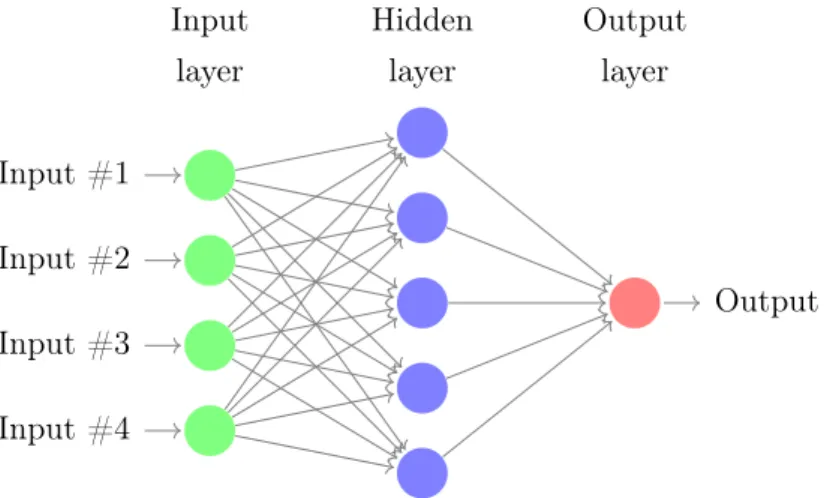
The architecture can be transformed to capture a more complex configuration of the inter-relation between multiple inputs and also their relationship with a single output. Figure 4.2 illustrates the case in which the structure of the neural network has one layer of multiple neurons between the input layer and output layer, i.e. hidden layer with more than one neuron.

Input #1 Input #2 Input #3 Input #4 Output Hidden layer Input layer Output layer

Figure 4.2: Neural Network with One Hidden Layer

The mathematical equivalent would be:

y = f (WX), (4.2)

where W and where X represent the weight and input matrices respectively. The weights wij are

(26)

4.1 Neural Networks 23 hidden layer and the number of hidden layers mainly depend on the complexity of the problem and nature of the data (Kabir & Ahsan Akhtar Hasin, 2013).

Some problems might require to deliver n diﬀerent regression outputs starting from an input vector of cardinality m. In other words, we will need to transform an m-dimensional input space into an n-dimensional output space:

Rm >Rn, (4.3)

Figure 4.3 illustrates a neural network with 4 input neurons, one single hidden layer with 5 neurons and 3 output neurons.

Input Layer Hidden Layer Output Layer

Figure 4.3: Multiple Output Neural Network with One Hidden Layer

In this case, the generic output yk will be the result of (Bishop, 1995):

yk= ˜f _Xt j=1 kjf ✓_Xm i=1 wjixi ◆ , (4.4)

with wji as the weight between input i and hidden neuron j and kj as the weight between

hidden neuron j and the output neuron k.

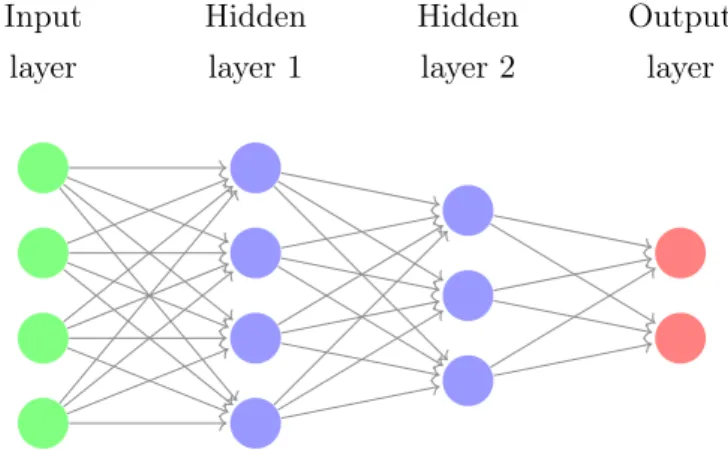
For MLPs (see Figure 4.4) back-propagation is the most notable learning rule (Le Cun, 1986; Parker, 1985). This technique propagates backwards the errors of the output neurons to the hidden neurons. This is particularly useful when the correct solution for the neurons is unknown, therefore we cannot directly calculate the error.

The back-propagation method is defined in two steps: one forward step and one backward step. Within the forward step, the outputs of the network are calculated propagating the inputs through the neurons of the network, while the weights of the connections remain unchanged. The backward step consists of a two sided modification of the weights of each connection as follows:

• For the output neurons, the weights will be modified through the Delta Rule. More specifi-cally, the weights of the connection between the last hidden layer and the network’s output layer will be iteratively re-calibrated by comparing the calculated output with the desired output and generating an error through an error function, e.g, mean squared error. The

(27)

pro-4.1 Neural Networks 24 cess will terminate when the error function will be lower than a predefined value (Widrow & Hoﬀ, 1960).

• For the hidden neurons, the remaining weights will be re-determined by propagating back-wards the above-mentioned error assuming that the error attributed to one neuron is the sum all errors in all subsequent directly connected neurons.

The weight between a generic neuron i and a generic neuron j are at each stage updated through:

wij = wij + wij, (4.5)

with wij depending on the error function E:

wij = ⌘

@E @wij

. (4.6)

The above equation implies that the algorithm moves towards a solution by means of the gradient descent method where a specified learning rate, ⌘, is employed as movement length (Ranganathan, Nakai, & Schonbach, 2018). In practical terms, the weights are continuously modified in the negative direction of the gradient of the error. The algorithm will stop and the weights will no longer be modified when the minimum of the error function is reached, i. e. the derivative of E is zero. Input layer Hidden layer 1 Hidden layer 2 Output layer

(28)

4.1 Neural Networks 25 4.1.1 Recursive Neural Networks

x(t 2) w2

f

x(t + 1)ˆ Output x(t) Inputs w1 x(t 3) w3 Weights

Figure 4.5: Single Neuron Perceptron with Time Dependent Input Data

The ANN results inadequate to forecast time sequential data sets, where each element in the input vector will depend on the time it was measured, as illustrated in Figure 4.5. This means that the input at time t will have a certain dependency to the input observed at time t 1. Up until now, we have examined neural networks where the information flows in one single direction, from the input to the output, i.e. feed forward neural networks. Still, it is possible to build neural networks where the information moves in one direction but also in the opposite direction generating loops which allows for information to persist. These are referred to as Recursive (or Ciclic) Neural Networks and were discovered by Hopfield (1982), Rumelhart, McClelland, and PDP Research Group (1986). Recursive neural networks result particularly eﬀective when dealing with time series, provided their ability to learn sequentially (Gamboa, 2017).

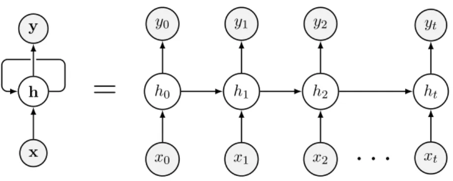
Figure 4.6 and Figure 4.7 illustrate the transition of information within the structure of a vanilla Recursive Neural Network and within a generic Recursive Neural Network architecture respectively. h0 h1 h2 ht

=

h y0 x0 y1 x1 y2 x2 yt xt y x

. . .

Figure 4.6: Unfolded Recurrent Neural Network with one input, one output, one hidden layer and one recurrent layer

In the above figure, a network h captures the information from a sequential input x and generates an output y. The network h consists of a collection of states {h0, h1, h2, . . . , ht}. These initially

(29)

4.1 Neural Networks 26 read each input incrementally and subsequently the network constantly loops all over again while keeping memory of all the processed information.

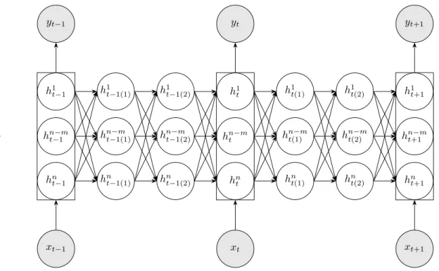
Each state h can contain different neurons within different layers. Figure 4.7 shows an example of Recursive Neural Network (RNN) where all states hold three interconnected layers, each with ndifferent neurons. Moreover, the final layer of a certain state at time t will be connected with the first layer of the subsequent state at time t + 1.

h1 t 1 hn mt 1 hn t 1 yt 1 xt 1 h1 t 1(1) hn m_{t 1(1)} hn_{t 1(1)} h1 t 1(2) hn m_{t 1(2)} hn_{t 1(2)} h1 t hn mt hn t yt xt h1 t(1) hn m_t(1) hn_t(1) h1 t(2) hn m_t(2) hn_t(2) h1 t+1 hn mt+1 hn t+1 yt+1 xt+1 . . . .

Figure 4.7: Unfold Recurrent Neural Network with multiple inputs, outputs and layers

The output at current time step, yt, of a vanilla RNN, provided the input at current time step,

xt, and the hidden state, h, at time step t 1, can be defined as (Finsveen, 2018):

yt= f (L[xt, ht 1]), (4.7)

L[xt, ht 1] = W1xt+ W2ht 1+ ✏. (4.8)

Where L is a linear transformation function, f is typically a non-linear function, W1 and W2

are weight matrices and ✏ is the remaining bias.

While for a MLP RNN dynamic, given layer l and time t, the state transition from the previous to the current neuron can be defined as a function (Zaremba, Sutskever, & Vinyals, 2014):

RN N : hl 1_t , hl_{t 1}_{! h}l_t, (4.9) with:

hl_t= f (L[hl 1_t , hl_{t 1}]). (4.10) 4.1.2 Long-Short Term Memory Neural Networks

One problem that frequently arises when using RNN for time series forecasting is their "for-getfulness". They are unable to record long term dependencies and typically retain unnecessary

(30)

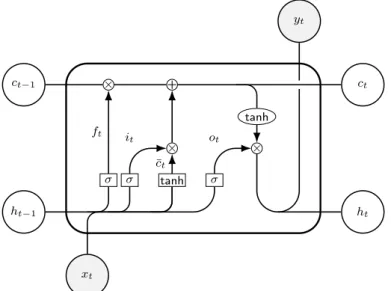
4.1 Neural Networks 27 information (Bengio, Simard, & Frasconi, 1994; Petneházi, 2018). A variant of RNN, the Long Short Term Memory (LSTM) network, was introduced by Hochreiter and Schmidhuber (1997) to memorize long term patterns when necessary, recall what it needs to be recalled and learn only what needs to be learned.

A LSTM layer can be composed by one or more LSTM units. Within each unit the LSTM struc-ture consists of a new hidden state that will act as the memory of the networks, i.e. cell. The memory of the cell can be altered through a single neural network layer called gate. The weights of these networks need to be learned during the training phase.

The gates of a LSTM will enable the process of retaining the necessary memory from the current input, forgetting unnecessary patterns and generating a current output based on the present and past memory. Each LSTM unit will receive three inputs: the previous short term output, the long term memory cell state generated by the previous unit and the current input. Subsequently the forget gate, output gate and input gate along with additional gates that perform regularisa-tion will process the informaregularisa-tion and deliver a long term memory cell and a short term memory output.

Formalizing, an LSTM unit receives at a generic time t a cell ct 1 and the short term memory

output ht 1 from the previous LSTM unit and the current input xt. Provided the parameters

W1, W2 and ✏f, the forget gate will generate an output ft through the sigmoid function, :

ft= (W1,fxt+ W2,fht 1+ ✏f), (4.11)

and this defines the unnecessary memory to be erased (Goel, Melnyk, Oza, Matthews, & Banerjee, 2016).

At this point we can determine what memory needs to be added to the new cell state ct as

follows:

it= (W1,ixt+ W2,iht 1+ ✏i), (4.12)

¯

ct= tanh(W1,cxt+ W2,cht 1+ ✏c), (4.13)

ct= it c¯t+ ft ct 1, (4.14)

where is the Hadamard element-wise product and ¯ctrepresents a candidate state.

The last missing element is the output of the cell state at time t, ht, which can also take the

form of the final output of the LSTM structure, yt. This is defined through the output gate as

below:

ot= (W1,oxt+ W2,oht 1+ ✏o), (4.15)

ht= ot tanh(ct 1). (4.16)

(31)

4.1 Neural Networks 28 tanh ⇥ + ⇥ ⇥ tanh ct 1 ht 1 xt ct ht yt ft _i_t ¯ ct ot

Figure 4.8: LSTM unit diagram

4.1.3 Monte Carlo Dropout

The typical actuarial modus operandi implies predictive uncertainty estimates. In deep learning there is no clear way to determine Bayesian estimates. Gal and Ghahramani (2016) proposed to train a model with a variational dropout method to extract Monte Carlo samples. This will allow for inference on the posterior distribution of the neural network weights provided a prior distribution of the weights.

Given Bayesian theory, we can determine a posterior probability of an observed vector of weights of a generic neural network, !, given data X, as (Shahroudi, 2019):

p(!_{|X) =} p(!|X)p(!)

p(X) , (4.17)

where p(!|X) is the probability of X conditional to the current weights, p(!) is the prior distri-bution of the weights and p(X) is the probability related to the input data.

The probability of observing one single point, ¯x, provided all inputs and parameters of the model can be determined through:

p(¯x|X, !) = Z

p(X|!)p(!|X)d!. (4.18)

Let X and Y be two separate data sets, the prediction of a point ¯y given a new data point ¯x will be determined as below:

p(¯y|¯x, X, Y, !) = Z

p(¯y, ¯x|!)p(!|X, Y)d!. (4.19) Typically, the prior distribution of the weights is assumed to be distributed as a standard normal random variable for each layer and the bias vector is presumed to take the form of a point estimate.

The dropout (at training time) is a process that randomly ignores neurons within a specified set and it generally serves as a regularisation tool to prevent over-fitting. However, Gal and

(32)

4.2 Termination Risk 29 Ghahramani (2016) performed a dropout process in the form of variational inference, i.e. at test time, to approximate the prediction. Consequently, the predictions at test time will no longer be deterministic. But, the output will depend on which neurons were ignored. Thus, by performing dropout at test time and assuming a Normal distribution for the weights, we can approximate p(¯y_{|¯x, X, Y, !) as an average of the results, i.e. Monte Carlo Dropout (MCD):}

p(¯y|¯x, X, Y, !) ⇡ 1 T T X t=1 p(¯y|¯x, ˆ!t), (4.20)

where ˆ!t represents the estimated weight vector.

4.2 Termination Risk

Termination Risk is a risk related to the uncertainty of the PVI contract term. Diﬀerent situa-tions might cause unexpected termination, e.g. downsizing, refinancing and significant intentional damage to the property.

However, this product has been designed to finance old age income streams and thus to cease upon death of both signatory spouses. For such reason and provided the available information, we will consider longevity risk as the sole termination risk driver. This will require a model to fit and predict mortality. A particular stochastic technique has been dominating mortality mod-elling: the Lee Carter Mortality Model (LCMM) (R. D. Lee & Carter, 1992). This will be used to determine Italian mortality components.

The necessary input mortality data for the Italian population is retrieved form the Human Mor-tality Database (2019). Additionally, we will adopt and expand the model through the LSTM approach developed by Richman and Wüthrich (2018), Nigri, Levantesi, Marino, Scognamiglio, and Perla (2019). The framework will be employed to forecast the time dependent parameter of the LCMM. All these methodologies will be again expanded by adding MCD.

4.2.1 The Lee Carter Mortality Model

The LCMM is the current mortality forecasting standard model. It designs a structure for the central mortality rate, mx,t. This is the proportion of deaths on the exposed to death recorded for

age x during year t. Its architecture was derived from averaging log mortality rates and applying Support Vector Decomposition (SVD) to the residuals to achieve the following form:

log(mx,t) = ↵x+ xkt+ ✏x,t, (4.21)

where ↵x, ktand x are the parameters of the model which can be interpreted as the logarithm

of the geometric mean of empirical mortality rates, the time trend of mortality and the age-specific mortality deviations from the overall trend, respectively. Whereas, ✏x,t represents the

random eﬀects of age and time which in traditional time series models is formulated as a series of independent normally distributed random variables.

Additionally, to achieve unique solutions the following constraints are necessary: X

x

b2_x= 1 and X

t

(33)

4.2 Termination Risk 30 R. D. Lee and Carter (1992) estimate parameters ↵x, xand ktthrough a two stage least square

error approach. First ↵x was estimated as:

ˆ ↵ = 1 T T X i=1 log(mx,t) (4.23)

and ˆx and ˆkt were computed through a singular value decomposition of matrix [log(mx,t) ↵ˆx].

If used alone, this procedure doesn’t guarantee that the observed number of deaths equals the fitted number of deaths. Hence, a second estimation stage was introduced to fit kt such that:

dt=

X

x

exp_{(↵x+ xkt)⇥ Ex,t}, (4.24)

where dt is the number of deaths at time t and Ex,t is the population of age x exposed to death

at time t.

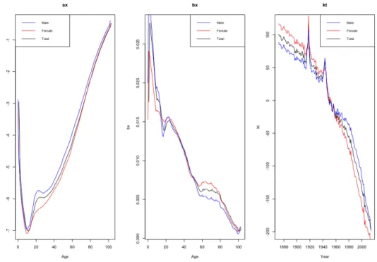
The estimates of ↵x, x and kt using LCMM with the two-step procedure on yearly Italian

mortality rates observed between 1872 and 2014 for ages between 0 and 110 are illustrated in Figure 4.9.

Figure 4.9: LCMM parameter estimates

The estimated kt will serve as time series base for the forecasting technique outlined in the

following section.

4.2.2 Single-Output LSTM Modelling

Provided the above theoretical framework, we’ve created a MCD LSTM model to forecast future values of ktand consequently mortality rates separated by male, female and total population. To

this end, first the univariate LSTM parameters have been calibrated with a number of neurons and training epochs depending on the gender modelled. The data set has been divided into an

(34)

4.2 Termination Risk 31 80% training set and a 20% test or validation set. These two data sets were used to tune all hyper-parameters of the model, i.e. number of layers, number of neurons per layer and tuning epochs.

For this purpose, the error in terms of a pre-defined loss function produced by the LSTM model applied to the training set has been compared with the validation set error function. This al-lowed for over and under-fitting diagnosis. A higher loss function originating from the test set is typically characteristic of an under-fitted model. While, a lower test set loss function is symptom of an over-fitted network.

The validation set’s error path would indicate whether capacity could be improved by re-calibrating neurons, hidden layers or training epochs. As such, when the validation set would produce a flat higher error amount, the number of hidden layers and/or neurons were increase. Alternatively, if the error function would present a lower value than the training set and a flat tendency, this would suggest an under-fitting diagnosis which could be improved by reducing hidden layers and/or neurons. If the error trend was decreasing for higher test set loss amounts or increasing for lower error values, the number of training periods would need to be raised1_.

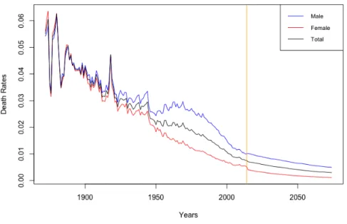
Subsequently, we’ve generated 1000 random simulations using MCD modelling for the first future steps. These random simulations were used to generate each one path for 60 time steps which were then used in formula 4.21 to generate 1000 simulations for mortality rates for a given age. From these we’ve extracted the average value which would ultimately define the final prediction for the next 60 years. Figure 4.10 displays mortality for the input dates along with the predicted mortality for a population aged 65.

Figure 4.10: Mortality predictions for a population aged 65.

While the 1000 future mortality simulations are shown in Figure 4.11 separately by female and male population.

(35)

4.3 Financial Risk 32

Figure 4.11: Mortality simulations for females and males both aged 65 displayed on the left side and on the right side respectively.

4.3 Financial Risk

Along with termination risk any RM contract presents a second class of risks: Financial Risks. These originate from the uncertainty within interest rates, mortgage rates and property appre-ciation or depreappre-ciation rates and, when the annuity is indexed to prices, i.e. inflation rates. It has been proven that all these variables are correlated (Alai et al., 2014; D. W. Cho et al., 2013). In a VAR perspective that generates stochastic scenarios, these variables would be mod-elled together to take advantage of the their correlation when predicting future values. The VAR analysis would typically include also Gross Domestic Product (GDP) in the modelling phase to generate a more accurate prediction, provided its high correlation with the above-mentioned variables. Thus, we will employ all these variables to produce our financial risk model.

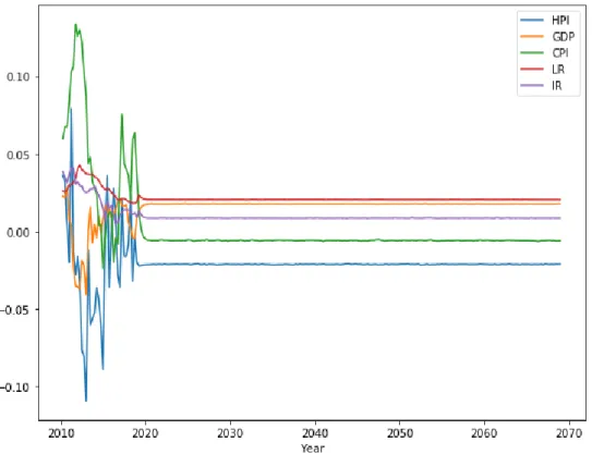
However, Verstyuk (2018) has shown that an LSTM approach outperforms the VAR technique when modelling economic variables. Therefore, a MCD LSTM perspective appears more suitable for our risk assessment problem.

The economic data set used to estimate the parameters of the predictive model is composed by: 1. House Price Index (HPI), quarter availability between Q2 2010 and Q1 2019 (ISTAT,

2019b);

2. Euro Area Interest Rate (IR) with maturity 30 years, daily availability between September 6, 2004 and June 20, 2019 (European Cntral Bank, 2019);

3. Consumer Price Index (CPI) for the entire Italian territory and products, monthly avail-ability between January 1997 and June 2019 (ISTAT, 2019a);

4. GDP variation, annual availability between 2002 and 2019 (ISTAT, 2019c);

5. Loan Rate (LR), monthly availability between January 1995 and April 2019 (Banca d’Italia, 2019).

Provided the availability of HPI, the input data consists of quarterly variables for the periods between Q2 2010 and Q1 2019. Additionally, for homogeneity purposes the HPI, CPI and GDP