Joana Rafael Matzen
Neves da Silva
BIODIVERSIDADE E EVOLUÇÃO MOLECULAR DA
CLASSE MALACOSTRACA
BIODIVERSITY AND MOLECULAR EVOLUTION OF
MALACOSTRACA
Joana Rafael Matzen
Neves da Silva
BIODIVERSIDADE E EVOLUÇÃO MOLECULAR DA
CLASSE MALACOSTRACA
BIODIVERSITY AND MOLECULAR EVOLUTION OF
MALACOSTRACA
Dissertação apresentada à Universidade de Aveiro para cumprimento dos requisitos necessários à obtenção do grau de Doutor em Biologia, realizada sob a orientação científica da Professora Doutora Maria Marina Ribeiro Pais da Cunha, Professora Auxiliar do Departamento de Biologia da Universidade de Aveiro, Doutor Filipe José Oliveira Costa, Professor Auxiliar da
Universidade do Minho e do Professor Doutor Gary Robert Carvalho, Professor do Departamento de Biologia da Universidade de Bangor, País de Gales, Reino Unido.
Joana Matzen da Silva was supported by a PhD grant (SFRH/BD/25568/ 2005) from Fundação para a Ciência e Tecnologia, co-funded by POCI/FSE,
and projects Hermes (FP6 EC – GOCE-CT-2005-511234), Hermione (FP7 EC – 226354) and LusoMarBol (FCT – PTDC/MAR/69892/2006).
It seems to me that the natural world is the greatest source of excitement; the greatest source of visual beauty; the greatest source of intellectual interest. It is the greatest source of so much in life that makes life worth living.
David Attenborough
To my greatest source of love, my parents Gisela and Rafael; the greatest source of friendship, my sisters Püppi and Catarina; and the greatest source of strength, my grandmothers Ilse and Irene.
o júri
presidente Professor Doutor António Carlos Mendes de Sousa Professor Catedrático da Universidade de Aveiro
Professor Doutor Amadeu Mortágua Velho da Maia Soares Professor Catedrático da Universidade de Aveiro
Professor Doutor Gary Robert Carvalho (Coorientador)
Professor of Molecular Ecology, University of Bangor, School of Biological Sciences, University of Wales, Bangor
Professor Doutora Maria Manuela Gomes Coelho Noronha Trancosa Professora Associada da Faculdade de Ciências da Universidade de Lisboa
Professor Doutor Henrique José de Barros Brito Queiroga Professor Auxiliar da Universidade de Aveiro
Doutor Filipe José Oliveira Costa (Coorientador)
Professor Auxiliar da Escola de Ciência da Universidade do Minho
Professora Doutora Maria Marina Ribeira da Cunha (Orientadora) Professora Auxiliar da Universidade de Aveiro
Professor Doutor Simon Creer
Senior Research Fellow, University of Bangor, School of Biological Sciences, University of Wales, Bangor
Professor Doutor Ricardo Jorge Guerra Calado
Investigador Auxiliar do CESAM – Centro de Estudos do Ambiente e do Mar da Universidade de
agradecimentos I would like to acknowledge my supervisors Marina Cunha, Filipe Costa and Gary Carvalho for all the guidance and support given during these years. They gave me the opportunity to join there labs, where I had the chance to expand my scientific horizons and grow as a biologist. Additionally, Simon Creer has provided support throughout the project, for which I acknowledge his guidance, encouragement, optimism and numerous suggestions.
I have the happiness to come a cross with such fantastic people that have contributed in one way or another for this work:
- By providing biological material: Marina Cunha from Aveiro University, Antonina dos Santos from IPIMAR, Niklas Tysklind; Sarah Helyar and Ashley Tweedale from Bangor University; Jim Drewery from Aberdeen Fisheries Research Services from Scotia; Debbie Bailie from Queens University; Marco Arculeo from University of Palermo; Pere Abello from “Institut de Ciències del Mar (CSIC)” from Barcelona, Mark Dimech from Malta University; Joao Brum from Azores University; Luis Rodrigues, Manuel Baixio and Domingos Vieira from “Associação Marítima Açoreana” and to all fishermen from the vessels “Coração do Oceano” and “Mestre Domingos” from Azores (São Miguel island). - By helping me with morphological identification: Antonina dos Santos from IPIMAR, Simon Webster from Bangor University, Maria Włodarska-Kowalczuk from Institute of Oceanology PAS from Sopot, and Marco Arculeo from
University of Palermo. Judite Alves and Alexandra Cartaxana for archiving and being responsible for the Crustacean collection in the Natural and History Museum of Portugal.
- By helping me with DNA and phylogenetic analyses: Simon Creer, Markos Alexandrou, and Axel Barlow from Bangor University. Wendy Grail from Bangor University to help me with all lab equipment that was essential to my work. And finally I want to express a enormous gratitude to my work colleagues and friends: Jan Albin, Niklas Tysklind, Gregg Aschroft, Lou and Nick Dawnay, Sónia Pascoal, Markos Alexandrou, Axel Barlow, Edson Sandoval, Jacqui Eales, Serinde Van Wijk, Muni, Wendy Grail, Julia Gomes, Yolanda Higueras, Fraibet Aveledo, Vivi Fournière, Hanna Pavlickova, José António Matos, Fernanda Simões, and Antonina dos Santos, that always were supportive in difficult moments and were proud of happy and success “sampling” moments stored along this years.
A special thank you to my “God sister” Ana Elisabete Pires who has always been an excellent professional advisor and good friend for the past 10 years. To my family who I love unconditionally, thousand times thank you!
palavras-chave Malacostraca, Decapoda, Amfipoda, Isopoda, ADN código de barras, biodiversidade, filogenia, COI, 16S, 28S, numts
resumo No actual cenário de perda acelerada de biodiversidade, o nosso conhecimento dos ecossistemas marinhos, apesar da sua extensão e
complexidade, continua muito inferior ao dos ecossistemas terrestres. A classe Malacostraca (Arthropoda, Crustacea), um grupo dos mais representativos nos ecossistemas marinhos, apresenta um elevado nível de diversidade
morfológica e ecológica, mas difícil sua identificação ao nível de espécie requer frequentemente a ajuda de especialistas em taxonomia. A utilização recente do “barcoding” (código de barras do ADN), revelou ser um método rápido e eficaz para a identificação de espécies em diversos grupos de metazoários, incluindo os Malacostraca. No âmbito desta tese foi construída uma base de dados de código de barras de ADN envolvendo 132 espécies de Malacostraca vários locais de amostragem no Atlântico Nordeste e
Mediterrâneo. As sequências de ADN mitocondrial provenientes de 601 espécimes formaram, em 95% dos casos, grupos congruentes com as identificações baseadas em características morfológicas. No entanto, foi detectado polimorfismo em seis casos e a divergência intra-específica foi elevada em exemplares pertencentes a duas espécies morfológicas, sugerindo, neste caso, a ocorrência de especiação críptica. Este estudo confirma a utilidade do código de barras de ADN para a identificação de Malacostraca marinhos. Apesar do sucesso obtido, este método apresenta alguns problemas, como por exemplo a possível amplificação de
pseudogenes. A ocorrência de pseudogenes e as possíveisabordagens para a detecção e resolução deste tipo de problemas são discutidas com base em casos de estudo: análises dos códigos de barras ADN na espécie Goneplax
rhomboides (Crustacea, Decapoda). A análise dos códigos de barras ADN
revelou ainda grupos prioritários de decápodes para estudos taxonómicos e sistemáticos, nomeadamente os decápodes dos géneros Plesionika e
Pagurus. Neste âmbito são discutidas as relações filogenéticas entre espécies
seleccionadas dos géneros Plesionika e Pagurus.
Este trabalho aponta para várias questões no âmbito da biodiversidade e evolução molecular da classe Malacostraca que carecem de um maior esclarecimento, podendo ser considerado como a base para estudo futuros. Análises filogenéticas adicionais integrando dados morfológicos e moleculares de um maior número de espécies e de famílias deverão certamente conduzir a uma melhor avaliação da biodiversidade e da evolução dentro da classe.
keywords Malacostraca, Decapoda, Amphipoda, Isopoda, DNA barcode, biodiversity, phylogeny, COI, 16S, 28S, numts
abstract The biodiversity of many habitats is under threat and although seas cover the majority of our planet’s surface, far less is known about the biodiversity of marine environments than that of terrestrial systems. The complexity of its species and ecosystems is immense.
Marine malacostraca are known as a group with a high level of morphological and ecological diversity but are difficult to identify by traditional approaches and usually require the help of highly trained taxonomists. A faster identification method, DNA barcoding, was found to be an effective tool for species identification in many metazoan groups including some malacostraca. Moreover, the generation of a larger comparative database allows additional insights into the tempo and mode of molecular evolution. Indeed, examination of diversity at the COI region yields an informative framework to identify and explore priority issues, demanding in turn a fully integrative approach utilising additional molecular, distributional and ecological information. Here we expand the DNA barcode database with a case study involving more than 132
malacostracan species from the Northeast Atlantic Ocean and Mediterranean Sea. DNA sequences from around 601 specimens grouped into clusters corresponding to known morphological species in 95% of cases. However shared polymorphism between sister-species was detected in six species. Intraspecific divergence was high in specimens belonging to two morphological species, suggesting the occurrence of cryptic speciation, allowing a rapid assessment of taxon diversity in groups that have until now received limited morphological and systematic examination. We highlight taxonomic groups or species with unusual nucleotide composition or evolutionary rates. Such data are relevant to strategies for conservation of existing decapod biodiversity, as well as elucidating the mechanisms and constraints shaping the patterns observed.This study reconfirms the usefulness of DNA barcoding for the identification of marine malacostraca, despite complexities that sometimes arise due to pseudogenes (numts). Here, we study the effect of numts on DNA barcoding based on barcoding analyses in decapoda species: Goneplax
rhomboides. DNA barcodes reveal priority groups for taxonomic and systematic
focus of decapods. Here we discussed two cases of phylogenetic relationships among selected species of Plesionika and Pagurus, respectively.
Issues relating to the molecular biodiversity and evolution of the Malacostraca arising from this study allow identification of future priorities. Further
phylogenetic analyses including morphological and molecular data of selected families is required, especially encompassing broad geographic and ecological coverage, will lead to an improved evaluation of the biodiversity and evolution among selected Malacostraca species.
LIST OF FIGURES
vLIST OF TABLES
xi
SECTION 1. GENERAL INTRODUCTION
1
1.1 Marine biodiversity and evolution 5 1.1.1 Biodiversity and its conservation 13 1.1.2 Biodiversity and evolution of marine Malacostraca 16 1.1.2.1 Synopsis: Malacostraca morphology 17 1.1.2.2 Synopsis: Malacostraca phylogeny 21 1.2 Concepts and the molecular methods used in this study 23
1.2.1 Molecular diversity 24
1.2.2 DNA sequencing 27
1.2.2.1 Mitochondrial genes 29
1.2.2.2 Nuclear genes 33
1.2.3 Phylogenetic inference methods 35 1.2.3.1 Models of DNA sequence 35 1.2.3.2 Assessing node confidence in phylogenetic trees 40 1.3 Aim and output of the thesis 44
Reference 46
SECTION 2. MOLECULAR BIODIVERSITY
57
Chapter 2.1. DNA barcodes of Malacostraca species from the Northeast Atlantic
Ocean and Mediterranean Sea 61
Abstract 62
2.1.1 Introduction 63
2.1.2 Material and methods 75
2.1.3 Results 83 2.1.4 Discussion 90 2.1.5 Conclusions 100 Acknowledgments 103 References 104 2.1.6 Annex 117
Abstract 160
2.2.1 Introduction 161
2.2.2 Material and methods 168
2.2.3 Results 173 2.2.4 Discussion 181 2.2.5 Conclusions 184 Acknowledgments 185 References 185
SECTION 3. MOLECULAR EVOLUTION AND SHALLOW
PHYLOGENIES
189
Chapter 3.1. Systematic and evolutionary insights derived from mtDNA COI
barcode diversity in the Decapoda 93
Abstract 94
3.1.1 Introduction 196
3.1.2 Material and methods 201
3.1.3 Results 208 3.1.4 Discussion 216 3.1.5 Conclusions 230 Acknowledgments 231 References 231 3.1.6 Annex 249
Chapter 3.2. Testing the utility of partial COI and 16S sequences for phylogenetic estimates of selected Plesionika (Decapoda: Pandalidae) from the
Northeast Atlantic and Mediterranean Sea 355
Abstract 356
3.2.1 Introduction 358
3.2.2 Material and methods 361
3.2.3 Results 367 3.2.4 Discussion 375 3.2.5 Conclusions 383 Acknowledgments 384 References 385
Chapter 3.3. DNA barcodes of the hermit crab genus Pagurus Fabricius, 1775 (Decapoda, Anomura, Paguridae) of the North Atlantic and
Mediterranean Sea indicate priority species for molecular taxonomy
examination 397
3.3.4 Discussion 416 3.3.5 Conclusions 420 Acknowledgments 421 References 421
SECTION 4. FINAL REMARKS 429
4.1 Overview 433
4.1.1 Molecular biodiversity 434
4.1.2 Molecular evolution and shallow phylogenies 436
4.2 Future perspectives 439
v
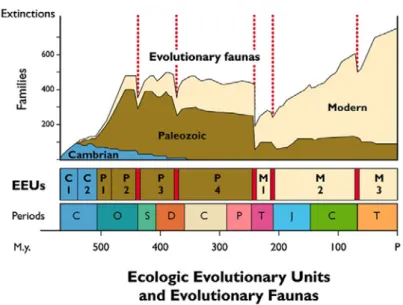
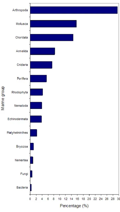
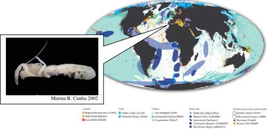
Figure 1.1: Family diversity of skeletonized marine invertebrates during the Phanerozoic (modified from Sheehan, 1996 in Harper 2006). The diagram includes evolutionary ecologic units (EEUs), together with an indication of the five large extinction events (red lines); and ten specified geological periods: Cambrian (C (blue)), Ordovician (O), Silurian (S), Devonian (D), Carboniferous (C (green)), Permian (P), Triassic (T (pink)), Jurassic (J), Cretaceous (C (green box)), Terciary (T (orange box)). 7 Figure 1.2: Contribution of each marine group (> 0.3%) for the total number of 150,891 (February 2010) valid species according to WoRMS (see Radulovici et al., 2010). 8 Figure 1.3: Average number of marine species described per taxon every year until 2010. Adapted from Radulovici et al., 2010. 12 Figure 1.4: A new species of ghost shrimp (Vulcanocalliax arutyunovi) found associated with mud volcanoes in the Gulf of Cadiz in the Northeast Atlantic is the second recorded thalassinidean crustacean from deep-sea chemoautotrophic communities (Dworschak and Cunha, 2007). Census of
Marine Life project areas map adapted from http://www.coml.org/ 15
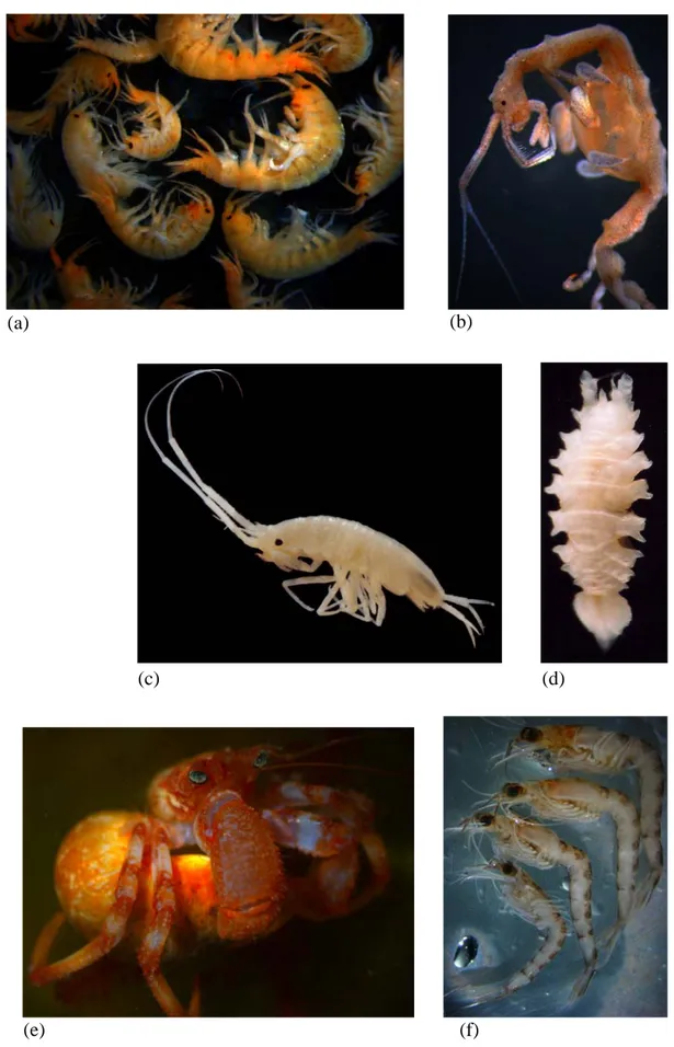
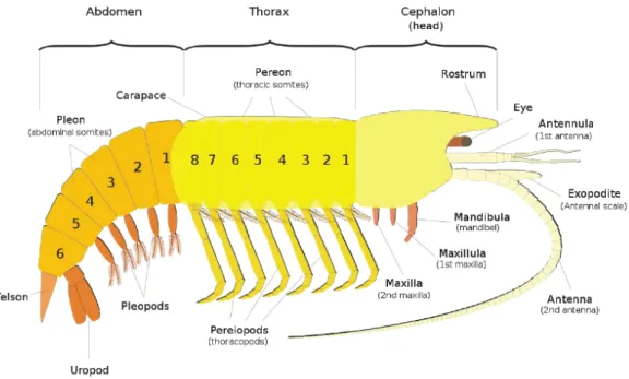
Figure 1.5: Eumalacostraca diversity. (a-b) Amphipoda; (c-d) Isopoda; (e) Decapoda; (f) Euphasiacea (photo credits J Matzen da Silva (a,b,d,e) and MR Cunha (c,d)). 19 Figure 1.6: General Malacostraca morphological characteristics: the head has 6 segments, with a pair of antennules and a pair of antennae, as well as mouthparts; stalked or sessile eyes; 8 pairs of thoracic legs, of which several pairs are often modified into feeding appendages, maxillipeds; 8 thoracic
segments; 6 abdominal segments (http://zipcodezoo.com/Key/Animalia/Malacostraca_Class.asp). 20
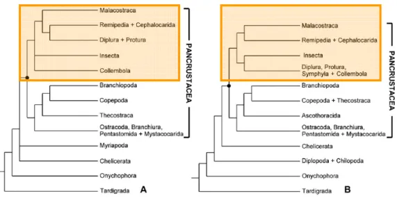
Figure 1.7: Arthropoda phylogenetic trees (A and B inferred by bayesian and likelihood analysis, respectively) based two mitochondrial markers, 16S rDNA and cytochrome c oxidase subunit I (COI), and the nuclear ribosomal gene 18S rDNA (adapted from Koenemann et al 2010). The variance positions of the Malacostraca sister groups is highlighted with orange boxes. In view of the methodological variations encompassed by Koenemann et al., (2010) study, it was unable to resolve the highest level relationships within Arthropoda due the limited number of species and molecular data. 21
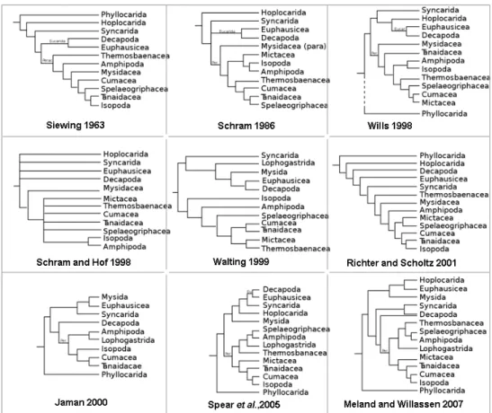
Figure 1.8: Malacostraca phylogenetic trees proposed by different studies. The first six trees were based on morphological characters whereas the last three were obtained with molecular data (adapted from Spears (Jarman et al., 2000; Meland and Willassen, 2007; Spears et al., 2005). E.g., look upon the evolution of the phylogenetic positions of two orders Amphipoda and Isopoda among all the 9 trees. 22
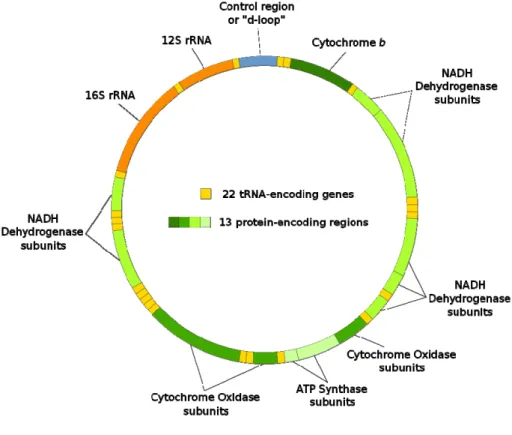
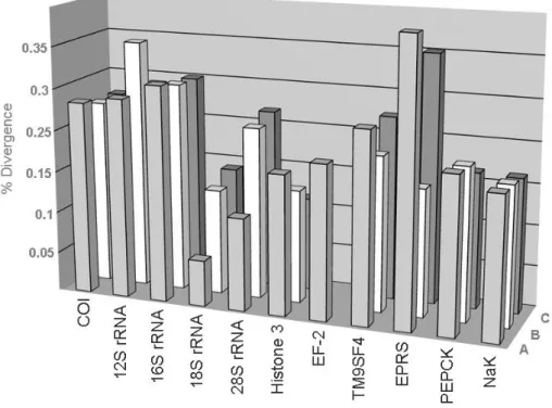
ribosomal RNA genes (12S and 16S), and a non-coding segment called the control region or “d-loop” (Harrison, 1989). 33 Figure 1.10:Pairwise nterspecific divergence among three different non congeneric decapods species pares (A; B; C) for mitochondrial (COI; 12S rRNA; 16S rRNA) and nuclear genes (18S rRNA; 28S rRNA; Histone 3; EF-2; Transmembrane 9 superfamily protein member 4 (TM9SF4); Glutamyl-prolyl-tRNA synthetase (EPRS); Transcriptional repression of the gluconeogenic (PEPCK); sodium– potassium ATPase o-subunit (NaK). Figure transformed from Toon et al., 2009. 35 Figure 2.1.1: DNA barcode analytical chain (figure provided personally by F.O. Costa adapted from P.D.N.Hebert). 75 Figure 2.1.2: Sampling sites of Malacostraca specimens from North East Atlantic Ocean and Mediterranean Sea (2001 to 2008). The ranges of specimens collected per species are represented by yellow (1 to 5), orange (5 to 50) and red balls (> 50), respectively. 82 Figure 2.1.3: Frequency distribution of intraspecific and interspecific COI barcode distances (K2P) from pairwise comparisons among members of the order Amphipoda, Decapoda and Isopoda (see Table 2.1.6). 86 Figure 2.1.4: Distribution of the genetic distances to the nearest-neighbour and mean intra-specific distance at COI sequences for 335 Malacostraca species compared. 89
Figure 2.1.5: Branches of the neighbour-joining tree (K2P model) highlighting the putative species complexes (and related species) found in decapods in this study. Bootstrap values based on 1000 replications are included. 89 Figure 2.2.1: Mechanism of numts insertion (figure adapted from Hazkani-Covo et al., 2010). Different mechanisms are here suggested: (A) The degradation of abnormal mitochondrial (Campbell and Thorsness, 1998). Mutant nuclear gene (yme1) have protein that are mitochondrial associated (Yme1p) and it has been suggested that perturbation in mitochondrial functions due to the alteration of gene products affect mitochondrial integrity by the vacuole, and this degradation increases mtDNA escape to nucleus in a process known as mitophagy and are more frequently than the wild-type strain (YME1); (B) lysis of mitochondrial comportment; (C) encapsulation of mitochondrial DNA inside the nucleus; (D) direct physical association between the mitochondria and the nucleus and membrane fusions; (E) MtDNA integrated into the chromosome during the repair of double strand breaks (DSBs) in a mechanism known as non-homologous end-joining (NHEJ). The insertion involves two DSB repair
vii
whole (see for review Hazkani-Covo et al. (2010)). 162 Figure 2.2.2: Numt content is correlated to genome size (adapted from Hazkani-Covo et al., 2010). 165 Figure 2.2.3: Photography took in this study of representative morphotype specimens G. rhomboides (G. romboides 01) collected from South Portuguese coast and sequenced twice with two different COI primers set COI-III and COLH (Table 2.2.1). 167 Figure 2.2.4: Eye and anterolateral border of the carapace: (A) Goneplax clevai n. sp and (B) G. rhomboides (Linnaeus, 1758) (photography adapted from Guinot and Castro 2007). 167
Figure 2.2.5: Steps to help avoid and identify numts contamination in DNA barcoding (figure modified from Song et al. 2008). A new step is proposed in this study to be added on the previous protocol when the chromatogram examinations pass to the quality control. 171
Figure 2.2.6: Screenshot example of 5´COI sequences, translation and chromatograms from our representative G. rhomboides 01 COLH and five questionable COI sequences amplified with M13- tailed cocktail primers (COI-III). The variety of colours along the sequence text, each colour represents a different amino acid translated along 564 bp of COI sequence. No stop codons and indels have prevented translation in our data set. 174
Figure 2.2.7: Radiation tree (BI) of representatives from 20 G. rhomboides (01 to 20) amplified with different primer set (see Table 2.2.1: Folmer; CrustD; COLH; COI-III). Posterior probabilistic BI values > 75% are represented in each node of the tree. Orange baloon are selected the questionable numts sequences and in gray baloon the orthologous COI sequences. 177 Figure 2.2.8: Amino acid variation among five questionable numts (G. rhom 01 to 05 COI-III), one representative of our COI sequences (G. rhom 01 COLH) and NC_06891 as orthologous COI reference. Positions with amino acid variations are marked with bars. Symbol ” * “highlight variation between NC_06891 and the reference G. rhom 01 COLH. 180 Figure 3.1.1: Intraspecific diversity assessment: the effect of sampling bias, non-monophyletic clades, putative cryptic species and congeneric species with low genetic distance. Solid lines represent the raw
data for the total data set (AR, black lines) and for the dataset in which non-monophyletic clades,
putative cryptic species and congeneric species with low genetic distance were removed (BR, blue
lines). The dashed lines represent results for the data in which all taxa have the same weight (mean
Figure 3.1.3: Boxplot distribution of 11 selected families of the Decapoda order intraspecies (S), intragenus (G), and intrafamily (F) COI K2P distances (%). The plot summarises median (central bar), position of the upper and lower quartiles (called Q1 and Q3, central box), extremes of the data (dots) and very extreme points of the distribution that can be considered as outliers (stars). Points are considered as outliers when they exceed Q3 + 1.5(Q3-Q1) for the lower part, where (Q3-Q1) is the inter quartile range. The number of sequences, species, and genera per family are given in Table 3.1.3. Mean K2P distance (%) ± SE within taxa are: Chirostylidae S=0.701 ± 0.028 and G=8.999 ± 0.039; Lithodidae S=0.416 ± 0.021, G=6.376 ± 0.137 and F=11.392 ± 0.063; Paguridae S=0.686 ± 0.045 and G=17.173 ± 0.084; Parastacidae S=1.375 ± 0.131, G=11.017 ± 0.078 and F=22.681 ± 0.064; Majidae S=0.547 ± 0.028, G=9.643 ± 0.214 and F=21.084 ± 0.061; Portunidae S=0.453 ± 0.024, G=14.826 ± 0.311 and F=28.929 ± 0.047; Galatheidae S=0.285 ± 0.017, G=16.839 ± 0.04 and F=22.355 ± 0.033; Atyidae S=0.758 ± 0.041, G=13.475 ± 0.352 and F=25.218 ± 0.056; Pandalidae S=0.49 ± 0.042, G=20.924 ± 0.213 and F=25.617 ± 0.07; Palaemonidae S=0.812 ± 0.055, G=20.157 ± 0.108 and F=25.398 ± 0.048; Crangonidae S=0.344, G=19.991 ± 0.514 and F=25.241 ± 0.103. 212 Figure 3.1.4: Boxplot distribution of ascending GC content (%) from 11 selected families. The number of sequences, species, and genera per family is indicated in Table 3.1.3 and statistic values in Table 3.1.4. 214 Figure 3.2.1: Pandalidae shrimps sampling locations from our study (see Table 3.2.1). 362 Figure 3.2.2: Bayesian phylogeny analyses of Pandalidae species for COI gene. A similar tree topology was obtained by Maximum likelihood (ML).The small numerals represent levels of support based on 500 bootstrap replicates /Bayesian Posterior Probabilities (ML/BI) expressed as percent. Values <50% are not show. Right braces indicate two groups: group A represent species with preference of subtropical and temperate zones and group B with preference of temperate and frigid zones. The black star indicates deep sea species samples from North Hemisphere and grey star species samples from South Hemisphere from Indic Pacific oceans. 371
Figure 3.2.3: Bayesian phylogeny analyses of 21 Pandalidae from the combined COI and 16S data. A similar tree topology was obtained by Maximum likelihood (ML).The small numerals represent levels of support based on 500 bootstrap replicates /Bayesian Posterior Probabilities (ML/BI) expressed as percent (values below the nodes represent levels of support only for COI). Right braces indicate two groups: group A represent species with preference of subtropical and temperate zones and group B with preference of temperate and frigid zones. The black star indicates deep sea species samples from North Hemisphere and grey star species samples from South Hemisphere from Indic Pacific oceans. 373
ix
Northwest Atlantic Ocean (NWA), North Atlantic Ocean (NA), Mediterranean Sea (MED) and Bering Sea (BER) (see Table 3.2.3 for complement information).Two major clades have been roman number-coded, I and II: represent two groups defined previously by Ingel (1985) based on adult and larvae morphological characters. 411 Figure 3.3.2: BI phylograms of each individual gene (COI, 16S, 28S) and concatenated data set (CON= COI+16S+28S). The numbers on branches are posterior probabilities >50% of BI (in percentage). Species P. alatus and P.excavatus are highlighter a bold. 413
xi
Table 1.1: List of major higher taxonomic groups of marine, freshwater and terrestrial flora and fauna. Modified from Roff and Zacharias, 2011. 9 Table 1.2: Species concepts and their strengths and weaknesses (Claridge et al., 1997; Gosling, 1994). 10
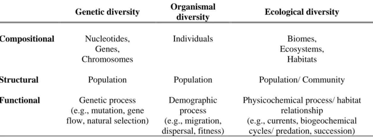
Table 1.3: Compositional, structural and functional attributes of biodiversity for marine environments
(Gaston and Spicer, 2009; Roff and Zacharias, 2010). 12
Table 1.4: Class Malacostraca down to the Order level, according to Martin and Davis (2001). Figures
modified from Barnes et al., 1996. 18
Table 1.5: A comparison of DNA-based species identification techniques. Modified from Wong and
Hanner (2008). 26
Table 1.6: Comparison of phylogenetic inference methods. Modified from Holder and Lewis (2003)
and Hall (2008). 40
Table 1.7: Tree construction and tree searching methods. Adapted from Holder and Lewis (2003). 41 Table 2.1.1: Bioinformatics of DNA barcoding: examples of methods used in DNA barcode analyses and ways to present the results. Modified from Casiraghi et al., 2010. 69 Table 2.1.2: Some users of taxonomic information and their potential interest in DNA-based
identification (adapted from Hollingsworth, 2007). 73
Table 2.1.3: DNA barcoding projects designed in this study under two campaigns of Barcode of Life Database. 78 Table 2.1.4: PCR primer sets or cocktails used to amplify COI. M13 tails are in italic when present. 80 Table 2.1.5: List of sequences retrieved from GenBank displaying conflicting species assignments or unusually high intraspecific divergences when compared against other published mitochondrial barcodes. 84 Table 2.1.6: Summary of the genetic divergences (K2P) for increasing taxonomic levels. Data are from 902 sequences from 335 species, 202 genera, 101 families and three orders. 88
132 species analysed to the nearest-neighbour at COI (K2P distance). 92 Tabel 2.2.1: Selected G. rhomboides with respective sample name, museum catalogue number, site of collection, COI primer set tested and genetic database accession numbers (Genbank). 170 Table 2.2.2: Pairwise COI barcode nucleotide divergences for G. rhomboides using K2P distances (%). 178
Table 2.2.3: Nucleotide diversity composition founded in 30 positions among 564 bp of 25 sequences of G. rhomboides. 179 Table 3.1.1: Combined data set derived from new data generated herein and publicly available DNA
barcoding projects from the Barcode of Life Database. 201
Table 3.1.2: Pairwise COI barcode nucleotide divergences for the Decapoda using K2P distances (%). 211
Table 3.1.3: Number of Decapoda sequences, species, genera and families analyzed in the present
study. 213
Table 3.1.4: Variation of GC content in the COI barcode region and codon position among the
Decapoda and from 11 selected families. 213
Table 3.2.1: Pandalidae shrimps used for the Plesionika phylogeny reconstruction and outgroup taxa. 360
Table 3.2.2: Nucleotide ML distances estimated from 16S with TrN+G model (above diagonal) and COI (below diagonal) with GTR+G+I model in Pandalidae spp and outgroup. All values are expressed
as percentage. 370
Table 3.3.1: Selected morphological characters by Ingle (1985) to distinct Pagurus alatus (Fabricius 1775) vs Pagurus excavatus (Herbst 1791). Words a bold are highlighting the solely differences
between species and “SL” is the abbreviation of shield length. 404
Table 3.3.2: Primers sequences and thermocycling conditions for the amplification reactions. 405 Table 3.3.3: Pagurus and outgroup specimens used for the COI phylogenetic reconstructions. 408 Table 3.3.4: Pairwise COI nucleotide divergences for Pagurus spp using K2P distances (%). 410
xiii
(%). 410
Table 3.3.6: Selected Northeast Atlantic Ocean and Mediterranean Sea Pagurus species and outgroup Dardanus species for molecular systematic reconstructions with respective date and site of collection, museum catalogue number, and genetic database accession numbers (Genbank). 416 Table 3.3.7: Substitution models for the molecular systematic analyses of selected Pagurus species
from Northeast Atlantic Ocean and Mediterranean Sea. 417
Table 3.3.8: Sequence identity matrix estimated from 16S with TVM+G model (above diagonal) and COI (below diagonal) with TIM2+I+G model between selected Pagurus species of Northeast Atlantic
Section 1. GENERAL INTRODUCTION
“(…) The sea turned suddenly very young and very old
Revealing beaches And a people
Of just-created men still the colour of clay Still naked still in awe”
1.1 Marine biodiversity and evolution
Life on Earth originated in the primordial ocean and for billions of years evolved in this aquatic environment (Snelgrove, 2011). The variety of life in many habitats is under threat and although the oceans cover the majority of our planet’s surface, far less is known about the biodiversity of marine environments than that of terrestrial systems (Ormond et al., 1999). Moreover we know that marine taxa have been evolving for up to 2.7 billion years longer than terrestrial counterparts (Carvalho
et al., 2011). The oceans are still far richer in major groups of animals than freshwater
or terrestrial environments (Table 1.1): 33 of the 36 major phyla of multicellular animals occur in the sea, and 18 of them are marine endemics (Carvalho et al., 2011; Roff and Zacharias, 2011). High species and phyletic diversity is commensurate with corresponding overabundance of life-styles from floaters and swimmers, to those withstanding partial aerial exposure in intertidal zones or inhabiting deep sea hydrothermal vents at > 3,500 m (Carvalho et al., 2011). The size of marine organisms ranges a thousand billion fold, from drifting bacteria through blue whales and life time from hours (e.g., bacteria) to 4000 years (e.g.,corals) and the complexity of ecosystems is immense (e.g., bay muds, cold seeps, coral reefs, seamounts, hydrothermal vents, estuaries, intertidal flats, etc) (Snelgrove, 2011). The origin of life on Earth is estimated to have occurred at about 3.5-4.0 billion years ago but metazoans did not begin markedly to diversify until approximately 600 Myr ago (Gaston and Spicer, 2003). Profound changes in the biodiversity and biocomplexity of marine life occurred during the early to mid-Ordovician through an interval of some
25 Myr (Figure 1.1) (Harper, 2006). During this event, most marine higher taxa diversified at a faster rate than at any other time in the Phanerozoic. Biodiversity increased twice at the ordinal level, about three times at the family level, and nearly four times at the level of genus (Harper, 2006; Van Roy et al., 2010). Although many taxa counts are available through 45 million years of the Ordovician Period, there are relatively few studies on the ecological and environmental aspects of this diversification (Bottjer et al., 2001 in Harper 2006). Moreover the causes of the event, and its relationship to both intrinsic (biological) and extrinsic (environmental) factors, are far from clear (Harper, 2006). There is a pattern of overall increase in biodiversity through time but over the history of life on Earth, in excess of 90% of all species are estimated to have become extinct. Natural extinctions tend to be taxonomically clumped and the intensity of extinctions has also varied markedly over time with low levels during the majority of periods and some short periods with mass extinctions (Figure 1.1) (Gaston and Spicer, 2003). The big five mass extinctions are believed to have had rather different causes (Erwin, 2001 in Gaston and Spicer, 2003). Globally, the present rate of species extinction is comparable to the extinctions at the end of the Cretaceous period 65 million years ago when the long dominance of the dinosaurs came to an end (Brosing, 2008).
In 1992, the Convention on Biological Diversity (www.biodiv.org) defined biological diversity as the “variability among living organisms from all sources
including, inter alia, terrestrial, marine, and other aquatic ecosystems and the ecological complexes of which they are part; this includes diversity within species, between species and of ecosystems”. From a practical viewpoint species are generally
the units of biodiversity. Although, the increasing recognition by naturalists, genetics and evolutionists over the past 200 years that species occur as reproductively isolated
Figure 1.1: Family diversity of skeletonized marine invertebrates during the Phanerozoic (modified
from Sheehan, 1996 in Harper 2006). The diagram includes evolutionary ecologic units (EEUs), together with an indication of the five large extinction events (red lines); and ten specified geological periods: Cambrian (C (blue)), Ordovician (O), Silurian (S), Devonian (D), Carboniferous (C (green)), Permian (P), Triassic (T (pink)), Jurassic (J), Cretaceous (C (green box)), Terciary (T (orange box)).
natural entities in the field led to the various species concepts (see review in Table 1.2). As a result, the impact of species concept on biodiversity studies of the same group of organisms can produce not only different species identities but also different species range and number of individuals. An important consequence of the biological species concept is the recognition of reproductively isolated sibling species that show no clear morphological differentiation but which are reproductively isolated (Claridge
et al., 1997). The biological species concept can only be applied to organisms that
regularly exchange genetic material. Also application of this species concept to populations isolated in space (allopatry) is difficult and usually subjective (Fitzhugh, 2005). These difficulties and the desire to apply cladistic techniques at the species level have lead to widespread rejection of the biological species concept by the scientific community in favour of a broad phylogenetic species concept (Hey, 2006).
However, a cosmopolitan marine bryozoan study showed that divergent clusters may indeed correspond to reproductively isolated groups, providing a link between these two species concepts (Gomez et al., 2007). There is a clear common ground between these two general concepts for describing biological diversity and together they can form a unitary taxonomic entity (Agapow et al., 2004; Hey, 2006; Hey et al., 2003).
Figure 1.2: Contribution of each marine group (> 0.3%) for the total number of 150,891 (February 2
Ta ble 1 .1 : Li st o f m ajor hi g h er t ax o nom ic gr ou ps o f m ari ne, f res hwat er an d t er rest ri al fl o ra a n d fa una . M odi fi ed fr om R o ff a n d Zac h ari as , 2011. Marine Freshw ater Terrestrial Marine Freshw ater The m a jor Kingd o m or p h ylu m of unicellular for m s
Archea Eubacteria Fungi Protista The
m a jo r division of algae Bacilliarophy ta Char ophy ta Chlor o achnio phy ta Chlor ophy ta Chr y sophy ta Cry p to m o ads Cr y p tophy ta Cy anophy ta Dinophy ta E uglenophy ta E u stig m atophy ta Glaucophy ta Haplophy ta Phaeophy ta Pr asinophy ta Rhodo phy ta R h ad io ph yta Xanthophy ta The m a jo r divisions of “higher” pla n ts Anthocer otophy ta Br y ophy te M ar chantiophy ta L y copodiophy ta Pter idophy ta Pter idosperm atophy ta C o n if ero ph yta Cy cadophy ta Glinkgop hy ta Gnetophy ta Anthophy ta or M a gnolio phy ta + + + + + + + + + + + + + + + + + + + + + + + + + + + + + + + + + + + + + + + + + + + + + + + + + + + + + + + + + + + + The m a jor phyla of m u lticel lular a n im als Acanthocephala Acoelo m o rpha Annelida Ar thr opoda Br achiopoda
Bryozoa Chaetognatha Chor
date Cnidaria Ctenoph or a Cy cliophor a E chinoderm ata E chiur a E n topr octa Gastrotricha Gnasthosto m u lida Hem ichor date Kinor hy ncha Lo ricif era M icr ognathozoa Mollusca Nem atode Nem ato m o rpha Ne m e rtea Ony chophor a Orthonectida Phor onida Placozoa Platyhel m inthes Po rif era Priapulida Rho m bozoa Rotif era
Sipuncula Tartigrada Xenoturbellida
N
+ + + + + + + + + + + + + + + + + + + + + + + + + + + + + + + + +
Most prominently, it is widely thought that the use of a phylogenetic species concept may lead to the recognition of a far greater number of species and an associated decrease in population size and range (Agapow et al., 2004). The selection of different species concepts can have serious consequences for conservation, including an apparent change in the number of endangered species, potential political fallout, and the difficulty of deciding what should be conserved.
Table 1.2: Species concepts and their strengths and weaknesses (Claridge et al., 1997; Gosling, 1994). Species (sp)
concept
Definition Strengths/ weaknesses Practical application 1- Biological sp 2- Cohesion sp 3- Ecological sp 4- Evolutionary sp 5- Morphological sp 6- Phylogenetic sp 7- Recognition sp
1- A group of interbreeding natural population that do not successfully mate or reproduce with other such groups
2- The smallest group of cohesive individuals that share intrinsic cohesive mechanisms (e.g., interbreeding ability, gene flow)
3- A lineage which occupies an adaptive zone different in some way from that of any other lineage in its range and which evolves separately from all lineages outside its range 4- A single lineage of ancestral descendant populations which is distinct from other such lineages and which has its own evolutionary tendencies and historical fate
5- The smallest natural populations permanently separated from each other by a distinct discontinuity in heritable characteristics (e.g., morphology, behaviour, biochemistry)
6- The smallest group of organisms that is diagnostically distinct from other such cluster and within which there is parental pattern of ancestry and descent (i.e., monophyletic). It is diagnosed on the basis of one or more genetic traits
7- A group of organisms that recognize each other for the purpose of mating and fertilization
1- Popular, irrelevant to asexual or fossil taxa, complicated by natural hybridization, polyploidy, etc
2- Cohesion is difficult to recognized and suffer from the same limitation as the biological species concept 3- Adaptive zones difficult to define, assumes two species cannot occupy same niche for even a short period
4- Criteria vague and difficult to observe
5- Morphological criteria may not reflect actual links that hold organism together into a natural unit
6- Will give rise to recognition of many more species and deals only with the manifestation of cohesion rather the evolutionary mechanisms that define them ignoring the possibility of sibling species
7- It is difficult to define traits to identify potential mates
1- Difficult 2- Difficult 3- Difficult 4- Difficult 5- Common 6- Increasing 7- Difficult
It is impossible to image modern biology without naming and classifying the living systems. In a concept as wide as biodiversity, similar organizational frameworks are also required: defined as the totality of different organisms, the genes they contain, and the ecosystems they form. Table 1.3 summarises the components of
corresponding structural and some functional components at the genetic, population, community and ecosystem levels are listed (Gaston and Spicer, 2003; Roff and Zacharias, 2011).
The belief that oceans are a homogeneous environment in which speciation is not a common process (Ormond et al., 1999) rose from the relatively limited availability of scientific studies. Particular challenges in the assessment of biodiversity in the marine environment arise from limited access to certain habitats, communities and the patchy distribution of species in pelagic environments (Carvalho, 1998). The ocean is not our natural environment and only recently the naval and marine technological development has provided us access to a wider ecosystem variability, e.g., canyons, seamounts, depths and plains. To date, approximately 229,602 marine species have been described (Bouchet, 2006; Jones et al., 2007) but according to the World Register of Marine Species (WoRMS; http://www.marinespecies.org) only 150,891 (February 2010) are valid species (Figure 1.2). Our assumptions about total modern marine biodiversity (described and undescribed) are based on broad estimates from different methods. Examples include extrapolations from quantitative marine samples from specific ecosystems (e.g., the deep sea (Grassle and Maciolek, 1992)), extrapolations from the described fauna from better known regions or groups (e.g., European seas or Brachyura (Bouchet, 2006)), or comparisons with estimates of terrestrial biodiversity (e.g., tropical rain forests (Reaka-kudla, 1997)). These have led to estimates of total marine species diversity spanning three orders of magnitude, from 5 x 10⁵ to 108 (Grassle and Maciolek, 1992). These extrapolations have created much controversy (Lambshead and Boucher, 2003) as there is no easy and straightforward way of estimating global marine biodiversity
reliably, e.g., for marine invertebrates, the extent of taxonomic knowledge depends on the size of the taxonomic community studying various groups (Bouchet, 2006) (see Figure 1.3).
Table 1.3: Compositional, structural and functional attributes of biodiversity for marine environments
(Gaston and Spicer, 2009; Roff and Zacharias, 2010).
Genetic diversity Organismal
diversity Ecological diversity Compositional Nucleotides, Genes, Chromosomes Individuals Biomes, Ecosystems, Habitats
Structural Population Population Population/ Community
Functional Genetic process (e.g., mutation, gene flow, natural selection)
Demographic process (e.g., migration, dispersal, fitness)
Physicochemical process/ habitat relationship
(e.g., currents, biogeochemical cycles/ predation, succession)
Figure 1.3: Average number of marine species described per taxon every year until 2010. Adapted
1.1.1 Biodiversity and its conservation
Uncovering and understanding the main marine biodiversity temporal, spatial and biological patterns is crucial to support sound conservation policies in the increasingly threatened marine realm. The widespread and growing concern about the reduction of biological diversity in our planet resulted in the establishment of the Conventional of Biological Diversity in 1992 (www.biodiv.org). Within this international treaty nations are committed to develop strategies for the conservation and sustainable use of biological diversity. Lately, an increasing awareness of these problems in the scientific community has led to several large-scale initiatives and research projects to catalogue marine biodiversity. These include the: Census of Marine life: CoML (http://www.coml.org/); Consortium for the Barcode of Life: MarBOL-Marine Barcode of Life (http://www.marinebarcoding.org/) and FISH-BOL- Fish Barcode of Life Initiative (http://www.fishbol.org/); MARBEF - Marine Biodiversity and Ecosystem Functioning (http://www.marbef.org/); SESAME – Southern European Seas: Assessing and Modeling Ecosystem changes (http://www.marbef.org/); ECOMARG- Study of the Continental Margin Ecosystem and the Impact of Fisheries (http://www.sesame-ip.eu/); HERMES – Hotspot Ecosystem Reseach on the Margins of European Seas (http://www.eu-hermes.net/); HERMIONE - Hotspot Ecosystem Research and Man's Impact on European Seas (http://www.eu-hermione.net/). With these few examples a special effort has been undertaken to assess the diversity (how many different kinds), distribution (where they live), and abundance (how many) of marine life—a task never before attempted on such a global scale.
The term “marine conservation” is defined by Roff and Zacharias (2010) as “preservation of the components of marine biodiversity, including structures and processes, in a natural state”. Preservation of the marine biodiversity entails the establishment and management of Marine Protective Areas (MPAs) and restricts human influences on them (Gray, 1997). The definition of conservation units within species is fundamental to prioritize and conduct successful management of MPAs (Daugherty et al., 1990). A distinction between two types of conservation units has been suggested (Moritz, 1994): management unit (MUs), representing sets of populations demographically independent, which may be combined for the purposes of achieving a desired conservation aim (Rubinoff, 2006); and evolutionarily significant units (ESUs) that represent historically isolate sets of populations, that together include the evolutionary diversity of a taxon (Blaxter et al., 2005). Criticisms to these operational definitions include the facts that they only apply when the populations under study are subdivided, and it is difficult to decide objectively on what is a diagnosable distinct clade and the risk of ignoring introgressive hybridization and incomplete lineage sorting (Joly et al., 2009; Maddison and Knowles, 2006).
Until we have a robust idea of the diversity of marine habitats and what controls it, we have little hope of conserving biodiversity efficiently, or determining the impact of human activities such as marine aquaculture, fishing, dumping of waste, pollution and the climatic changes. Only less than three percent of the marine surface areas from the Eastern margin of North Atlantic Ocean are under protection, and significantly less than the 10% minimum required by the Convention on Biological Diversity (http://www.ospar.org/).
Figure 1.4: A new species of ghost shrimp (Vulcanocalliax arutyunovi) found associated with mud
volcanoes in the Gulf of Cadiz from the Eastern margin of North Atlantic is the second recorded thalassinidean crustacean from deep-sea chemoautotrophic communities (Dworschak and Cunha, 2007). Census of Marine Life project areas map adapted from http://www.coml.org/ .
No part of the oceans is now removed from human influence. Efforts to conserve our oceans are now vital, not just for the benefit of local human environmental and socio-economic health but because globally we are all connected. Fortunately, several recent initiatives (mention in this first paragraph of this section) have been providing the basis for understanding the causes and consequences of changes in the diversity of life in marine waters: ecology and evolution of deep-sea communities showed much higher diversity than previously though (Figure 1.4); many undescribed species were discovered both in relatively poorly-studied and well known environments; novel habitats have been described (e.g.: hydrothermal vents, whale carcasses and hydrocarbon seepage areas); high levels of intraspecific variability of seagrass and multispecies complexes in commercial species (including oyster Crassotrea, shrimp Penaeus and stone crab Menippe) which reveal a critical significance to expand the use of ecosystem principles (i.e., biodiversity, population
control, nutrient recycling, reliance on solar energy) to promote the implementation of community-based integrated ecosystems management plans that achieve local, national and global benefits (Roff and Zacharias, 2011).
“Conservation is based on emotion. It comes from the heart and one should never forget that.”
(George Schaller, 2005)
1.1.2 Biodiversity and evolution of marine Malacostraca
For anyone with interest in a group of organisms as large and diverse as the Malacostraca, it is difficult to grasp the enormity of the entire taxon at one time. Those who work on crustaceans usually specialize in only one small part of the field, i.e., some researchers assumed that they can just profess some special knowledge about only a relatively few species in one or two families (Martin et al., 2009). The total number of categories that humans have erected to contain and order this group is indicative of the incredible amount of morphological diversity they exhibit (Table 1.4 and Figure 1.5). The Malacostraca is a very speciose and morphologically and ecologically highly diverse taxon (Barnes et al., 1996). The Malacostraca (Greek: "soft shell") are the largest class of crustaceans and include most of the animals that non-experts recognize as crustaceans, e.g., including decapods (such as crabs, lobsters and shrimp), stomatopods (mantis shrimp) and euphausiids (krill). They also include the amphipods and the only substantial group of land-based crustaceans, the isopods (woodlice and related species). Even if we could understand all the taxonomic (morphology) diversity as presented in Malacostraca classification (Table 1.4) such knowledge would shed no light on the actual biology of these fascinating animals:
organisms; their adaptations to the environment; and other facets of their existence that fall under the heading of biodiversity (Martin and Davis, 2001). With more than 40,000 members, this group represents two thirds of all crustacean species and contains all the larger forms (Brusca and Brusca, 2003).
1.1.2.1 Synopsis: Malacostraca morphology
The Malacostraca are divided in three subclasses: the Phyllocarida, Hoplocarida and Eumalacostraca (Table 1.4). The first includes a single superorder (Leptostraca) while the latter is further subdivided into three superorders: Eucarida, Peracarida and Syncarida (Appeltans et al., 2011; Barnes et al., 1996; Martin and Davis, 2001). The Phylocarida represents the most primitive malacostracan conditions (5-8-7 body segments plus telson) (Brusca and Brusca, 2003). Eumalacostraca (see selected specimens in Figure 1.5) and Hoplocaridae share similarities (e.g., 5-8-6, plus telson, arrangement of the body segments) being recently separated because hoplocarids possess several striking apomorphies (Appeltans et al., 2011; Martin and Davis, 2001). Many other characteristic features are present but their presence varies amongst lineages; one notable ancestral feature which varies is the carapace, which may be absent, reduced or well developed covering the whole cephalothorax (see selected specimens in Figure 1.5).
- 18 - ble 1 .4 : C lass M al acost rac a d o w n t o t h e Or der l evel , a cc or di n g t o M ar ti n an d Davi s ( 2 0 0 1 ). Fi gu res m odi fi ed f rom B arnes et al Su b c la s s Su p e ro rd e r O rd e r P h yl lo ca ri d a ( P a cka rd , 1 8 7 9 ) Le p to s tr a c a ( C la us , 18 8 0 ) N e ba lia c ea † A rc h a eo s tr a ca C lau s ,1 8 88 † C a n a d a s p idi da N o vo ž ilo v i n O rl o v, 19 60 †H o p lo s tr a c a S c hr a m , 1 9 73 E u m a la co st ra ca ( G ro b b e n , 1 8 9 2 ) S y n c ar id a ( P ac k a rd , 18 85 ) A n as p ida c e a C a lm a n , 1 9 0 4 B a th yn e lla ce a Ch a p p u is , 1 9 1 5 † P a lae o c ar id a c e a B roo k s, 19 79 P e ra c a ri d a ( C a lm a n, 19 0 4 ) A m ph ip o d a La tr e ill e, 1 8 1 6 B o c h us a c e a G u tu & I li ffe, 1 9 9 8 C u m a c e a K rø yer , 18 4 6 Is o p o d a La tr e ill e, 1 8 17 Lo p h o g as tr id a S a rs , 18 70 M ic ta c e a B o w m an , G a rn e r, H e s s le r, Il if fe & S a nd er s , 19 85 M y s ida H a w o rt h , 1 8 25 S p e lae o g ri p h a c ea Gor d on , 1 9 5 7 T a na id a c ea D a na , 1 8 4 9 T h e rm o s b ae n a c e a M o n o d, 19 2 7 †P yg o c ep h a lo m o rp h a G o rd on , 19 57 E u c a ri d a (C a lma n, 1 904 ) A m p h io ni d a c e a W ill ia m s on , 19 73 D e c a po da La tr e ill e , 1 8 0 2 E u p h a u s ia c e a D a na , 18 52 H o pl o c ar id a (C a lm a n , 1 9 04 ) S tom at o p o d a L a tr ei lle , 18 1 7 †A es c h ro n e c ti d a S c h ra m , 19 6 9 † A rc ha e o s tom a to p od a S c h ra m , 1 9 69 † F o s s il o n ly
Figure 1.5: Eumalacostraca diversity. (a-b) Amphipoda; (c-d) Isopoda; (e) Decapoda; (f) Euphasiacea
(photo credits J Matzen da Silva (a,b,d,e) and MR Cunha (c,d)).
(a) (b)
(c)
(f)
(d)
The following paragraph summarizes the major morphological traits of Malacostraca by (Brusca and Brusca, 2003) (Figure 1.6):
“Body of 19-20 segments, including 5-segmented cephalon, 8-segmented thorax, and 6-segmented pleon (7-segmented in leptostracans), plus telson; with or without caudal rami; carapace covering part or all torax, or reduced, or absent; 0-3 pairs of maxillipeds; thoracopods primitively biramous, uniramous in some groups, phyllopodous only in members of the subclass Phyllocaridae; antennules and antennae usually biramous; abdomen (pleon) usually with 5 pairs of biramous pleopods and 1 pair of biramous uropods; eyes usually present, compound, stalked or sessile, mostly diocious; female gonopores on sixth, and male pores on eighth thoracomeres. When uropods are present, they are often broad and flat, lying alongside the broad telson form a tail fan.”
Figure 1.6: General Malacostraca morphological characteristics: the head has 6 segments, with a pair
of antennules and a pair of antennae, as well as mouthparts; stalked or sessile eyes; 8 pairs of thoracic legs, of which several pairs are often modified into feeding appendages, maxillipeds; 8 thoracic segments; 6 abdominal segments (http://zipcodezoo.com/Key/Animalia/Malacostraca_Class.asp).
1.1.2.2 Synopsis of Malacostraca phylogeny
The first Malacostraca appeared more than 500 Myr ago, during the Cambrian (Schram, 1974) period (see Figure 1.1). The traditional view places the Malacostraca in the Crustacea (Richter and Scholtz, 2001). However, the relationships of the Malacostraca to other crustacean taxa are highly controversial (Richter, 2002) and restricted to the limited molecular data available per order (Koenemann et al., 2010). A sister-group relationship between the Malacostraca and Insecta has also been proposed (Wilson et al., 2000) and recently discussed in “Arthropod phylogeny
revisited” (Koenemann et al., 2010) (Figure 1.7).
Figure 1.7: Arthropoda phylogenetic trees (A and B inferred by bayesian and likelihood analysis,
respectively) based two mitochondrial markers, 16S rDNA and cytochrome c oxidase subunit I (COI), and the nuclear ribosomal gene 18S rDNA (adapted from Koenemann et al 2010). The variance positions of the Malacostraca sister groups is highlighted with orange boxes. In view of the methodological variations encompassed by Koenemann et al., (2010) study, it was unable to resolve the highest level relationships within Arthropoda due the limited number of species and molecular data.
Figure 1.8: Malacostraca phylogenetic trees proposed by different studies. The first six trees were
based on morphological characters whereas the last three were obtained with molecular data (adapted from Spears (Jarman et al., 2000; Meland and Willassen, 2007; Spears et al., 2005). E.g., look upon the evolution of the phylogenetic positions of two orders Amphipoda and Isopoda among all the 9 trees.
The monophyly of the Malacostraca is supported by several congruent morphological and molecular studies. Although this class is united by a number of well defined and documented features, the phylogenetic relationship (the evolutionary tree, see Figure 1.8) of the orders included in this class is unclear due to the vast diversity present in their morphology, incomplete species representation, restricted selected data and variations in methodological approaches (Jarman et al., 2000; Meland and Willassen, 2007; Richter and Scholtz, 2001; Spears et al., 2005). For instance, recent molecular studies on 18S (Meland and Willassen, 2007) and 28S rRNA genes sequences
(Jarman et al., 2000) have even disputed the monophyly of the Peracarida by removing the Mysida and the authors have disproven the monophyly of the Edriophthalma (Isopoda and Amphipoda) and the Mysidacea (Mysida, Lophogastrida and Pygocephalomorpha) groups.
1.2 Molecular diversity
The introduction of molecular tools into the biological sciences added a new dimension to the study of marine biodiversity (Féral, 2002). Genetic diversity is a critical component of biodiversity. The genetic information carried by the DNA, controls all morphological and physiological characters of organisms. Ultimately, any mutational change in these phenotypic characters is due to some change in the DNA molecule (Nei and Kumar, 2000). With the advances in the methods for screening at the molecular level it is now, more than ever before, possible to directly understand these processes. The information content of a genome is enormous. A typical metazoan genome consists of some billion nucleotide pairs arranged in a complex sequence. Each genome truly is an assemblage of information, not only encoding the ribonucleic acids and proteins that are central to the working machinery of the cellular life, but also, it retains within its nucleotide sequence a detailed historical record of the phylogenetic links to other forms of life (Murphy et al., 2001).
Variation in genes is necessary to allow organisms to adapt to constantly changing environments. Alleles are different versions of the same gene that can be expressed as different phenotypes. Genetic diversity is reflected in many ways from
differences among individuals in characters such as body pigmentation or commensalism behaviour, for example, to differences in protein and DNA sequences (Frankham et al., 2002). The number of alleles of a gene can vary with new alleles appearing in a population by the process mutation. The frequency of occurrence of an allele changes as the net result of mutation (additional variability) and natural selection, or genetic drift after a population bottleneck (both contributing to genetic variability decrease). Drift is observed to be more severe in small populations and results in changes that do not need to be adaptive (Wright, 1931). In any population only a fraction of all possible zygotes become mature adults, and therefore the transmission of the alleles from one generation to the next as stochastic process is open to discussion (Lowe and Allendorf, 2010). In small populations the effects of genetic drift can be rapid and significant, sweeping out gene variants in a short time (erosion of genetic variability). Genetic drift has the opposite effect of the mutation process (that introduces novel gene variants to the population) and gene variants can be lost rapidly under conditions of drift. The application of DNA based markers in diversity studies has proved to be helpful to design adequate genetic studies (DeSalle
et al., 2005).
1.2.1 Molecular methods
Protein based molecular markers were the first approaches widely used to document patterns of genetic diversity in populations and molecular systematic studies (Avise, 2004), such as allozymes (enzymes coded by alleles at the same locus that differ in electrophoretic mobility). Allozymes were a major tool from mid 1960s
until mid-1980s and beyond, and although there are many limitations because this technique only detects nonsynonymous substitutions, the revealed polymorphism was often low they were enormously important and effective in shaping our ideas about natural genetic diversity in wild populations (e.g., mammals, reptiles, invertebrates, amphibians, plants) and in humans (Page and Holmes, 2007). With the advance of polymerase chain reaction (PCR) determining nucleotide sequences is arguably one of the strongest measures of genetic diversity, although a large number of other techniques involving DNA analysis are also prevalent (Gaston and Spicer, 2003). The methods that have been developed include DNA hybridization, species-specific polymerase chain reaction (PCR) primers, restriction fragment length polymorphism (RFLP) analysis, single strand conformational polymorphism (SSCP) analysis, random amplified polymorphic DNA (RAPD) analysis, and PCR product sequencing (Wong and Hanner, 2008) (see Table 1.5), and their usage is dependent on the precise question being addressed. The revolution in molecular genetics has dramatically changed the potential for scientists to make progress in genetic diversity in populations, molecular systematic and phylogeny studies and lately in molecular taxonomy. In a recent review of molecular identification methods (Teletchea, 2009) ten different techniques were described to fish species identification in the past decade (i.e. PCR-RLFP; PCR-sequencing; PCR-specific primers; PCR-SSCP; Real time PCR; PCR-RAPD; PCR-DGGE; PCR-AFLP; cloning and sequencing and microarrays (Telechea, 2009 and references therein in Table 1). Molecular tools of universal implementation, such as the recently proposed DNA barcodes (“a rigorously standardized sequence of a minimum length and quality from an agreed-upon gene, deposited in a major sequence database, and attached to a voucher specimen whose origins and current status are recorded”) provides a simple, yet robust system to
unambiguously identify not only whole individuals, but eggs, larvae and body fragments (Carvalho, 1998). Such approaches necessarily include a range of molecular identification strategies based on the analysis of homologous gene regions (e.g. COI, 16S, 18S and ITS) for delimiting species boundaries and in their discovery (Carvalho, 1998).
DNA barcoding (Table 1.5), in particular, has the potential to speed the identification of described species (Hebert et al., 2003), but its use to estimate ESUs (Evolutionary Significant Units) numbers, regardless of their formal taxonomic state, is probably even more important for understanding biodiversity patterns, trends and the process of speciation (Lane, 2009). DNA barcode has been both admired and attacked for its simplicity because part of mitochondrial gene (658 nucleotide base pair) responsible for the final step of cell respiration was chosen as the global standard for identifying species. So far research projects, organization and individuals devoted to developing DNA barcoding have described almost 65,000 species (Lindahl et al., 1997). Due the importance of Barcode of Life Initiative an interred Chapter 2.1 is dedicated to discuss the concept of DNA barcoding.
Table 1.5: A comparison of DNA-based species identification techniques. Modified from Wong and
Hanner (2008). Applicable to degraded material Low DNA requirement Simple protocol Mixture Detection Time efficient No prior knowledge required Reproducible between labs Standardized across broad taxa Hybridization X X Species-specific primer X X X X X X RFLP X X X X X SSCP X X X Chain -termination or Sanger sequencing X* X X X X X DNA barcoding X* X X X X X X 2nd generation sequencing X* X X X
“X” Techniques exhibit the corresponding feature and “X *” only applies to small fragments in the case of severely degraded samples.
The kind of molecular approaches described in the next subsections have major applications for marine conservation and management strategies, because they bring the scope of evolutionary history to complement species diversity and endemism in the establishment of significant units for conservation, and consequently to the design of marine protected areas (Avise, 1998; Palumbi, 2003).
1.2.2 DNA sequencing
The majority of changes at the DNA level are considered selectively neutral or of little or no functional consequence to the organism (Kimura, 1983). In the neutral theory of molecular evolution, genetic drift is the main force changing allele frequencies (Kimura, 1983; Ohta, 1992). Therefore, most of the variation within species and differences between species are the result of neutral mutations (Ayala, 2000). Although the adaptive variability controls the capacity of individuals and therefore populations to adapt, neutral genetic markers are extensively used in conservation genetics. Neutral DNA variation, or the degree of polymorphisms of a neutral marker, is proportional to the underlying rate of mutation (Drake et al., 1998). They are very informative and are at the basis for the analysis of phylogenetic relationships, population structure, gene flow, parental assignment, introgressive hybridization (Wakeley, 2004). Phylogenies based on DNA sequences, reconstruct the history of mutation events describing some of the genealogical structure that occurred in the coalescent tree across an immense span of time, from a geological instant through about 4 billion years of the history of life (Figure 1.1). If a genetic study is limited to a trade-off between increasing the number of sequences or
increasing the length of DNA sequenced, the important factor to consider for improving the informativeness of a tree is the number of mutations scored. The larger the number of mutations scored, the easier it is to deduce where, and when in the original tree the coalescence events occurred that unite the various lineages represented in the sample of DNA sequences (Harding, 2002). Interspecific phylogeny studies are crucial for obtaining information on the course of evolution and provide the basis for taxonomy and classification. However interspecific phylogenies are also proposed to directly study other topics such as speciation (Machordom and Macpherson, 2004; Schwenk et al., 1995; Witt et al., 2006) phylogeography (Audzijonyte et al., 2006; Pfenninger and Schwenk, 2007; Schwenk et al., 1998), co-speciation (Bush and Butlin, 2004). The phylogenetic relationships between related species are also relevant to understand the historical diversification in behaviour, ecology, physiology (Brooks and McLennan, 1991).
The mitochondrial and nuclear genes encoding ribosomal RNA have been particularly important for inferring species phylogenies because they are easily accessible, collectively demonstrated a wide range of evolutionary rates, and therefore they have the potential o provide resolution across a time scale (Hillis, 1987). They can be used to study many systematic problems, from studies of evolutionary processes to the phylogeny of life. Next sections will describe in more detail the nature of mitochondrial and nuclear genes and their diversity.