Control of a Power Supply with Cycling Current
Using Different Controllers
António Roque and José Maia
Department of Electrical Engineering
ESTSetúbal - Instituto Politécnico de Setúbal & INESC-ID Setúbal, Portugal
[email protected], [email protected]
Elmano Margato
Centro de Electrotecnia e Electrónica Industrial ISEL &INESC-ID
Lisboa, Portugal [email protected]
Duarte M. Sousa and Gil Marques
Department of Electrical and Computer Engineering Instituto Superior Técnico & INESC-ID – Universidade de Lisboa
Lisboa, Portugal
[email protected], [email protected] Abstract—Fast Field Cycling (FFC) Nuclear Magnetic
Resonance (NMR) relaxometers require controlled current sources in order to get accurate flux density with respect to its magnet. The main elements of the proposed solution are a power semiconductor, a DC voltage source and the magnet. The power semiconductor is commanded in order to get a linear control of the flux density. To implement the flux density control, a Hall Effect sensor is used. Furthermore, the dynamic behavior of the current source is analyzed and compared when using a PI controller and a PD2I controller.
Keywords— power supply, flux density; current; control; Fast Field Cycling NMR; relaxometer
I. INTRODUCTION
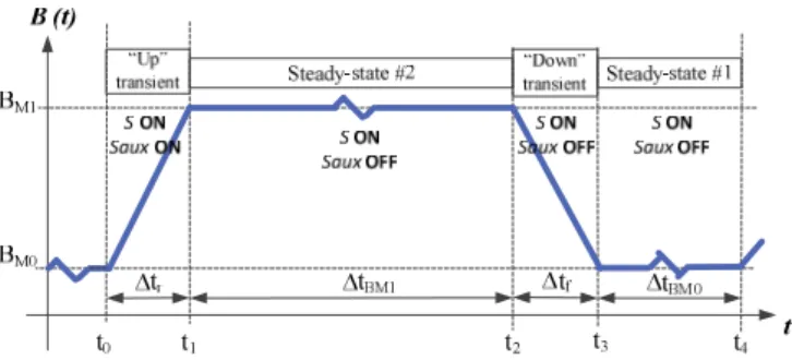
The flux density of a Fast Field Cycling (FFC) Nuclear Magnetic Resonance (NMR) is directly related with the current demanded by the used magnet [1-4]. As typical requirements, the flux density should cycle as shown in Fig. 1 with a ratio of about 0.1 T/ms [5-9]. In addition, from cycle to cycle, the low level of the flux density can be adjusted and the flux density levels should be defined with accuracy.
Fig. 1. Flux density cycle of a FFC NMR relaxometer.
In this paper, the dynamic behavior and flux density control of the FFC NMR power supply in Fig. 2 is analyzed when
testing controllers with two different configurations (PI and PD2I).
Fig. 2. Electric circuit of the power supply. II. CONTROL
The operating modes of the proposed topology are the following [10]:
Up: fast flux density transition from a low level (BM0) to a
high level (BM1);
Steady-state #1: steady-state flux density when the flux density is at the high level, corresponding to the “polarization” level or the “detection level” of a FFC NMR experiment;
Down: fast flux density transition from a high level (BM1) to
a low level (BM0);
Steady-state #2: steady-state flux density when the flux density is at a low level, corresponding to the “evolution” level of a FFC NMR experiment; this flux density level is adjusted from cycle to cycle, according to the experimental requirements.
2014
International Symposium on Power Electronics, Electrical Drives, Automation and Motion
In Fig. 3, the circuit with a closed loop control system is shown.
Fig. 3. Diagram of the circuit with the control system.
In order to understand the running of the proposed solution it is important to refer that: the auxiliary power source Uaux is
only connected during the “Up” transient in order to accelerate the flux density transition [10]; and, commanding the semiconductor S, the magnet current iM can be set adjusting the
collector-emitter voltage VCE.
The gain KB of the Hall Effect circuit depends mainly on
the characteristics of the magnet (B=f(iM)). Considering the
available magnet [10], KB=0.04V/T.
Under these conditions, it is assumed a linear relationship between VCE and the gate-emitter voltage VGE.
∆
∆ (1)
The parameter β=700 is considered based on the characteristics of the semiconductor used and the minimum value of VCE that assures safe operation of the IGBT [10].
According to the Fig. 3 circuit, VGE depends on the
command voltage UC and on the emitter resistance RE.
∆ ∆ ∆ (2)
So that and according to the typical specifications of the FFC NMR apparatus, the flux density should be dynamically controlled considering either a step or a ramp as reference inputs. Under these conditions, two controllers will be tested. A. PD2I controller
The block diagram for a PD2I controller (proportional, derivative and two integral actions) is represented in Fig. 4.
s KI 1 KP S KD s
K
I 2Fig. 4. Block diagram of the PD2I controller.
Being the transfer function of the PI2D controller:
∆
∆ (3)
The global block diagram of the proposed circuit can be simplified as shown in Fig. 5.
s ' A L τ + 1
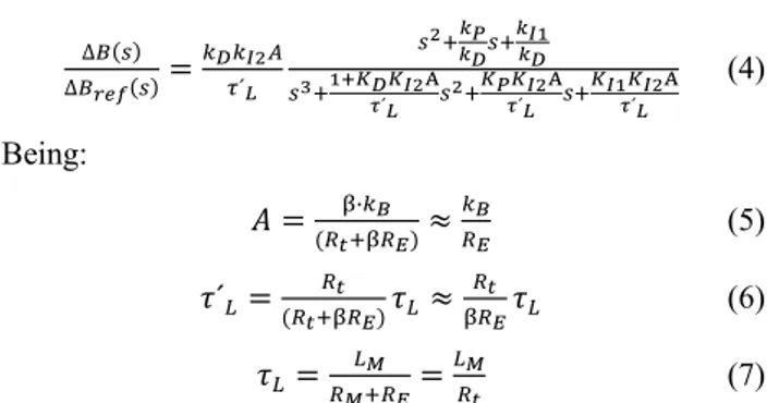
Fig. 5. Block diagram of the proposed circuit with the controller. The global transfer function is:
∆ ∆ ´ A ´ A ´ A ´ (4) Being: · (5) ´ (6) (7) Where LM represents the self-inductance of the magnet RM
is the resistance of the magnet and RE is the emitter resistance.
As first approach, considering KD=0, the transfer function
(4) becomes: ∆ ∆ ´ A ´ ´ ´ A ´ (8) For this type of system, the static speed error should be
minimized. Using the criteria ITAE, the 3rd order optimized
transfer function is given by [11-13]:
,
, , (9)
Based on this approach, the parameters of the control system should be set according the following conditions:
, ´ (10)
,
, ´ (11)
B. PI controller
The typical transfer function of a PI controller (proportional and integral actions) is:
∆
∆ (12)
Using the PI controller, the global closed loop transfer function for the proposed system becomes:
∆ ∆ 1 1 ´ 1 1 1 ´ (13) Assuming that,
´
and 8 (14)
expression (13) can be simplified, being:
∆ ∆ ´ 2 1 ´ ´ (15) In this case, the optimized transfer function can be
represented as:
√ (16)
Considering (15) and (16), the following equations, under optimized conditions, are obtained:
0 2 ´ (17) 0 1 √2 ´ (18)
And joining (17) and (18),
1
√2 ´ 2
´ (19)
The polynomial characteristic of the proposed system is therefore:
0 ´ K (20)
In order to get a stable system, the following condition should be observed:
´ 2
2 1 0 (21)
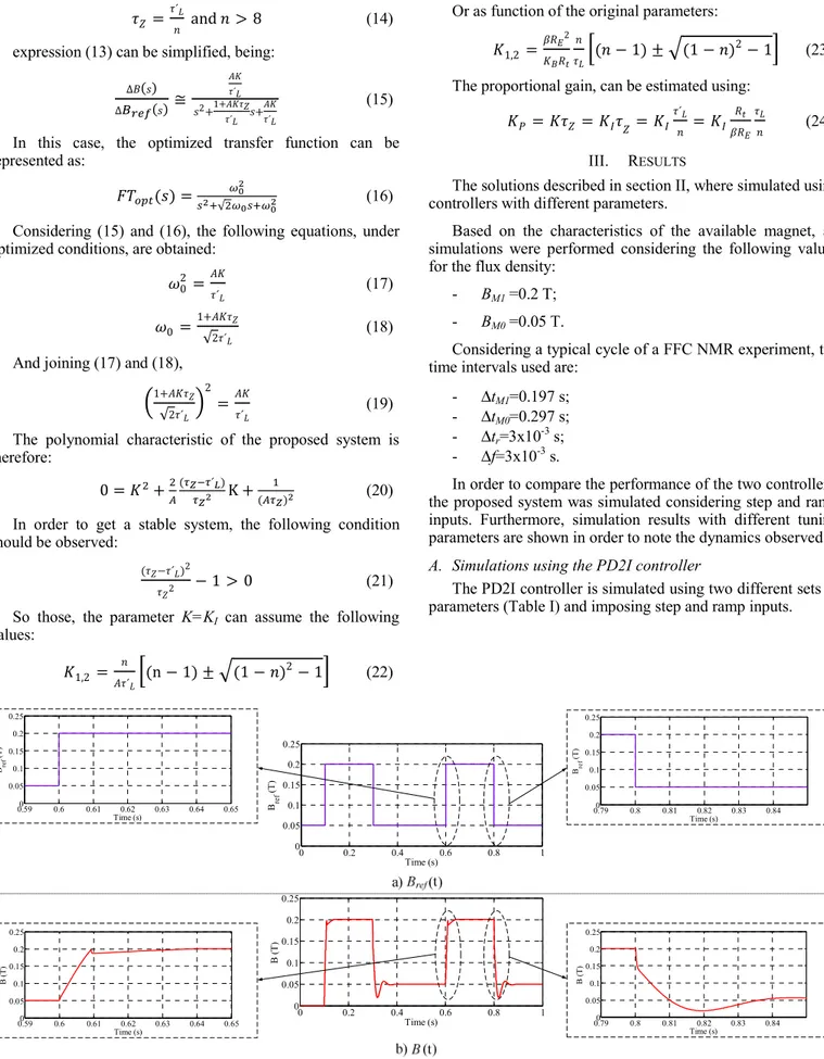
So those, the parameter K=KI can assume the following
values:
1,2 ´ n 1 1 2 1 (22)
Or as function of the original parameters:
1,2
2
1 1 2 1 (23)
The proportional gain, can be estimated using:
´
(24) III. RESULTS
The solutions described in section II, where simulated using controllers with different parameters.
Based on the characteristics of the available magnet, all simulations were performed considering the following values for the flux density:
- BM1 =0.2 T;
- BM0 =0.05 T.
Considering a typical cycle of a FFC NMR experiment, the time intervals used are:
- ΔtM1=0.197 s;
- ΔtM0=0.297 s;
- Δtr=3x10⁻³ s;
- Δf=3x10⁻³ s.
In order to compare the performance of the two controllers, the proposed system was simulated considering step and ramp inputs. Furthermore, simulation results with different tuning parameters are shown in order to note the dynamics observed. A. Simulations using the PD2I controller
The PD2I controller is simulated using two different sets of parameters (Table I) and imposing step and ramp inputs.
0 0.2 0.4 0.6 0.8 1 0 0.05 0.1 0.15 0.2 0.25 Time (s) Bre f (T ) 0 0.2 0.4 0.6 0.8 1 0 0.05 0.1 0.15 0.2 0.25 Time (s) B ( T ) 0.590 0.6 0.61 0.62 0.63 0.64 0.65 0.05 0.1 0.15 0.2 0.25 Time (s) B ( T ) 0.790 0.8 0.81 0.82 0.83 0.84 0.05 0.1 0.15 0.2 0.25 Time (s) B ( T ) 0.790 0.8 0.81 0.82 0.83 0.84 0.05 0.1 0.15 0.2 0.25 Time (s) Bre f (T ) 0.590 0.6 0.61 0.62 0.63 0.64 0.65 0.05 0.1 0.15 0.2 0.25 Time (s) Bre f (T)
0.59 0.6 0.61 0.62 0.63 0.64 0.65 0.05 0.1 0.15 0.2 Time (s) B ( T ) 0.79 0.8 0.81 0.82 0.83 0.84 0.05 0.1 0.15 0.2 Time (s) B ( T ) 0 0.2 0.4 0.6 0.8 1 0 0.05 0.1 0.15 0.2 Time (s) B (T) 0 0.2 0.4 0.6 0.8 1 0 0.05 0.1 0.15 0.2 0.25 Time (s) Bre f (T ) 0.790 0.8 0.81 0.82 0.83 0.84 0.05 0.1 0.15 0.2 0.25 Time (s) Bre f (T) 0.590 0.6 0.61 0.62 0.63 0.64 0.65 0.05 0.1 0.15 0.2 0.25 Time (s) Bre f (T)
Fig. 7. Simulations using a PD2I controller for a step input and the set #2 of parameters. TABLE I. PD2I CONTROLLER PARAMETERS
Set #1 Set #2
KP 6.37 80
KD 0.05 0.05
KI1 1000 1000
KI2 100 5000
The simulations results obtained for the PD2I controller imposing a step input, considering the two parameters sets, are shown in Fig. 6 and Fig. 7.
a) Bref
b) B(t)
Fig. 8. Simulations using a PD2I controller for a ramp input (set #1 of parameters).
In Fig. 8 and Fig. 9 are presented the simulations results for the PD2I controller for a ramp input.
a) Bref
b) B(t)
Fig. 9. Simulations using a PD2I controller for a ramp input (set #2 of parameters).
B. Simulations using the PI controller
In the figures below, simulations performed imposing a step input and a ramp input, respectively, are performed using the following two sets of parameters for a PI controller:
- KP=500; - KI=50000. 0 0.2 0.4 0.6 0.8 1 0 0.05 0.1 0.15 0.2 0.25 Time (s) Bre f (T ) 0 0.2 0.4 0.6 0.8 1 0 0.05 0.1 0.15 0.2 0.25 Time (s) B ( T ) 0 0.2 0.4 0.6 0.8 1 0 0.05 0.1 0.15 0.2 0.25 Time (s) Bre f (T ) 0 0.2 0.4 0.6 0.8 1 0 0.05 0.1 0.15 0.2 0.25 Time (s) B ( T )
a) Bref b) B(t)
Fig. 10. Simulations using a PI controller for a step input.
0.590 0.6 0.61 0.62 0.63 0.64 0.65 0.05 0.1 0.15 0.2 0.25 Time (s) B ( T ) 0.590 0.6 0.61 0.62 0.63 0.64 0.65 0.05 0.1 0.15 0.2 0.25 Time (s) Bre f (T) 0.790 0.8 0.81 0.82 0.83 0.84 0.05 0.1 0.15 0.2 0.25 Time (s) Bre f (T ) 0.790 0.8 0.81 0.82 0.83 0.84 0.05 0.1 0.15 0.2 0.25 Time (s) B ( T ) 0 0.2 0.4 0.6 0.8 1 0 0.05 0.1 0.15 0.2 0.25 Time (s) B ( T ) 0 0.2 0.4 0.6 0.8 1 0 0.05 0.1 0.15 0.2 0.25 Time (s) Bre f (T)
Fig. 11. Simulations using a PI controller for a ramp input.
As it can be observed in the previous figures, both controllers fulfill the requirements of the application. Anyway, considering that fast transients are required, the dynamics observed when imposing step inputs are adequate. Furthermore, the easier tuning and less complexity of the PI controller are factors that should be balanced. So that, in the developed prototype [10, 14], a PI controller was implemented successfully.
C. Experimental results using the PI controller
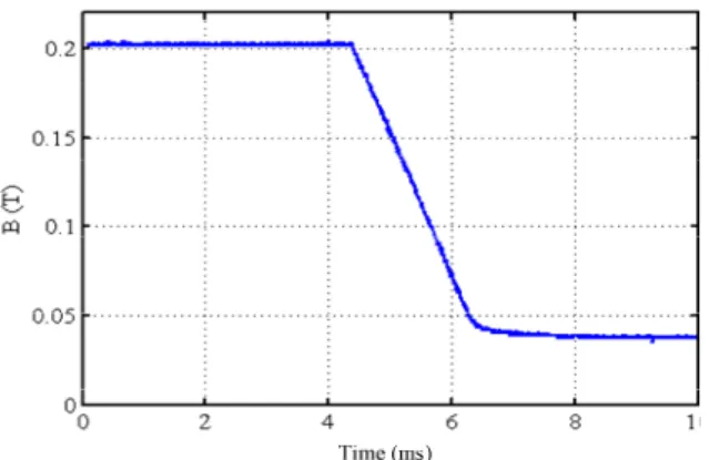
In Fig. 12 and Fig. 13, experimental results for the flux density using a PI controller are shown.
Fig. 12. Experimental “Up” transient using a PI controller for a step input.
0 0.2 0.4 0.6 0.8 1 0 0.05 0.1 0.15 0.2 0.25 Time (s) Bre f (T ) 0 0.2 0.4 0.6 0.8 1 0 0.05 0.1 0.15 0.2 0.25 Time (s) B ( T )
Fig. 13. Experimental “Down” transient using a PI controller for a step input. As it can be observed, the experimental results fulfil the requirements of the application, i.e., fast transients without oscillations.
IV. CONCLUSION
In this paper, simulations results of a FFC NMR power supply controlled using two controllers with different configurations are shown. Both controllers fulfil the requirements of the application, but the option was taken choosing the controller with less complexity and easier to tune since it can be implemented analogically or digitally.
ACKNOWLEDGMENT
This work was supported by national funds through FCT – Fundação para a Ciência e a Tecnologia, under project PEst-OE/EEI/LA0021/2013.
REFERENCES
[1] F. Noack, “NMR Field-Cycling Spectroscopy: Principles and Applications”, Prog. NMR Spectrosc., vol. 18, pp. 171-276, 1986. [2] R. Seitter, R. O. Kimmich, “Magnetic Resonance: Relaxometers”,
Encyclopedia of Spectroscopy and Spectrometry, Academic Press,
London, pp. 2000-2008, 1999.
[3] E. Anoardo, G. Galli, G. Ferrante, “Fast-Field-Cycling NMR: Applications and Instrumentation”, Applied Magnetic Resonance, vol. 20, pp. 365-404, 2001.
[4] R. Kimmich and E. Anoardo, “Field-Cycling NMR relaxometry”,
Progress in NMR Spectroscopy, 44, pp. 257-320, 2004.
[5] J. Constantin, J. Zajicek, F. Brown, “Fast Field-Cycling Nuclear Magnetic Resonance Spectrometer”, Rev. Sci. Instrum., vol. 67, pp. 2113-2122, 1996.
[6] D. M. Sousa, P. A. L. Fernandes, G. D. Marques, A. C. Ribeiro, P. J. Sebastião, “Novel Pulsed Switched Power Supply for a Fast Field Cycling NMR Spectrometer”, Solid State Nuclear Magnetic Resonance, vol. 25, pp. 160-166, 2004.
[7] D. M. Sousa, G. D. Marques, J. M. Cascais, P. J. Sebastião, “Desktop Fast-Field Cycling Nuclear Magnetic Resonance Relaxometer”, Solid
State Nuclear Magnetic Resonance, vol. 38, pp. 36-43, 2010.
[8] A. Roque, S. F. Pinto, J. Santana, Duarte M. Sousa, E. Margato, J. Maia, “Dynamic Behavior of Two Power Supplies for FFC NMR Relaxometers”, IEEE International Conference on Industrial Technology – ICIT 2012, Athens - Greece, 2012.
[9] D. M. Sousa, E. Rommel, J. Santana, J. Fernando Silva, P. J. Sebastião, A. C. Ribeiro, “Power Supply for a Fast Field Cycling NMR Spectrometer Using IGBTs Operating in the Active Zone”, 7th European Conference on POWER ELECTRONICS AND APPLICATIONS, , Trondheim, Norway, pp. 2.285-2.290, 1997.
[10] A. Roque, D. M. Sousa, E. Margato, J. Maia and Gil Marques, “Control and Dynamic Behaviour of a FFC NMR Power Supply - Power Consumption and Power Losses”, IECON 2013 – 39th Annual Conference of the IEEE Industrial Electronics Society, Vienna, Austria, 2013.
[11] K. Ogata, “Modern Control Engineering”, 5th Edition, Prentice-Hall, 2010.
[12] A. G. Redfield, W. Fite, H. E. Bleich, “Precision High Speed Current Regulators for Occasionally Switched Inductive Loads”, Review of
Scientific Instruments, vol. 39, pp. 710-715, 1968.
[13] J. J. D'Azzo and C. H. Houpis, “Linear Control System Analysis and Design: Conventional and Modern”, 4th Edition, McGraw-Hill, 1995. [14] D. M. Sousa, G. Marques and P. J. Sebastião, “Reducing the size of Fast
Field Cycling NMR Spectrometers based on the use of IGBTs”, “IEEE ICIT 2009 - International Conference on Industrial Technology”, Churchill - Australia, February 2009.