Time-resolved optical tomography of functional activation in the adult brain using a supercontinuum laser source

FACULDADE DE CIÊNCIAS

DEPARTAMENTO DE FÍSICA

Time-resolved optical tomography of

functional activation in the adult brain

using a supercontinuum laser source

Tania Roque

Dissertação

Mestrado Integrado em Engenharia Biomédica e Biofísica

Perfil de Sinais e Imagens Médicas

FACULDADE DE CIÊNCIAS

DEPARTAMENTO DE FÍSICA

Time-resolved optical tomography of

functional activation in the adult brain

using a supercontinuum laser source

Tania Roque

Dissertação

Mestrado Integrado em Engenharia Biomédica e Biofísica

Perfil de Sinais e Imagens Médicas

Orientadores Professor Doutor João Pinto Coelho

Professor Doutor Jeremy Hebden

Esta dissertação descreve o projeto de investigação realizado no Department of Medical Physics and Bioengineering da University College of London, cujo tema é a tomografia ótica da ativação funcional no cérebro adulto utilizando um laser supercontínuo.

A imagiologia ótica é uma técnica que consiste em irradiar um volume de interesse com uma fonte luminosa, analisar as propriedades da luz que atravessou esse mesmo vol-ume e reconstruir imagens com base nessa informação. Esta técnica já provou ser útil em diversos campos da ciência e da engenharia, e o seu potencial na área da saúde tem vindo a ser cada vez mais estudado. Atualmente, e no âmbito da Engenharia Biomédica, as suas principais aplicações são a imagiologia funcional do cérebro adulto e do cérebro do recém-nascido, a mamografia ótica, o estudo de tecido muscular e ósseo, e a imagiologia molecular.

Independentemente do tecido em estudo, é a interação da luz com a matéria que per-mite a aquisição de informação biológica, nomeadamente a dispersão e a absorção. A luz é uma forma de radiação eletromagnética e pode ser caracterizada de diversas formas. Uma característica do seu movimento ondulatório é o comprimento de onda, que consiste na distância linear em nanómetros (nm) entre duas cristas da onda luminosa e é uma me-dida do conteúdo energético da luz. Ao deslocar-se num meio, uma fração ou a totalidade da luz pode ser absorvida pela matéria envolvente. Quando este fenómeno – a absorção – ocorre, há uma transferência de energia da onda luminosa para a matéria envolvente. Con-tudo, nem toda a matéria absorve a luz na mesma medida, e é exatamente por isso que a imagiologia ótica é possível. De facto, se dois tecidos diferentes interagirem com a luz de igual forma, não é possível distingui-los numa imagem resultante de imagiologia ótica. Assim, diferentes moléculas apresentam diferentes espectros de absorção de luz. Se uma onda luminosa com um comprimento de onda específico atravessar dois volumes, cada um contendo uma substância com espectro de absorção diferente, a quantidade de energia transferida para cada um desses volumes será diferente. Se, por exemplo, repetirmos a mesma experiência com outro comprimento de onda maior ou com uma maior concen-tração das substâncias no volume estudado, a absorção luminosa já não será a mesma. A imagiologia ótica baseia-se nesta e noutras alterações da onda luminosa, tal como a fase e a amplitude da onda, para criar imagens.

Para tal, é necessário que o sistema de imagiologia possua uma fonte luminosa e detetores de luz. Dependendo das configurações destes dois componentes, é possível categorizar os diversos sistemas de imagiologia ótica. No caso particular do aparelho uti-lizado para este projecto, trata-se de um sistema designado pelo acrónimo MONSTIR, do inglês Multi-channel Opto-electronic Near-infrared System for Time-resolved Image

numa mesma experiência. A luz gerada pelo laser percorre as várias fibras até penetrar nos tecidos. Aí a luz interage com a matéria, sendo que a luz que não foi absorvida acaba por sair e por ser captada pelas fibras óticas. Esse sinal luminoso, que contém a infor-mação biológica que procuramos obter, é encaminhado para um conjunto de atenuadores, detetores e contadores de fotões. Depois ser assim convertido para um formato digital, este sinal é analisado por softwares especializados que extraem a informação necessária para reconstruir imagens. A reconstrução de imagens utilizou um método linear e uma malha tridimensional do volume estudado – o cérebro.

Este aparelho foi desenvolvido no Biomedical Optical Research Laboratory da UCL com o propósito de ser utilizado em ambiente clínico para monitorizar a ocorrência de convulsões em bebés nascidos prematuramente e avaliar a sua resposta aos tratamentos. As convulsões estão relacionadas com um estado de hipoxia cerebral, isto é, com con-centrações de oxigénio no cérebro muito baixas. Podem-se distinguir duas moléculas relevantes neste contexto: a oxihemoglobina, que transporta o oxigénio, e a deoxihe-moglobina, que já forneceu o oxigénio aos neurónios. As concentrações destas duas moléculas são alteradas quando um bebé está em hipoxia cerebral, e esta é a alteração fisiológica que o MONSTIR consegue medir. Esta medição é possível porque a oxihe-moglobina e a deoxiheoxihe-moglobina têm espectros de absorção diferentes. Por exemplo, se iluminarmos o crânio de um bebé com um comprimento de onda que sabemos ser al-tamente absorvido pela oxihemoglobina e se os detetores do MONSTIR detetarem uma elevada fração dessa luz, é sinal que a luz atravessou os tecidos sem encontrar uma con-centração elevada de oxihemoglobina - podemos estar a diagnosticar um caso de hipoxia cerebral.

No entanto, para poder realizar o seu propósito, o MONSTIR precisa de completar uma fase de caracterização e afinação de modo a garantir que a sua utilização em ambi-ente clínico é totalmambi-ente segura e que os dados recolhidos são fiáveis. Uma das questões que se levanta quanto aos seus parâmetros de funcionamento ótimos é sobre os compri-mentos de onda a selecionar. Tal como foi referido acima, o MONSTIR dá-nos a liber-dade de escolher até 4 comprimentos de onda. Quais são os 4 comprimentos de onda que garantem as melhores imagens do cérebro? Esta questão é extremamente importante para a qualidade dos resultados, mas não é óbvia. Uma revisão da literatura sobre a in-vestigação com imagiologia ótica revela que a escolha dos comprimentos de onda muitas vezes não é justificada com um argumento científico. A otimização dos comprimentos de onda utilizados é portanto um tópico que pode ter um impacto significativo nas futuras investigações neste campo. Como tal, decidiu-se testar qual a melhor combinação de 4 comprimentos de onda para a aquisição de imagens do cérebro.

Foi realizada uma experiência num sujeito adulto, saudável, que realizou uma tarefa motora simples. Para manter as fibras óticas junto ao couro cabeludo do sujeito, foi-lhe colocada uma touca normalmente utilizada para encefalografias. Nove fibras óticas foram dispostas sobre o córtex motor esquerdo do sujeito. Para fixar as fibras óticas à touca foi necessário fabricar nove conectores à medida. Desenharam-se os conectores em CAD e recorreu-se a uma impressora 3D para os fabricar. O estímulo motor realizado pelo sujeito consistiu em tocar sequencialmente e repetidamente com cada dedo da mão

criasse habituação à tarefa motora e para permitir a aquisição de um sinal de referência (sem qualquer estímulo). O objetivo desta experiência era comparar a qualidade do sinal resultante da ativação do córtex motor dependendo da nossa escolha de 4 comprimentos de onda. Foram testados 12 comprimentos de onda diferentes que, ao serem combinados em conjuntos de 4, resultaram em 495 diferentes combinações de 4 comprimentos de onda. Estas combinações foram analisadas com 3 métodos diferentes.

O método A tem recurso a um algoritmo baseado na lei de Beer-Lambert modificada e adaptada à imagiologia ótica. O output deste algoritmo é a variação na concentração dos dois cromóforos estudados, oxihemoglobina e deoxihemoglobina. As 495 combinações de 4 comprimentos de onda são testadas neste algoritmo, e aquilo que procuramos são aquelas que produzam um maior sinal, ou seja, uma maior variação na concentração de oxihemoglobina e deoxihemoglobina. Espera-se que a obtenção de um maior sinal irá levar a melhores imagens.

O método B também utiliza o algoritmo baseado na lei de Beer-Lambert modificada, mas desta vez o seu output é comparado com um modelo teórico que prevê os valores de concentração de oxihemoglobina e deoxihemoglobina. Antes de tudo, este modelo teórico é criado para se adaptar o melhor possível aos nossos dados experimentais, e depois é comparado aos 495 possíveis outputs do algoritmo. A melhor combinação é a responsável pela geração do output mais próximo do modelo teórico.

O método C consiste primeiro na reconstrução de 495 imagens, cada uma delas resul-tante de uma combinação diferente de 4 comprimentos de onda. É também reconstruída uma imagem ideal que contém informação dos 12 comprimentos de onda. Esta é consid-erada a melhor imagem possível e procuramos a imagem de 4 comprimentos de onda que lhe seja mais semelhante. Esta medida de semelhança é feita com recurso à raíz do erro quadrático médio.

Para cada um destes métodos é feita uma classificação de #1 a #495 das combinações de comprimentos de onda. As melhores e as piores 5 combinações de cada método foram então analisadas em maior profundidade. Conclui-se que o método mais adequado para a classificação das combinações de comprimentos de onda é o método C, visto que em última análise aquilo que pretendemos são as melhores imagens possíveis. A melhor combinação de comprimentos de onda com este método foi 690, 790, 810 e 840 nm. Verificou-se também que os comprimentos de onda utilizados na literatura são na sua grande maioria comprimentos que se encontravam bastante baixos na classificação que fizemos. No futuro, é importante aperfeiçoar o método C, repetir esta experiência com outros sujeitos e estudar outros cromóforos.

A dissertação está dividida em 4 capítulos. O primeiro consiste numa introdução que explora as propriedades óticas dos tecidos biológicos, a engenharia por detrás da imagi-ologia ótica e o state-of-the-art das escolhas dos comprimentos de onda na imagiimagi-ologia ótica. O segundo capítulo descreve os procedimentos para a aquisição de dados, portanto a vertente mais prática deste projecto. O terceiro capítulo apresenta os dados obtidos ao mesmo tempo que explora a metodologia da análise de dados. No quarto capítulo é feita a discussão dos dados, são apresentadas as limitações deste projeto, e as conclusões.

Diffuse optical imaging (DOI) is finding widespread application in the study of human brain activation. However, the process of wavelength selection is unclear and may lead to choices that negatively affect the accuracy and reliability of the data.

This thesis describes a method to empirically determine the combination of four near-infrared (NIR) wavelengths that yields the best images of functional activity in the brain. An experiment was designed to quantify changes of chromophores oxyhaemoglobin and deoxyhaemoglobin in the motor cortex of a healthy adult subject using UCL’s second generation optical imaging device, MONSTIR. This devices allows us to use four wave-lengths simultaneously. A set of twelve was tested and recombined into 495 combina-tions of four wavelengths. This data was analysed with three methods that ranked the four-wavelength combinations according to different conditions. Method A looked for the largest change resulting from a modified Beer-Lambert law algorithm. Method B favoured the combinations whose output of the same algorithm was closest to a theoreti-cal model. Method C compared the 495 four-wavelength images to a twelve-wavelength image (a gold-standard) and ranked the wavelength combinations by looking for the min-imum root-mean-square error between each pair of images.

We concluded that the most adequate method is method C because it provides with the best images. The best set of wavelengths obtained was 690, 790, 810 and 840 nm. These results are specific to the imaging device used, however our general method can be applied to other optical imaging systems.

Keywords: Optical imaging, Functional imaging, Near-infrared, Optimization, Wave-length, Motor cortex, Oxyhaemoglobin, Deoxyhaemoglobin, MONSTIR, Supercontin-uum laser

I wish to thank all the people who crossed my path throughout this year-long project. I am extremely grateful to my UCL supervisor Professor Jem Hebden who gave me the opportunity to work on this project and who always provided me with his precious time and guidance. Also, this thesis would have been impossible without the continuous help and dedication of Dr. Robert Cooper, to whom I am immensely thankful. You’ve secured a regular income of Portuguese pastries.

I would like to thank my FCUL supervisor Professor João Pinto Coelho for his good ad-vice and his care when I forget to reply to his emails.

I’m very grateful to Dr. Nick Everdell, Dr. Harsimrat Singh, Dimitrios Airantzis and Elliott Magee for answering to my silly enquiries in the lab. Thanks to you and to Dr. Robert Cooper, I’ve learnt how to work with a time-resolved optical imaging device, a glue gun, heat shrink and blue tack.

I want to thank everyone from UCL’s Department of Medical Physics and Bioengineering who welcomed me. Thank you for making me feel truly at home and for not judging my late arrivals at the lab everyday.

I wish to thank everyone that truly turned my stay in London into one of the best expe-riences of my life. I can’t express how important it all was for me. Clément Godard and Sara Reis, your support was so much more than what I could expect.

I would like to express my gratitude to my friends who always stood by my side despite the distance: Marta Silva, André Guerra, Rita Marques, Marisa Marques and my dear brother Valentin Roque. None of this would have been possible without the incredible support and patience of my parents, Rui and Catherine Roque.

I also thank my old computer for holding up to this ultimate challenge, and my beloved cat Biacha for laying on my lap and therefore keeping me from moving away from the computer during the writing process.

Resumo IV

Abstract V

Acknowledgements VI

List of Acronyms IX

List of Figures XII

List of Tables XIII

1 Introduction 1

1.1 Motivation . . . 1

1.2 Fundamentals of biomedical optics . . . 1

1.2.1 Light properties . . . 1

1.2.2 Light-tissue interaction . . . 2

1.2.3 Modified Beer-Lambert law . . . 6

1.3 The brain . . . 6

1.3.1 Brain tissue properties . . . 6

1.3.2 Electrical and vascular activity . . . 7

1.3.3 Motor cortex . . . 8

1.4 Near infrared imaging . . . 10

1.4.1 Near infrared imaging signal . . . 10

1.4.2 Types of near infrared instrumentation . . . 11

1.4.3 MONSTIR . . . 16

1.4.4 10-20 system . . . 19

1.5 Image reconstruction . . . 19

1.6 Wavelength choice . . . 21

2 The experiment 22 2.1 Goal of the experiment . . . 22

2.2 Array design and construction . . . 22

2.3 Experiment design . . . 23

2.4 Additional information on the procedure . . . 27

2.4.1 Characterisation done before the experiment . . . 27

3 Data analysis 30

3.1 Data processing . . . 30

3.2 Results . . . 33

3.2.1 Data validation . . . 33

3.2.2 A - Largest chromophore change . . . 37

3.2.3 B - Comparison with theoretical model . . . 42

3.2.4 C - Comparison with gold-standard image . . . 45

3.2.5 Comparison between methods . . . 50

4 Discussion 55 4.1 Discussion of results obtained with methods A, B and C . . . 55

4.2 Discussion of results obtained with method C . . . 57

4.3 Limitations and future work . . . 58

4.4 Conclusion . . . 58

MONSTIR Multi-channel Opto-electronic Near-infrared System for Time-resolved Im-age Reconstruction

NIR near-infrared

BORL Biomedical Optical Research Laboratory NIRS (near-infrared spectroscopy

BOLD blood oxygen level dependence DOI diffuse optical imaging

PET positron emission tomography

SPECT single positron emission computed tomography MEG magnetoencephalography

fMRI functional magnetic resonance imaging ERP event related potentials

EEG electroencephalography

AOTF acousto-optical tunable filters

TCSPC time correlated single photon counting VOA variable optical attenuator

PMT photomultiplier tubes

TPSF temporal point spread function CW continuous wave

FR frequency-resolved APD avalanche photodiodes DPF differential path length factor

FEM finite-element method ATP adenosine-tri-phosphate CBF cerebral blood flow

CMRO2 cerebral metabolic rate of oxygen HbO₂ oxyhaemoglobin

HbR deoxyhaemoglobin HbT total haemoglobin ANOVA analysis of variance SNR signal-to-noise ratio RMSE root-mean-square error

1.1 Light reflection and refraction . . . 2

1.2 Absorption spectra of oxyhaemoglobin and deoxyhaemoglobin . . . 4

1.3 Absorption spectrum of water . . . 4

1.4 Diagram of light scattering through a layer of cells . . . 5

1.5 The aerobic metabolism of glucose to ATP following the Kreb’s cycle . . 7

1.6 Location of the human motor cortex in the brain . . . 9

1.7 Map of the body in the human brain . . . 9

1.8 Typical NIR signal resultant from functional brain activation . . . 11

1.9 NIR spectroscopy, topography and tomography . . . 12

1.10 Representation of a frequency domain NIRS measurement . . . 13

1.11 The influence of the tissue optical characteristics on TPSF shape . . . 14

1.12 Comparison of spatial sensitivity and temporal sensitivity of six neu-roimaging methods . . . 15

1.13 MONSTIR . . . 16

1.14 Schematic functioning of MONSTIR . . . 17

1.15 Diagram of the output optics of MONSTIR . . . 18

1.16 Comparison of the output power of supercontinuum lasers and other light sources . . . 18

1.17 The international 10-20 system . . . 20

2.1 Array design . . . 23

2.2 Cap on subject . . . 24

2.3 Customised sockets with prism . . . 24

2.4 Temporal scheme of one acquisition of the experiment . . . 25

2.5 Scheme of full data acquisition . . . 26

2.6 Wavelengths used for data acquisition . . . 26

2.7 Power output of the MONSTIR fibres and the supercontinuum laser . . . 28

3.1 Diagram of the methods used to analyse the data . . . 32

3.2 Comparison of active and rest areas under all the 3840 TPSFs . . . 34

3.3 Comparison of active and rest areas under 10 active and 10 rest TPSFs . . 36

3.4 Meantime and intensity against fibre separation . . . 37

3.5 Change in intensity measured with different channels . . . 39

3.6 Average of 10 TPSFs measured with different channels . . . 40

3.7 Ranking of combinations of wavelengths for method A . . . 42

3.8 Theoretical model output . . . 43

3.12 Ranking of combinations of wavelengths for method C . . . 47 3.13 Images reconstructed for oxyhaemoglobin using the best and worst

wave-length combinations for method C . . . 48 3.14 Images reconstructed for deoxyhaemoglobin using the best and worst

wavelength combinations for method C . . . 49 3.15 Comparison of the best and worst wavelength combinations for methods

A, B and C . . . 51 3.16 Images reconstructed for oxyhaemoglobin using the best and worst

wave-length combinations for method A . . . 52 3.17 Images reconstructed for oxyhaemoglobin using the best and worst

wave-length combinations for method B . . . 53 3.18 Comparison of the average and range of wavelength combinations from

2.1 Three sets of four wavelengths used for data acquisition . . . 27 3.1 Result of the ANOVA test applied to the data acquired with all

wave-lengths and channels . . . 33 3.2 Result of the ANOVA test applied to data acquired with one wavelength

and one channel . . . 35 3.3 Relationship between intensity change measurement and fibre distance . . 38

Introduction

1.1

Motivation

A Multi-channel Opto-electronic Near-infrared System for Time-resolved Image Recon-struction (MONSTIR) was developed at the UCL’s Biomedical Optical Research Lab-oratory (BORL). This time-resolved optical imaging device was designed to diagnose seizures in premature babies and monitorize their response to treatment. It gives us the possibility of recording data at any four wavelengths simultaneously. When doing optical imaging, the tissue is illuminated and the properties of the collected light are analysed. The choice of the wavelength to use when irradiating the tissue is very important for the quality and reliability of the results. However, this choice is not obvious and a literature review reveals that the choice of wavelengths in optical imaging experiments isn’t always scientifically justified. The purpose of my project was to empirically determine the com-bination of four NIR wavelengths that yields the best images of functional activity in the brain. The studied chromophores were oxyhaemoglobin and deoxyhaemoglobin.

The present thesis describes the work done during my 8-month internship at BORL. This work consisted on the characterization of MONSTIR, the acquisition of images of the healthy adult brain during a simple motor experiment and the analysis of the data.

1.2

Fundamentals of biomedical optics

1.2.1

Light properties

A light wave is a sinusoidal function such as the following:

x(t) = A. sin(2π f t + ϕ) (1.1) The function varies with time, and A, f and ϕ are constant parameters called the am-plitude, frequency, and phase of the sinusoid. The square of the wave amplitude A is proportional to irradiance - named intensity in most branches of physics - which is the power of electromagnetic radiation per unit area incident on a surface (W /m2). Power is a property of the light source that describes the rate at which light energy is emitted by the source, and is often measured in units of watts (W ). When increasing the power or intensity of a light beam, one is increasing its amplitude and therefore the number of

Figure 1.1: Light reflection and refraction. [27]

photons emitted. The frequency f of a light wave is inversely proportional to its wave-length. When varying these magnitudes one is not changing the number of photons, but their energy: higher wavelengths are more energetic than lower wavelengths. The phase is the fraction of the wave cycle which has elapsed relative to the origin.

1.2.2

Light-tissue interaction

The encounter of light with the surface of a bulk matter can result in either reflection or refraction. The propagation of light in a given type of media can result in scattering and absorption. These four events will be described in the context of optical brain imaging. 1.2.2.1 Reflection and refraction

Reflection of light may occur whenever light travels from a medium of a given refractive index into a medium with a different refractive index. The law of reflection states that θ i = θ r, in other words, the angle of incidence equals the angle of reflection (see figure 1.1). If the light is incident on the tissue at 0◦, maximum light will penetrate the tissue. However, when performing optical brain imaging, the surface (hair, skin, scalp) of the bulk volume (head) is rough at a microscopic level and therefore have many different normal lines. As a result, the reflected rays bounce off in many angles rather than in just one angle. This is known as non-specular or diffuse reflection, in opposition to specular reflection that occurs on a mirror, for instance.

When light is transmitted from one medium to another, the difference in the refractive index results in a change in the speed of light. If this transmission happens at any angle other than 0◦or 90◦, the difference in the refractive index also results in a change of the light’s direction. This change is responsible for the bending of light, or refraction, and is explained by Snell’s law: the ratio of the sines of the angles of incidence and refraction is equivalent to the ratio of phase velocities in the two media. This phenomena results in the

phase shift of wavefront points as their velocity changes within media of different optical properties. Just as for reflection, the roughness of biological tissues’ surface generates refracted rays in multiple directions under the tissues’ surface. In practice, when illumi-nating a tissue for optical imaging purposes, the effort is to have an incidence angle of 0 ◦_{so that the fraction of light that enters the tissue is maximized. Then, usually a fraction} of the light is reflected from the interface and the remainder is refracted. [25, 30]

1.2.2.2 Absorption and scattering

Absorption and scattering are the optical events exploited for medical diagnostic in the NIR range. When the energy associated with the incident infrared radiation dissipates in the medium, it does so by transferring heat to the surrounding tissue - this process is known as absorption. The heat production occurs in particular within the infrared re-gion of the electromagnetic spectrum because the frequencies covered by its radiation are comparable to the natural frequencies at which atoms or molecules vibrate. The result is a resonance around the natural frequencies and energy (a photon) is transferred from the incident field to the medium. The overall effect of absorption is therefore a reduction in the intensity of the light beam crossing the system, hence the ratio of absorbed and incident intensities in the Beer-Lambert law (equation (1.2)).

I I₀ = e −µa(λ )x _(1.2) µa(λ ) = n

∑

0) is proportional to the concentration of the compound in the solution

(ci) and the optical path length x, which is the distance travelled in the medium. For a medium such as the brain, the absorption coefficient of the medium µais the combination of many different optically absorbing substances - the chromophores. The most present are water, haemoglobin, lipids, melanin and cytochrome oxidase. The expression of the absorption coefficient for n different substances in the brain tissue is therefore the linear sum of the individual specific absorption coefficient α(λ ) (with units cm−1) multiplied by the respective concentrations c, as equation (1.3) shows.

Focusing on some of the chromophores mentioned above, haemoglobin is typically present as either oxyhaemoglobin (HbO2) or deoxyhaemoglobin (HbR), depending on being bound or not to oxygen. The optical absorption of oxy and deoxyhaemoglobin for NIR radiation is represented in figure 1.2, which shows an optical window between 600 and 1000 nm, where absorption is lower. This optical window is what justifies the use of wavelengths between 600 and 900 nm (approximately) in optical imaging because less absorption by the tissue means that scattering is the most dominant light-tissue interaction in this range. Therefore the propagating light has its maximum depth of penetration in tissue and is able to collect more biological information. At 800 nm is the isobestic point where oxy and deoxyhaemoglobin show the same absorption value. Figure 1.3 shows the absorption spectrum of water - this is a relevant chromophore as it is present in very high concentrations in the human body. The absorption spectrum of water (which is very close

to that of lipids) exhibits a marked increase in absorption of light at wavelengths greater than approximately 900 nm. Once again, this supports the use of the NIR wavelengths for the study of soft tissues, as light will penetrate further than if we used higher wavelengths.

Figure 1.2: Absorption spectra of oxyhaemoglobin and deoxyhaemoglobin. [5]

Figure 1.3: Absorption spectrum of water. [5]

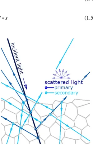
The events that result in a photon’s change of directionality or energy are known as elastic or inelastic scattering, respectively. Scattering is by far the dominant interaction of NIR light with tissues, and elastic scattering is the dominant type of scattering. The

scattering arises due to a relative refractive index mismatch at the boundaries between two media or structures, e.g. between the extracellular fluid and the cell membrane, and can therefore happen successively within the tissue (as figure 1.4 illustrates) until the photons arrive back at the surface or until they are absorbed. The attenuated light intensity due to a single scattering is represented on equation (1.4), where x is the optical path length. The scattering coefficient µs is the probability that a photon will undergo a scattering event per length of medium, and is computed by the product of the scattering cross section of the particles (s) and the number density of particles (N).

I I₀ = e

−µsx _(1.4)

µs= N ∗ s (1.5)

Figure 1.4: Light scattering through a layer of cells; the polygons’ countours are the cells’ membranes. [16]

As soon as the light has entered the tis-sue, the occurrence of multiple scattering events creates an isotropic distribution of light, which contrasts with the initial well-defined path of laser light commonly used in optical imaging. In terms of modelling, it is then necessary to consider the proba-bility of a photon being scattered in a given direction at each interaction. The probabil-ity of a photon incident along a unit vector pbeing scattered into a direction q is de-scribed by the phase function f (p, q). In isotropic media, this probability won’t de-pend on direction p, but on the angle be-tween p and q - referred to as the scat-tering angle e. The phase function can then be re-written as a function of the co-sine of the scattering angle. By calculating the mean cosine of e (that is, g), one can characterize the anisotropy of tissue scat-tering. The equation below represents the reduced scattering factor, which includes g, and measures the effective number of isotropic scatters per unit length.

µ_s0= µs(1 − g) (1.6) The anisotropy of biological tissues is in the range 0.69 > g > 0.99 , whose values demon-strate the predominantly forward direction in which scatter occurs. However, the high values of µslead to an isotropic distribution after the light has travelled a few millimetres. [9, 5, 13]

1.2.3

Modified Beer-Lambert law

In a highly scattering medium the photon path length within tissue increases, and there-fore the probability of absorption substantially increases as well. So in media where both scattering and absorption take place the Beer-Lambert law equation must be modified to take into account two phenomena. First, the photon path length is increased due to the scattering events; second, a part of the photons are rendered undetectable by being scat-tered away from the detector. The modified Beer-Lambert law fulfils these requirements:

I I₀ = e

−µa(λ )Dx+G _(1.7)

However, two assumptions that are clearly inadequate for most biological media have to be made: scattering is constant and the medium is homogeneous. In equation (1.7), D is known as the differential path length factor (DPF) and considers the first stated phe-nomenon. DPF is a scaling factor for the geometrical distance x and is dependent upon the reduced scattering coefficient µ_s0, the absorption coefficient µa(λ ) and the geometry of source and detector. The DPF has been measured in the adult head using both the UCL time of flight system and the UCL intensity modulated optical spectrometer, and a value of approximately 6 was obtained - this value can vary with age, gender and optode position on scalp. This means the euclidean distance between the point where the pho-ton is released and the point where it is detected is increased roughly 6 times due to the scattering events that occur in between. [13] G depends upon the geometry of the set-up and the scattering coefficient of the interrogated tissue, and represents the loss of intensity due to scattered photons that do not reach the detector. This factor is very difficult to cal-culate, making it impossible to solve equation (1.7). However, by making more than one measurement and by considering that G does not vary during the measurement period, one can record changes in the attenuation of NIR light over the medium. The attenuation change between state 1 and state 2 is:

lnI2 I₀− ln I₁ I₀ = ln I₂ I₁ = (∆µa(2−1)(λ ))Dx (1.8) Due to the subtraction, G no longer figures in the equation. Given that we compute Dx, that we use a device which measures lnI2

I1 (the amount of light lost through the medium)

and that ∆µ_a(2−1)= ∑ni=1αi∗ ∆ci, equation (1.8) gives us the change in the concentration of the chromophores. [13, 9] Section 1.4.1 explores how the change of each specific chromophore is computed.

1.3

The brain

1.3.1

Brain tissue properties

Biological tissue is an inhomogeneous and anisotropic medium made up of many different structures and substances. For the brain, these substances are water (77 to 78%), lipids (10 to 12%), protein (8%) and some carbohydrates and salts. Besides the brain itself, the intracranial space contains blood (10%) and cerebrospinal fluid (10%). This cavity is enclosed by the skull and a layer of skin, which are highly scattering tissue. [22]

Figure 1.5: Overview of the aerobic metabolism of glucose to ATP following the Kreb’s cycle. [7]

1.3.2

Electrical and vascular activity

As the center of the nervous system, the brain is mostly made of neurons, among other types of cells. Due to the capacity of polarization of their membranes, neurons are electri-cally excitable cells. This polarization occurs due to the an organized movement of ions in and out of the cell, thus creating a potential between the intracellular and extracellular spaces. The transient polarization of the membrane, when the electrical membrane po-tential of a cell rapidly rises and falls, is a short-lasting event called action popo-tential. It is through action potentials that the information is processed and transmitted from neuron to neuron. This phenomenon is known as the neuron’s electrical response, which can be studied with techniques such as electroencephalography (EEG).

Another type of neural response with more relevance to this work is the vascular response. Brain performs work by consuming adenosine-tri-phosphate (ATP) energy, but it first needs to produce this ATP from blood glucose. This process starts in the cytosol (the liquid inside cells) and continues inside the mitochondria (a cell organelle), and is outlined in figure 1.5.

The first step is called glycolysis and takes place in the cytosol. The blood glucose that enters the cell thanks to the presence of insulin is metabolised to pyruvate. 2 NADH molecules are generated in the process, among other products. In the mitochondria, the pyruvate is converted to Acetyl-CoA, which is an input for the citric acid cycle. The citric acid cycle, or Krebs cycle, is a complex series of chemical reactions used by all aerobic or-ganisms to generate energy (ATP) through the oxidization of acetates into carbon dioxide. Focusing on the oxidization of acetates, it is a process called oxidative phosphorylation. The acetates in question are NADH and FADH2molecules that will be oxidized into their reduced states, NAD- and FAD. Three NADH molecules (resultant from the glycolysis) and one FADH2 molecule work as electron donors and 6 O2 molecules are electron ac-ceptors, thus creating an electron transport chain that only works if oxygen is present. The

terminal electron acceptor of the mitochondrial respiratory chain is cytochrome oxidase. [8]

The electron transport chain powers the pumping of protons out of the mitochondrial matrix, creating an electric potential gradient that provides the driving force for ATP synthesis by the ATP synthase enzyme. This enzyme contains a rotor subunit that sets up the assembling of subunits for ATP synthesis. Most of the ATP molecules are produced this way; in fact, the oxidation of each NADH molecule produces 2.5 ATP molecules, and the oxidation of each FADH2produces 1.5 ATP molecules. One molecule of glucose is equivalent to 30-32 ATP molecules. [36]

Optical neuroimaging works on the basis that the electrical and vascular responses are tightly coupled, influencing each other through a process called neurovascular coupling. Repeated neuronal firing requires ATP to power the active transportation of charged ions across the cellular membrane, which in turn requires glucose and oxygen.

At steady state, the amount of ATP used is equal to that produced. There is a lin-ear relationship between oxygen consumption (in the electron transport chain) and ATP production. The oxygen consumption is therefore a good indicator of the overall energy metabolism. The input of oxygen to the tissue is assured by the blood that flows through the surrounding vessels. This flow, known as cerebral blood flow (CBF), is adjusted to the rate at which oxygen is consumed from the blood, known as the cerebral metabolic rate of oxygen (CMRO2). This expresses a general physiological principle: when function in-creases so does the necessity for oxygen and substract, and flow is accordingly increased. The change in flow is possible because of glutamate, a neurotransmitter released by active excitatory neurons. Glutamate is indeed involved in the dilation of the blood vessels and smooth muscle surrounding the neurons with increased function, allowing greater blood flow. Oxygen is transported around the body in blood by the molecule haemoglobin, a protein. The measurement of changes in concentrations of oxyhaemoglobin and deoxy-haemoglobin can provide us with information about localised tissue oxygenation. A local change in haemoglobin concentrations in the brain implies a change in the local oxygen demand, which in turn is related to the activity of the surrounding neurons. [31, 29]

1.3.3

Motor cortex

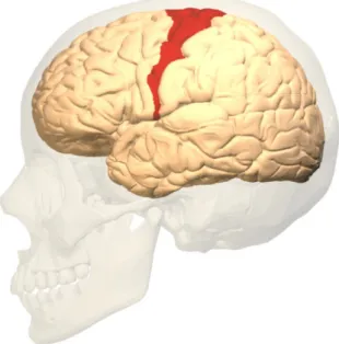
In the light of the experiment described in section 2, it is in the motor cortex that we are looking for changes in neuron activity - it is therefore useful to explain its location. The motor cortex is the region of the cerebral cortex involved in the planning, control, and execution of voluntary movements. Among its several parts, the primary motor cortex is the main contributor to generating neural impulses that pass down to the spinal cord and control the execution of movement. This brain region is located, in humans, in the posterior portion of the frontal lobe (see figure 1.6) and contains large neurons known as Betz cells. Betz cells, along with other cortical neurons, send long axons down the spinal cord, which connects to the muscles. The primary motor cortex contains a rough map of the body (figure 1.7), with different body parts controlled by partially overlapping regions of cortex arranged from the toe (at the top of the cerebral hemisphere) to mouth (at the bottom) along the central sulcus. Each cerebral hemisphere contains a map that controls mainly the contralateral (opposite) side of the body. [28]

Figure 1.7: Map of the body in the human brain. The cerebral cortex has been “inflated” to show the results more clearly. Movements of different body parts evoked activity in the primary motor cortex (left of the central sulcus, shown by the arrow) and primary somatosensory cortex (right of the central sulcus). Although different body parts activated overlapping areas of cortex, only the strongest activations are indicated. [24]

1.4

Near infrared imaging

The previous two sections explained the relationship between chromophores and light, and between chromophores and brain activity. This section explains how to obtain infor-mation about brain activity using optical imaging.

1.4.1

Near infrared imaging signal

The chromophores of interest when doing optical brain imaging are the ones that vary over the period of a measurement or experiment. Water, lipids and melanin are expected to remain constant throughout a short period of time, and are thus responsible for the baseline or background signal. Oxyhaemoglobin, deoxyhaemoglobin and cytochrome ox-idase have a physiological interest when doing functional studies of the brain using optical imaging. Cytochrome oxidase is an enzyme that contains four redox active metal centres; one of these, the binuclear Copper A centre, has a strong absorbance in the near–infrared. However, the fact that the concentration of this centre is less than 10 per cent of that of haemoglobin means that its detection is not a trivial matter, and is commonly neglected in (near-infrared spectroscopy (NIRS) measurements. [8] Due to the fact that the work here presented focuses on the chromophores oxy and deoxyhaemoglobin, cytochrome oxidase won’t be explored in further detail.

For these two chromophores, and considering equations (1.3) and (1.8), the total aborption coefficient change is

∆µa(λ ) = αHbO2(λ ) ∗ ∆cHbO2+ αHHb(λ ) ∗ ∆cHHb (1.9)

However, in order to find the two unknowns, that is, the change in concentration of both chromophores (∆cHbO2 and ∆cHHb), one needs to solve two or more of these equations

simultaneously. It is possible to create more equations by using simultaneously two or more wavelengths in each measurement.

∆µa(λ1) = αHbO2(λ1)∆cHbO2+ αHHb(λ1)∆cHHb (1.10)

∆µa(λ2) = αHbO2(λ2)∆cHbO2+ αHHb(λ2)∆cHHb (1.11)

As explained in section (1.2.3), the reliable reconstruction of the absolute optical prop-erties is very difficult. An accurate knowledge of the interrogated volume and of the po-sitions of the sources and detectors is required, presenting a challenge when obtaining data from the head, for instance. This problem is overcome by reconstructing images us-ing differences in data resultus-ing from a change in optical properties. Difference imagus-ing is achieved by scanning the interrogated tissue before and after a change in the cerebral blood volume and/or oxygenation. [2] Because we are seeking to measure a change in oxy and deoxyhaemoglobin concentration, we need to create an external stimulus that we assume to increase the activity of the neurons in the specific region of the brain being studied. The changes are expected to be seen when comparing this data with the one acquired without a stimulus. Figure 1.8 shows the typical response measured with NIR imaging when the stimulus had the desired effect.

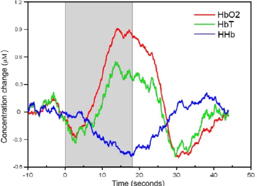
Figure 1.8: Typical NIR signal in result of functional brain activation, showing the con-centration change of oxyhaemoglobin, deoxyhaemoglobin and HbT. The duration of the stimulus is represented by the gray area. (Meek et. al, 1995)

It shows a marked increase in oxyhaemoglobin and a decrease in deoxyhaemoglobin. The sum of both results in an increase in HbT. We know that a change in neuronal activity is related not only to a change in the consumption rate of the oxygen present in blood (CMRO2) but also in the amount of blood reaching the neurons (CBF). The reason for the signal in figure 1.8 is that even though we know there is a change in CMRO2 occurring, the overcompensation in CBF is such that it masks the change in oxygen consumption. In fact, Fox et al. (1986) found that the ratio of the increase in CBF to the increase in CMRO2is approximately 6 for a somatosensory stimulation task.

Analysing the time scale, one can see that just after the start of the stimulus there is a decrease in HbO2and an increase in HHb. This is thought to be due to the response time (around 5 seconds) of the vascular response. Between 5-10 seconds following the end of the stimulus there is a post-stimulus undershoot in HbO2.

1.4.2

Types of near infrared instrumentation

NIR instrumentation can be separated into spectroscopy, topography and tomography according to their sources and detectors configuration, and into continuous wave (CW) systems, frequency-resolved (FR) systems and time domain systems depending on what information is recorded. All of them rely on the changes of NIR light absorbance by the tissues’ chromophores but due to the fact that scattering is the dominant photon-matter interaction, they all belong in the diffuse optical imaging (DOI) category.

Figure 1.9: From left to right: NIR spectroscopy, topography and tomography. Figure courtesy of J C Hebden.

1.4.2.1 Spectroscopy, topography and tomography

Spectroscopy, usually referred to as NIRS, only relates information acquired from one source and one detector. Even when multi-channels are used, a series of one source to one detector spectroscopic measurements are obtained. The light that reaches the detector is diffusively reflected by the tissue. Topography is based on the use of a planar array of sources and detectors that measures the diffusively reflected light present underneath it. The topographic maps obtained carry some information to produce 3D image but with a limited depth. Unlike the two previous modalities, optical tomography requires direct transmission of light so that a full 3D image can be generated. For this to be possible, source and detectors have to be positioned opposite one another, so that the light can cross the whole tissue. On the head and until now, this technique is mostly applied on babies because they allow for a reasonable source-detector distance. The differences between these 3 techniques are illustrated in figure 1.9.

1.4.2.2 Continuous wave systems

In CW systems, light is emitted at a constant intensity and the differences between mea-sured attenuations are recorded. All meamea-sured changes are recognized as changes in ab-sorption because since it is not possible to study the effects of scattering with CW systems, this effect is considered constant.

One disadvantage of a CW system is that, for a suitably brief acquisition time, it only get signals coming from areas directly underneath the detectors. The depth of reach of the CW signal is proportional to the distance between the source and detector: a source-detector pair separated by a distance d will only be sensitive to a depth of approximately d/2, although this value varies with the datatype and is valid for systems other than CW. [1] The majority of continuous wave systems employs avalanche photodiodes (APD)s as the light detector and typically operates with source detector separations of between 15 and 45 mm. This distance is large enough to have a good chance of sampling brain tissue, but small enough to allow a suitable amount of light to be detected. However, larger

source-detector separations can be used if more sensitive and more expensive detecting systems, such as PMTs, are adopted.

Another disadvantage is that because the only light property studied with CW systems is intensity, the results are very sensitive to any change in the contact with the scalp, such as a filament of hair or the amount of pressure against the skin. This can result in very large changes in the light intensity measurements. This problem is avoided by assuming that such variables remain approximately constant at least during a given experiment, and by doing difference imaging.

The majority of commercial NIRS and many optical topography systems are CW. These systems have the advantage of being simple, inexpensive and able to provide a good temporal resolution.

1.4.2.3 Frequency-resolved systems

As opposed to CW systems, it is possible to interrogate tissue using intensity-modulated light - these are called FR systems. These systems quantify the attenuation of light and the change in phase of the modulated light at the detector, by comparison with the source modulation. This principle is illustrated in figure 1.10.

Figure 1.10: Representation of a frequency domain NIRS measurement, where the drop in intensity and the change in phase of diffusely reflected, frequency-modulated NIR light are measured. Figure courtesy of J C Hebden.

The phase shift information allows us to measure the actual optical path length (see Dxin equation (1.7)) continuously. Therefore it is not necessary to estimate the DPF and this removes a significant source of error from measurements of absorption coefficient. By comparing the measurements of attenuation and phase with predictions of suitable models of light transport in tissue, one can separate the effects for absorption and scattering, something that is not possible to achieve with CW systems. Frequency domain systems have been designed to perform NIRS, optical topography and optical tomography. 1.4.2.4 Time-resolved systems

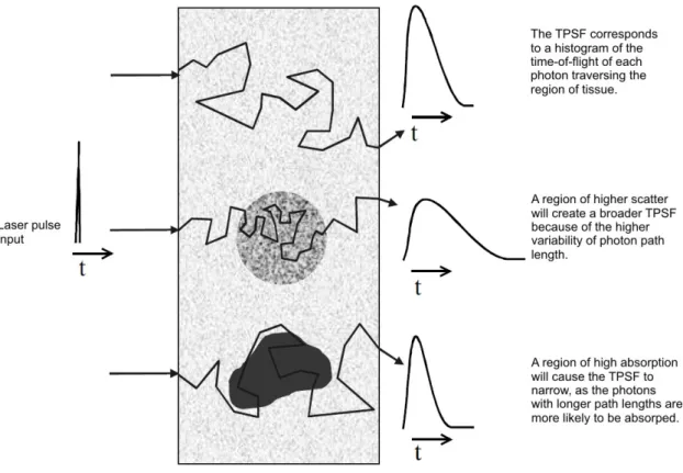
Time-resolved systems are the most complete systems out of the three, as the detection of the temporal distribution of photons as they leave the tissue provides more accurate information about tissue absorption and scattering information. They measure the tempo-ral point spread function (TPSF). The tissue is illuminated with a short duration (a few

picoseconds) pulse of NIR light. Due to the effect of scattering on the path of the pho-tons, this NIR pulse is broadened from a few picoseconds to several nanoseconds. The system measures the time of flight of the emerging photons and the information about the time taken for individual photons to traverse the volume of tissue from source to detec-tor is represented in a histogram - the TPSF. [17] Each TPSF corresponds to a distinct source-detector pair. This function contains more information than what is obtained from FR systems. When integrating a TPSF, one gets intensity information equivalent to a CW measurement; when doing the Fourier transform, one gets a continuous spectrum of am-plitude and phase shift data where each point is equivalent to a single frequency domain measurement (thus not depending on the computation of DPF); by applying the modified Beer-Lambert law, one gets information on absorption and scattering coefficients changes. Figure 1.11 illustrates how changes in optical properties of a volume of tissue will affect the resultant TPSF.

Figure 1.11: A summary of how the optical characteristics of tissue affect the TPSF recorded in time-domain imaging systems. Figure courtesy of J C Hebden.

Comparing with CW and FR systems, time-resolved have the advantage of increased penetration depth and a most accurate separation of absorption and scattering effects. On the other hand, the size of the instrument, its cost and the stability and cooling issues are the downside of time-resolved systems.

Time-resolved systems have been used in the past two decades to study a broad range of conditions. While it has been applied to the breast and to the muscle, most of its applications have been done on the brain. Optical imaging has been used to study neonatal

seizure, schizophrenia, and depression, and to map functions of the brain, such as the motor and visual cortex.

In general, NIR imaging equipment is portable, discreet and relatively robust to mo-tion artefact, enabling some motor experiments that can’t be conducted with other imaging techniques. Recently, other chromophores involved in brain activation, such as cytochrome-c-oxidase have been a research target.

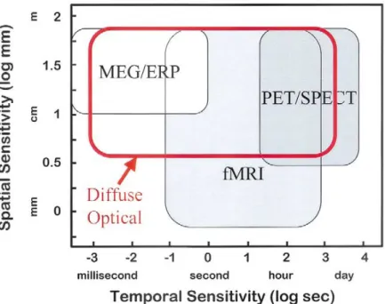
1.4.2.5 Comparison with other imaging techniques

The comparison of spatial and temporal sensitivity of positron emission tomography (PET), single positron emission computed tomography (SPECT), magnetoencephalog-raphy (MEG), functional magnetic resonance imaging (fMRI) and event-triggered EEG (also called event related potentials (ERP)s) is presented of figure 1.12.

It is clear that MEG and ERPs are strong in temporal sensitivity but relatively weak in terms of spatial sensitivity. In contrast, fMRI, PET and SPECT are stronger in spatial sensitivity but weak in terms of temporal resolution. DOI, in comparison, can provide excellent temporal sensitivity as well as reasonable spatial sensitivity. In contrast, fMRI, PET and SPECT are stronger in spatial sensitivity but weak in terms of temporal res-olution. When comparing with DOI, we see that DOI can provide excellent temporal sensitivity as well as reasonable spatial sensitivity. [33] This explains why the emphasis of research in medical imaging with DOI has moved away from the pursuit of high spatial resolution and towards functional imaging. Another growing research area is the coupling of optical imaging with other imaging techniques such as MRI, MEG and EEG.

Figure 1.12: Comparison of the spatial sensitivity and temporal sensitivity of six non- or minimally-invasive neuroimaging methods. [33]

Figure 1.13: MONSTIR, a 32-channel system designed for optical tomography of the newborn infant brain

Experiments with adults suggests that the characteristics of the vascular response mea-sured by NIRS are comparable to the blood oxygen level dependence (BOLD) response seen in fMRI. It is important to note that unlike fMRI BOLD, functional NIRS provides a separate measure of quantified changes in both HbO2 and HHb.

1.4.3

MONSTIR

The work described in this thesis was performed using a time-resolved tomography sys-tem available at the BORL at UCL. This device is called MONSTIR, it is the second generation system and is displayed in figure 1.13. It provides temporal measurements of photons transmitted diffusively through the tissue, enabling the reconstruction of internal distributions of absorption and scattering properties. It is the second version of a device that was designed to be portable, relatively robust to motion artefact and to continuously monitor premature babies’ brains for obtaining optical images at bedside. These babies are at an increased risk of suffering permanent brain damage due to dysfunction in cere-bral oxygenation. However, this version is still being studied and optimized before being used in a clinical environment. A schematic diagram is shown in figure 1.14.

The source of laser light is a Fianium supercontinuum laser. Supercontinuum light can be best described as ‘broad as a lamp, bright as a laser’. Incandescent and fluorescent lamps, such as those made from tungsten halogens, provide a very broad spectrum (400

Figure 1.14: Schematic functioning of MONSTIR. Figure courtesy of J C Hebden.

nm to 1700 nm) but the intensity is limited. Furthermore, as the light is not spatially coherent, coupling the light into a fibre would be challenging, resulting in a low-power, low-brightness source with mediocre beam quality. Lasers on the other hand have high spatial coherence and very high brightness, which enables optimum coupling to a fibre and outstanding single-mode beam quality. However, lasers are usually monochromatic, and thus if more than one wavelength is required extra lasers are necessary to cover a broad spectrum. A supercontinuum source bridges this gap, providing an ultrabroadband white-light spectrum but with the brightness of a laser and as high energy picosecond pulses. Figure 1.16 shows the broad emission spectrum that can be achieved. [26] The supercontinuum laser is controlled by a computer where it is possible to select up to four wavelengths within 600 and 1100 nm to be emitted in the same experiment.

This selection is performed by the acousto-optical tunable filters (AOTF)s, which functions as an electronically tunable bandpass filter to simultaneously modulate the in-tensity and wavelength of laser light. Devices of this type rely on a crystal whose optical properties vary upon interaction with an acoustic wave. Changes in the acoustic frequency applied to the AOTF transducer alter the diffraction properties of the crystal to control the transmitted wavelength. Changes in the amplitude level applied to the transducer con-trol, the transmitted light intensity level. In short, AOTFs enable very rapid intensity and wavelength tuning (several µ seconds), limited only by the acoustic transit time across the crystal. [14] The light path through the two AOTFs is described in figure 1.15.

A reference pulse is split off the laser beam with a beamsplitter and illuminates a fast photodiode. The resultant electronic pulses are sent to the time correlated single photon counting (TCSPC) unit and will be compared with the measured signal.

The main part of the laser beam goes through a neutral density filter that attenuates the light to the desired level - it is indicated in figure 1.14 as variable optical attenuator (VOA). The amount of light which can be coupled into the scalp is limited for safety reasons, and most NIR systems maintain an output intensity below that of the eye safety limit (10 W/m2for NIR wavelengths in continuous operation - British Standard EN 60825-1:2007).

Figure 1.16: Comparison of the output power of supercontinuum lasers, Helium-Neon lasers, Xenon lamps and superluminescent LEDs. [26]

[9] The laser beam then passes through an electronically controlled shutter and a beam splitter, and is coupled into a 1x32 fibre switch. The light is distributed into the 32 source fibre bundles. These optical fibres are held in contact with the surface of the interrogated object. The end of each source fibre is common to the end of a detector fibre, but while each source is illuminated sequentially (we say the source is moved over the object), all the detectors are simultaneously collecting the photons that exit the object. This co-axial arrangement of the source fibre within the detector bundle decreases the number of connectors to the interrogated structure. The photons then travel through the detector fibre bundles and are forwarded to the 32 photomultiplier tubes (PMT)s. However, since there is a large variation in source-detector fibre separation there is a correspondingly very large range of intensities of light emerging from the tissue surface and going to the PMTs. Due to the risk of saturating or damaging the PMTs, a set of 32 VOAs ensures that the light reaching the PMTs is not too intense. The PMTs amplify the current produced by the incident light, which then reaches the 32 independent TCSPC units. The TCSPC units measure the photon flight times and the delay between the measured signal and the reference one (received directly via the laser). Thus histograms of photon flight times (TPSFs) are gradually built and read out by the control PC. The full set of TPSFs - up to 1024 TPSFs when using 32 sources and 32 detectors - represents the raw data that is used for the reconstruction of absorption and scattering maps.

The process of image reconstruction is explored in section 1.5.

1.4.4

10-20 system

When setting up the experiment, the location of the optodes is done according to the 10-20 system, which is an internationally standardized system usually employed in EEG. This method is based on the relationship between the location of an electrode and the underly-ing area of cerebral cortex, and was developed to ensure standardized reproducibility so that a subject’s study could be compared over time, and subjects could be compared to each other. In this system, EEG electrodes are located on the surface of the scalp as shown in figure 1.17 (21 electrodes are shown, though a higher or lower number can be used). There are two reference points: the nasion, which is the indent between the forehead and the nose; and the inion, which is the bony lump on the midline at the back of the head. From these points, the electrode are located in the transverse and median planes, which are divided into 10% and 20% intervals. [20] Each site has a letter to identify the lobe (there is no central lobe but the "C" letter is used for identification purposes). Even num-bers (2,4,6,8) refer to electrode positions on the right hemisphere, whereas odd numnum-bers (1,3,5,7) refer to those on the left hemisphere. Letter "z" (zero) refers to the electrodes placed on the midline.

1.5

Image reconstruction

In time-resolved systems we perform a finite set of measurements of the light properties in order to reconstruct 2D or even 3D images of the distribution of internal scatterers and absorbers. The measured changes in intensity, phase and amplitude (datatypes extracted from the TPSFs) are caused by a change in the optical properties of the tissue. This change

Figure 1.17: The international 10-20 system seen from (A) left and (B) above the head. A = Ear lobe, C = central, Pg = nasopharyngeal, P = parietal, F = frontal, Fp = frontal polar, O = occipital. [20]

in the optical properties (absorption, scattering), which is what we want to know, is due to some activation in the neurons of the interrogated volume. The steps of optical imaging reconstruction are the modelling of light transport in tissue, the solving of a forward problem (which results in a sensitivity matrix) and the solving of an inverse problem.

The model of the photons behaviour in tissue relies on the diffusion equation derived from the radiative transport equation. If we have a model to predict the distribution of light in the interrogated object, what change in the data (TPSF) do we get for a given change in the internal optical properties ?

This is the forward problem, which consists in simulating the measurements from the model and generating a sensitivity matrix J that relates the measurements to the internal optical properties. In order to solve forward problems for complex geometries, numerical modelling techniques such as finite-element method (FEM) are needed.

∆I = J ∗ ∆x (1.12) The linear equation (1.12) assumes that any variation in optical properties is small and is related linearly to the change in measurement. It represents the following: we measure the change ∆I in a specific channel, we modelled J and we want to know ∆x which is the change in optical properties of the correspondent tissue. Therefore J has to be inverted, and this consists in the inverse problem of optical imaging reconstruction.

The software Temporal Optical Absorption and Scattering Tomography (TOAST) de-veloped at UCL was used for the FEM and to produce the sensitivity matrix (i.e. model where the light has gone and how a change in optical properties affects the change in intensity or mean time or whatever).

Also, in order to increase image quality, the practical aspects of the experiment need to be optimized, such as the maximisation of the number of source-detector pairs (channels) per unit surface area; the arrangement of these channels so that the number of channels sampling a given volume of tissue is optimum maximize the variety of source-detector

separations to increase the range of depths for which meaningful images can be recon-structed. [9]

1.6

Wavelength choice

The choice of wavelengths to use for NIR studies is a complex one. As explained in sec-tion 1.2.2.2, the NIR window used for tissue optics is bounded roughly between 650 and 900 nm. At lower wavelengths, absorption by haemoglobin limits penetration in tissue, while at higher wavelengths, absorption by water dominates. NIRS studies of the brain have typically employed wavelengths either side of the isobestic point of haemoglobin (800 nm), where the specific extinction coefficients of HbO and HHb are equal. The actual wavelengths used for a given study are usually determined for the particular exper-iment and are often dictated by the availability of appropriate light sources. [10] However, this choice shouldn’t be arbitrary, as events such as cross-talk and low separation between absorption and scattering will not only reduce the quantitative accuracy with which the changes can be determined but also change the shape of the timecourse of the signal. [35] Recently, Yamashita et al. (2001), Strangman et al. (2003) and Uludag et al. (2004) have shown experimentally and theoretically that a pair of wavelengths at 660-760 nm and 830 nm provides superior separation between HHb and HbO than the more commonly used 780 and 830 nm.

S. Lloyd-Fox et al. (2010) reviewed 36 experiments from which 27 used 830 nm as one of the wavelengths - others were very close to this value, such as 825 and 828 nm. From these 27 experiments, 17 used a second wavelength equal or superior to 780 while the other 8 turned to wavelengths equal or lower than 760 nm. Looking at the temporal distribution of the experiments, they were all published since 1998 but it is only after 2004 (that is, between one and four years after the publication of the papers mentioned above) that wavelengths below 760 nm started to be used, demonstrating the impact of this kind of wavelength analysis. In the same S. Lloyd-Fox et al. review, of the 6 experiments using 4 wavelengths, the wavelengths were 775 nm, between 805 and 825 nm, 850 nm and between 905 and 910 nm.

Correia et al. (2010) did a systematic evaluation of the optimal wavelengths for NIR imaging to determine the wavelengths with the least influence of noise, the maximisation of absorption and scattering separation and sampling of the same volume of tissue. When looking for a combination of four wavelengths, these three conditions led to the choice 680 ± 5nm, 715 ± 14nm, 733 ± 7nm and 828 ± 9nm.

The experiment

2.1

Goal of the experiment

The present chapter describes the experiment that was performed to empirically deter-mine the best set of 4 wavelengths to use when imaging the brain. This experiment was designed considering the performance characteristics of MONSTIR (the optical imaging device employed), which are described in section 1.4.3. In short, we require at least two measurements because we wish to perform differential imaging, and we use at least two wavelengths because we study two chromophores (in this case, oxyhaemoglobin and de-oxyhaemoglobin). MONSTIR brings the possibility of recording data at 4 wavelengths simultaneously. This can prove to be useful for several reasons, such as because over-sampling is always useful and because we get to study other chromophores such as the background chromophores. In fact, fat and water concentrations are usually wrongly as-sumed to be uniform throughout the tissue volume, although they are not expected to vary with time. The part of the brain imaged for this wavelength analysis is the motor cortex, as it is close to the scalp (i.e. within reach of the optical measurement depth) and its stimulus is easy to perform.

2.2

Array design and construction

The main concerns when designing an array are the size of the area of the head that we need to cover, the number of fibres needed, the distance between the fibres, and the comfort for the wearer of the array. Because we want to image the brain of an adult, it is not feasible to perform full-brain tomography of the adult brain because this requires measurements across the entire width of the head, which not produce measurable signals. Instead, optical topography is performed, which doesn’t preclude 3D images from being reconstructed. The experiment was designed to measure activity in the motor cortex of the left hemisphere, over a region about 7 or 8 cm in length. Since the imaged area are the tissues located immediately below the array, the dimensions of the array should similar to the dimensions of the area of interest. The minimum distance between two adjacent fibres should be at least 2 cm to prevent too much light from being detected and damaging the PMTs. Knowing this minimum distance, it is important to maximise the number of channels per unit surface area.

Figure 2.1: Array design. C3 is the center of the motor cortex. Red dots are the source fibres (which also work as detectors) and blue dots are the detectors. The distance between fibres is in millimetres.

The array employed for this experiment had 9 channels and is illustrated in figure 2.1. The smallest source-detector distance is 27.50 mm and the largest is 73.15 mm. As explained in the end of section 1.5, this variety of source-detector separations is important. Using the 10-20 system, the center of the motor cortex is C3 (see figure 1.17A). This point is the center of the fibres arrangement and is the reference to place the array on the head. The source fibres were positioned both above and under C3, making the array vertically symmetric. As planned, when tracing the path between each source and every detector, we see that the same volume of tissue is sampled more than once by different channels.

The array is based on a commercial EEG cap. It is cheap, comfortable and adaptable for any adult subject; the main points of the 10-20 system are marked on the cap. With the cap on the subject, the dots of figure 2.1 were marked on the cap and then perforated -see figure 2.2A. Due to the shape of the fibre tips, it was necessary to design a customised connector to secure the MONSTIR optical fibres on to the EEG cap, and ensure they remain in the correct position. Thus 9 connectors, as shown in figure 2.3, were 3D printed in two parts. The printed material was optically transparent and therefore the connectors were painted black to prevent light leakage. A prism was inserted into each connector to defect the light 90 degrees on the head surface. This prism is seen on figure 2.3 and was glued to the sockets. After gluing the halves together, the socket has one end where the fibre fits, and an other circular end that clamps the cap tissue. A small hole was drilled on the side of the socket so that a screw would press the fibre inside the socket.

2.3

Experiment design

Since we are doing difference imaging, it is necessary to measure brain activity during rest and during stimulus. The stimulus consists of a simple finger-tapping task of touching the

thumb and each of the fingers of the right hand (which is contralateral to the side of the head studied) sequentially. This task is repeated several times (i.e., it is interrupted with pauses) while maintaining the same conditions in order to improve signal-to-noise ratio, but is also repeated using different sets of wavelengths so that the purpose of the experiment is fulfilled. Figure 2.4 illustrates one single acquisition or one run of the experiment and will be described in the following paragraphs.

.

Figure 2.4: Temporal scheme of one acquisition of the experiment

In the perspective of the subject, one run of the experiment consists of 10 seconds of rest followed by approximately 15 seconds of finger-tapping and 20 seconds rest. The transitions from rest to movement and movement to rest are signalled by the person who is responsible for the experiment. The several runs consist of a cyclic repetition of the process described, therefore the two rest stages get merged and the subject ends up resting for approximately 30 seconds.

The rest data is acquired during the 10 seconds of the first rest stage. Then the subject starts finger-tapping and no data is acquired during approximately 5 seconds. This gives time for the vascular response to develop and reach its maximum, but also allows the person performing the experiment to save the rest data that was just acquired. Finger-tapping data is then acquired for 10 seconds, followed by a pause in finger-Finger-tapping and in data acquisition. The second stage of rest is necessary for saving the stimulus data and is crucial for the vascular response to go back to baseline so that it can be newly acquired in the next repetition. Between 0 and 5 seconds of rest are randomly added to this period so that the delay time between acquisitions varies every time. This jiggering thus prevents natural periodic oscillations in the chromophores being interpreted as an evoked activation.

The full data acquisition consists on the repetition of this single acquisition with some changes made to the sources’ order and the wavelengths used. The array of fibre bundles covering the motor cortex area has nine bundles, and each of them can work both as a source and as a detector. The chosen sources illuminate one at a time while all the remaining fibres serve as detectors. When one fibre is being illuminated (i.e. serving as a source) its corresponding detector is blocked by the VOA, to prevent the PMT being over-exposed (and potentially damaged) by the large amount of back-reflected light. Therefore if we are using nine bundles, the number of detectors working simultaneously is eight. Since the sources work only one at a time, the number of sources used is the main factor