Supermarket site assessment and the importance of spatial analysis data

WORKING PAPER SERIES

Universidade dos Açores

CEEAplA WP No. 07/2006

Supermarket Site Assessment and the

Importance of Spatial Analysis Data

Armando Mendes

Margarida G.M.S. Cardoso

Rui Carvalho Oliveira

June 2006

Supermarket Site Assessment and the

Importance of Spatial Analysis Data

Armando Mendes

Universidade dos Açores (DM)

e CEEAplA

Margarida G.M.S. Cardoso

ISCTE (Departamento de Métodos Quantitativos)

Rui Carvalho Oliveira

CESUR (Institituto Superior Técnico)

Working Paper n.º 07/2006

Junho de 2006

CEEAplA Working Paper n.º 07/2006

Junho de 2006

RESUMO/ABSTRACT

Supermarket Site Assessment and the

Importance of Spatial Analysis Data

This work is part of a dissertation that addresses the supermarket site

assessment problem. We propose a 3-steps method for stores’ site evaluation.

(The 1st step yields the constitution of analogue groups of existent

supermarkets, using a clustering procedure. On the 2

nd

_{step we use}

classification trees to classify new stores into specific analogue groups. Finally,

on the 3

rd

step, we build a linear regression model to forecast new sites’ sales,

based on several predictor variables, including dummy variables referred to

analogue groups).

In order to deal with demographic and competition data related to each

supermarket, we use neighbourhood delimitation techniques. Three alternative

delimitation techniques and twoaggregation procedures are compared. Results

are evaluated based on the proportion of sales turnover variance that the

alternative predictors are able to explain. (As a result, we select one

aggregation procedure, although we conclude that none of the delimitation

models: shortest path polygons and multiplicative weighted Voronoi diagrams,

first and second order, present similar performance).

Finally, we compare the relative importance of spatial data predictors in site

assessment evaluation, using Dominance Analysis. As a result, the relevance of

spatial analysis predictors clearly emerges being only dominated by the “trade

area”.

Keywords: Supermarket site assessment; analogue discriminant site selection;

multiplicative weighted Voronoi diagrams; dominance analysis.

Armando Mendes

Departamento de Matemática

Universidade dos Açores

Rua da Mãe de Deus, 58

9501-801 Ponta Delgada

Margarida G.M.S. Cardoso

Departamento de Métodos Quantitativos

ISCTE – Escola de Gestão

Av. Das Forças Armadas

1649-026 Lisboa

Rui Carvalho Oliveira

CESUR – Instituto Superior Técnico

Av. Rovisco Pais

Supermarket Site Assessment and the

Importance of Spatial Analysis Data

Armando B. Mendes

1

CEEAplA and Mathematical Department, Azores University, R. da Mãe de Deus, 9501-801 Ponta Delgada, Portugal

amendes@notes.uac.pt

Margarida G.M.S. Cardoso

Department of Quantitative Methods, Business School ISCTE, Av. das Forças Armadas, 1649-026 Lisboa, Portugal

margarida.cardoso@iscte.pt

Rui Carvalho Oliveira

CESUR, Instituto Superior Técnico, Lisbon Technical University Av. Rovisco Pais, 1049-001 Lisboa, Portugal

roliv@ist.utl.pt

Abstract:

This work is part of a dissertation that addresses the supermarket site assessment problem.

We propose a 3-steps method for stores’ site evaluation. (The 1st step yields the constitution

of analogue groups of existent supermarkets, using a clustering procedure. On the 2nd step

we use classification trees to classify new stores into specific analogue groups. Finally, on

the 3rd step, we build a linear regression model to forecast new sites’ sales, based on several

predictor variables, including dummy variables referred to analogue groups).

In order to deal with demographic and competition data related to each supermarket, we use neighbourhood delimitation techniques. Three alternative delimitation techniques and two aggregation procedures are compared. Results are evaluated based on the proportion of sales turnover variance that the alternative predictors are able to explain. (As a result, we select one aggregation procedure, although we conclude that none of the delimitation models: shortest path polygons and multiplicative weighted Voronoi diagrams, first and second order, present similar performance).

Finally, we compare the relative importance of spatial data predictors in site assessment evaluation, using Dominance Analysis. As a result, the relevance of spatial analysis predictors clearly emerges being only dominated by the “trade area”.

Keywords:

Supermarket site assessment; analogue discriminant site selection; multiplicative weighted Voronoi diagrams; dominance analysis.

1

Corresponding author: R. da Mãe de Deus, 9501-801 Ponta Delgada, Portugal. amendes@notes.uac.pt. Telephone +351 296 65 00 73, Fax: +351 296 65 00 72.

1. Introduction

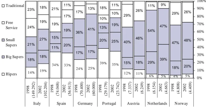
The importance of the retail sector in Europe is well established as one of the biggest employers and with a global value of sales turnover in the 15 countries of the European Union of 111.5 billions euros in 2000. On the other hand, not specialized stores as supermarkets and hypermarkets are responsible for 85.4% of the total sales (Eurostat, 2003). In spite of the great heterogeneity observed across the different European countries several of these countries as Germany, France, Spain and Italy suffered a similar evolution (see Figure 1). After an unprecedented period of hypermarkets growth, since the late 1970s, both in number and market share, it is now clear that hypermarket activity has slowed down significantly on behalf of the small to medium supermarkets (chain outlets including discount and hard discount chains) that nowadays present a larger dynamism (Eurostat, 2001).

Figure 1 – Market share for 1998 and 2002 by food outlet type in several European Countries.

(Source: A.C. Nielsen Portugal. Total number of stores in brackets)

5% 4% 5% 6% 11% 12% 35% 39% 25% 24% 33% 34% 19% 14% 20% 18% 39% 29% 18% 15% 25% 20% 17% 17% 20% 11% 18% 18% 48% 47% 47% 54% 46% 40% 19% 13% 41% 36% 19% 15% 27% 21% 26% 29% 9% 11% 26% 29% 10% 10% 13% 17% 17% 19% 19% 24% 11% 18% 11% 21% 18% 23% 0% 10% 20% 30% 40% 50% 60% 70% 80% 90% 100% 20 02 (4 .409 ) 19 98 (4 .808 ) 20 02 (4 .663 ) 19 98 (6 .154 ) 20 02 (6 .249 ) 19 98 (7 .337 ) 2002 (23. 742 ) 1998 (29. 179 ) 2002 (60. 000 ) 1998 (70. 400 ) 2002 (56. 913 ) 1998 (74. 048 ) 20 02 (102. 204 ) 19 98 (149. 292 ) Norway Netherlands Austria Portugal Germany Sp ain Italy T raditional Free Service Small Sup ers Big Sup ers

Hip ers

Several authors (e.g. Birkin et al., 2002, Dawson, 2000, and Seth and Randall, 1999) identify such factors as increasing consumer mobility, increasing electronic commerce, changing household size, concentration of market power, home market saturation, and changes in planning legislation to justify the new trends in retailing. In Portugal market share data shows that since 1996 the supermarkets are the only ones to grow simultaneously in the number of

outlets and in the volume of sales and, consequently, to increase the market share from 28 to 34% in the A.C. Nielsen universe. In 1997 the supermarkets reached the leadership and consolidated its expansion strategy. More demanding consumers force the retail groups to invest in smaller stores, and so in a proximity and quality of goods and services strategy. Several authors agree that the future of the proximity small to medium supermarket looks promising. Birkin et al. (2002) considers that in the near future we should anticipate an important growth (or return) of this type of stores in Europe, mainly by means of franchising. In other hand, Dawson (2000) integrates this growth of smaller grocery stores in a multi-format strategy used by the largest European retail groups, already very common in the United States of America.

But, the pressures that the grocery chain supermarkets face are such that the location decisions cannot be neglectful. The investment in smaller stores has a longer run return as well as smaller economies of scale, which forces careful decision-making (McGoldrick, 2000, Salvaneschi, 1996). The stores represent locations where significant volumes of capital are invested and, once taken, the location decisions are difficult to change. In this way, companies cannot continue to take decisions with relation to marketing mix’s fourth P (of place) based on “gut feels” (Gilbert, 2002). Works like the ones presented by Pioch and Byrom (2004) and Jones et al. (2003) confirm the need for a good location, especially in standardized services with less personalized attendance, as it is the case of supermarket multi-store chains.

In this paper a methodology for new store supermarket site assessment is presented based in data analysis methods and using spatial analysis data. The 3-steps method comprises a 1st step which yields the constitution of analogue groups of existent supermarkets, using a clustering procedure. On the 2nd step classification trees are used to classify new stores into specific analogue groups. Finally, on the 3rd step, we build a linear regression model to forecast new sites’ sales, based on several predictor variables, including dummy variables referred to analogue groups.

In all these steps many variable types are used for model estimation and validation. These variables were collected using surveys, a mystery shopping program, competition location, and georeferenced demographic data. To include this last type of data, in a point location study, influence areas are delimited and aggregation procedures defined. Those combinations of the influence area delimitation models and aggregation procedures are used for predictor calculation and evaluated based on the proportion of sales turnover variance that they are able to explain. In order to assess the relative importance of spatial analysis predictors in contrast to all other types, a dominance analysis study is presented.

2. GIS and Influence Area Delimitation Models

The use of Geographical Information Systems (GIS) in support of location decisions presents several advantages. The power of GIS applications resides in its capacity to integrate information related to geographical position, to manipulate many kinds of attributes, to perform space analyses, and easily produce thematic maps and other data visualizations (Church, 2002). In this way, GIS applications make possible the spatial analysis of locations integrating demographic variables, trip extent, real state data, and competition as well as customers’ locations. Other advantages are related with the easiness of modelling accessibilities and the growing readiness of road networks and geodemographic data.

Although some analysts continue to delineate influence areas by simple direct observation of the customers' distribution in the space of analogue supermarkets, the presence of GIS software in the companies has been changing this scenario. Among the simplest methods using GIS, are buffers or circumferences with an appropriate radius and polygons defined by shortest path algorithms (SPA) over a street network (e.g. Boots, 2002, Birkin et al., 2002;

McMullin, 2000). In this article, we also suggest the use of multiplicative weighted Voronoi diagrams (MWVD), first and second order. The latter model allows, simultaneously, the

integration of the supermarket attractivity and the competition in the store proximities (Boots and South, 1997).

Although the Voronoi diagrams are traditionally attributed to pioneer mathematicians as Georges Voronoï (1908) ou Peter Gustav Lejeune Dirichlet (1850), they have been discovered and rediscovered several times in science history. Actually, they can be found in the part III of the Principia Philosophiae and in the treatment of cosmic fragmentation of René Descartes, both published in 1644. As examples of Voronoi diagram rediscover Okabe

et al. (2000) mention many cases in domains as crystallography, meteorology, geography,

and ecology. At present, there are an impressive number of published works on algorithms and applications (see for example Okabe et al., 2000 or Berg et al., 2000). In what refers to multiplicative Voronoi diagrams in the characterization of proximity elements of a group of points in the space corresponding to grocery supermarkets, Boots and South (1997) present a very complete work. Although older references can be found (see for instance Shieh, 1985), in the mentioned paper an integrated vision on the theme is presented, using Voronoi diagrams for descriptive and prescriptive proposes.

In this application the Voronoi diagrams are used in the characterization of the proximity of a generator group of

P = {p

1

, p

2

,…, p

n

}

points in the space (with

2 ≤ n < ∞

), known as the point

generator group, corresponding to supermarkets. The diagram is defined as a space partition where each point of the space associates to the closest element of the generator group. If the proximity function is the Euclidian distance, the partition will result in a series of

n

polygons (Voronoi polygons) and it takes the name of Ordinary Voronoi Diagram (OVD) (Okabe et al., 2000). Each polygon (

V(p

j

)

) generated by point

p

jwith coordinates

x

j is defined

by: } , : { ) (p x x x x x k j P V _j = − _j ≤ − _k ∀ ≠ ∈ (1)

where

k

is, in turn, all other elements of the generator group. The set of all polygons

V =

{V(p ), V(p ), …, V(p ), …, V(p )}

1 2 j n compose an Ordinary Voronoi Diagram. Noticeably

V(p )

j

contains all the points closest to

p

j than to any other element of the generator group.

equally attractive for a potential customer. These are very simple models that can be approximately valid for similar stores in densely populated areas, without geographical barriers on foot trips and with homogeneous demographic and psychographic conditions (Berg et al., 2000).

Multiplicative Weighted Voronoi Diagrams (MWVD) are defined in a similar way,

associating to each point of the generating group a positive weight (

w

j) quantifying its

attractivity, and being a function of the supermarket’s characteristics and the site. The distance function (

d

wj) is given, in this case, by:

0

,

)

/

1

(

)

,

(

_j

=

_j

⋅

−

_{j j}

>

w

p

p

w

x

x

w

d

j ₍₂₎

Thus, each MWVD is defined by:

}

),

,

(

)

,

(

:

{

)

(

p

x

d

p

p

d

p

p

k

j

P

V

_{j w j w k} k j

≤

∀

≠

∈

=

(3)

In this paper preference is given to multiplicative Voronoi diagrams over others as the additively weighted Voronoi diagrams (see Okabe et al., 2000), since they can be regarded as simple space interaction models. Modelling the supply and demand for food, representing the supply by the point generator group, the Voronoi polygon associated to each element of the resulting partition is interpreted as the influence area of the respective generating element, assigning to this area all the points in the space that maximize the utility function:

0

and

/

−

>

=

α

α

j i j ij

A

x

x

U

(4)

This utility function is a particular case of the following expression for the generic utility function linking the supply points (j), in this case supermarkets, to demand points (i), in this case potential costumers or points in the space:

j i ij ij j ij

A

d

d

x

x

U

=

−

≥

=

−

,

0

,

and

α

β

β α (5)

where A j is the attractivity of the supply point j, d ijis any kind of distance, travel time or trip

cost between the supply point i and the demand j, and α,

β

are parameters. Gravitational models are space interaction models derived from a ratio between the utility function (5) for a

supply point over the total of all utilities for the competing supply points. These models are used as an estimate of the market share of the supply point

j

or as an impact model. The MWVD’s use the same utility function to accomplish the space partition since the weight corresponds to the store attractivity power αand

β is fixed to one. And so, the MWVD

assume that the customers value the proximity in the choice of the store (as in the OVD) but also introduce the attractivity concept. Thus, the store choice process depends on a trade-off between the proximity and the store attractivity, as in the gravitational models.

These models can still be extended if we consider that customers can frequent

k > 1

supermarkets or generating points, simultaneously. The Order-

k

Multiplicative Weighted Voronoi diagrams (OkMWVD) come from evidence found in the surveys where a large

majority of costumers declare to simultaneously frequent other stores, mainly hypermarkets and superstores. Consider all the subsets of

k

stores (generator points) among the

n

existent:

P = {P (k), …, P (k), …, P (k)}

1 i l with

l= C

n k. Consider also one of these groups

P (k)

= {p , p , …, p

i i1 i2 ik

}

, so the OkMWVD (

V(P (k

i

)

) is:

)}

(

\

),

,

(

{

min

)}

(

),

,

(

{

max

:

{

))

(

(

P

k

x

d

p

p

p

P

k

d

p

p

p

P

P

k

V

_{i p w j j i p w r r i} r r j j

∈

≤

∈

=

(6)

which relates any point of the space with the

k

near by more attractive stores.

Several assumptions are enumerated by Okabe and Suzuki (1997) wich must be keep in mind when these models are applied to a a particular location problem:

•

n

competing stores located in the same planar and finite region;

• all clients inside a Voronoi Polygon endorse only one store (in MWVD), or

k

stores (in OkMWVD) to probabilities proportional to the ratio of utilities;

• the utility function

U

ij for the

j

store and

i

costumer is an inverse function of the Euclidian

distance between the two and a direct function of the store attractivity;

• the weight function

w

j (

> 0

) is supposed to be derived from variables related to the site

and the particular store as store dimension, accessibilities, etc..

Several of these assumptions are not considered in shortest path polygons. For instance, non planar areas can be modelled by distinct average velocities in some street fragments.

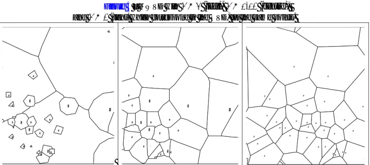
But, shortest path algorithms also have disadvantages. They are adequate for car trips but unsatisfactory for walking trips, where accessibility networks are difficult or impossible to define. In surveys more than 60% of the shopping trips were walking trips, and in some supermarket segments this percentage is much higher. Shortest path polygons also don’t include any competition mechanism, and polygons from competitive shops frequently overlap, as seen in Figure 2.

An intermediate situation between the mutual disjunctive tessellation in the MWVD and the strong overlap in shortest path polygons are the O2MWVD. These Voronoi polygons define influence areas as the spatial union among all polygons allocated to a particular supermarket, and result in the overlap with other near by stores as is evident from Figure 2. The O2MWVD also present the advantage of frequently defining larger influence areas over the MWVD that, some times, define too small polygons.

As none of the mentioned models for influence area definition appear to be theoretically superior to the others, all of than are considered and compared in this paper.

Figure 2 – 2 min. shortest path polygons (left) and multiplicative weighted Voronoi

diagrams, first (centre) and second order (right), examples. (Stores as points and influence areas in grey. First two maps also show the road network and the third the first order MWVD).

# # # # # # # # # _# # # # # # # # # # # # # # _# # # # # # # # # # # # # # _# # # # # # # # # # # # # # # # # # # # # # # # # # # # # # # # # # # # # # # # # # # # # # # # # # # # # # # # # # # A B C D E F (A,B) (E,A) (A,F) (B,A) (D,A) # # # # # # # # # A B C D E F (A,B) (E,A) (A,F) (B,A) (D,A)

3. Supermarkets’ Site Assessment Data

3.1. Empirical framework

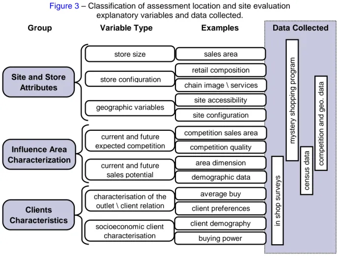
Several attributes are relevant for the problem of supermarket site assessment. A data framework is suggested in Figure 3 where the data is classified in three groups namely: location and supermarket attributes, influence area characterization and clients’ characteristics. This empirical framework, is intended for store and site evaluation of small to medium dimension supermarkets belonging to a retail chain, and is based in the authors’ experience and in an extensive literature review.

Figure 3 – Classification of assessment location and site evaluation

explanatory variables and data collected.

Group Variable Type Examples Data Collected

Site and Store Attributes

geographic variables store size

store configuration

current and future expected competition

retail composition chain image \ services

site accessibility site configuration

demographic data area dimension competition sales area

competition quality client demography buying power average buy client preferences in s hop s u rv ey s c o m pet it ion and geo . dat a m y s ter y s hop pin g pr ogr am c ens us da ta sales area Influence Area Characterization Clients Characteristics

current and future sales potential characterisation of the

outlet \ client relation socioeconomic client

characterisation

From Figure 3 the theoretical importance of demographic data (census data) and other spatial analysis data (competitive and geographical data) is clearly marked. Only the store size, store configuration and clients’ characteristics are not covered by this type of data. In fact, clients’ characteristics are the most relevant for chain supermarkets, as the store configuration, and in some way the trade area, tends to be very similar inside a chain. In

spite of their relevance in store clustering and characterization, the clients’ characteristics can not be used in new store sales predictions, as they are collected by surveys.

To cover all the relevant aspects, a large number of variables were collected in order to account for the diversity of attributes that may influence supermarkets performance evaluation, and so, should be included in model estimation. The data collection phase was very time consuming and concerned several different techniques enumerated and explained in a previous work (Mendes and Cardoso, 2005). Of the fusion of all data collection procedures, a total of several hundred variables were obtained, measured in all kind of scales.

3.2. Influence Area Characterization

In these work, quantitative variables from the national geographical census 2001 data are available in several disaggregation degrees, and ready to use in a Geographical Information System. These data is georeferenced to polygon shapes, known as statistical sections, and must be intersected with influence areas polygons. In this paper, we propose two criteria for aggregation of the demographic polygons in influence areas resulting from the geospatial intersection.

To any of the mentioned influence area delimitation models to be applied several parameters must be estimated. For this propose the 80% empirical rule is, when possible, employed. This rule considers that approximately 80% of the costumer’s trip origins must be inside the influence area polygon (Salvaneschi, 1996). In this particular work, the same parameter values must be applied to all shops, meaning that some of the shops will obey the 80% rule and some will not. The methodology applied maximized the number of shops obeying the rule as a starting point and them the areas were evaluated and adjusted by location experts. The experts are marketing analysts’ specialised in food retail store location, working with the supermarket chain since its origin and being responsible for all location and performance studies. For the shortest path polygons, and having a street network and estimates for car mean velocities, the only parameter consists on the trip limit time. Using the 80% rule and in

agreement with the location specialists, the 2 ½ minutes value was adopted, which corresponds to approximately 10 minutes in walking trips.

For influence area delimitation by Voronoi diagrams a data base with the location of more than 600 grocery outlets in Portugal was necessary for the model estimation. This data was collected in coordination with the mystery shopping program and by recording GPS coordinates outside the store door. The scale parameter α, from equation (4), was estimated in a similar way, leading to a square root function. It should be noticed that the diagrams are highly sensitive to variations in this parameter, as very small variations lead to very deformed diagrams with big areas for the points with higher weights (α's bigger values) or it tend to OVD for lower values (see Figure 4).

Figure 4 – MWVD with α

= 2 (left),

α

= 1/10 (centre)

,

and α

= 0

(right) which correspond to the OVD, for the same points.

# S # S # S #S # S # S # S #S # S # S #S #S#S # S # S # S # S # S # S # S # S # S # S # S #S # S # S # S #S # S # S #S #S#S # S # S # S # S # S # S # S # S # S # S # S #S # S # S # S #S # S # S #S #S#S # S # S # S # S # S # S # S # S # S # S # S #S # S # S # S #S # S # S #S #S#S # S # S # S # S # S # S # S # S # # # # # # # # # # # # # # # _# # # # # # # ## # # # # # # # # # # # # # # # # # # # # # # # _# # # # # # # ## # # # # # # # #

For the store attraction function a linear regression method was used, using annual sales for the supermarket, as dependent variable, and explanatory variables as “trade area”, “number of years in operation” and dummy variables for the classification of the location as “city centre”, and the chain insignia. The obtained regression just explains 48% of the sales variability, what is not surprising given the limited number of explanatory variables available. For the aggregation of the polygons resulting from the intersection between the administrative limits of the statistical sections with associated demographic data, and the

influence area polygons, two different methods can be used. Authors as Cowen et al. (2000) and McMullin (2000) use the fraction of the statistical section covered by the influence area as a weight in a weighted average, as indicated in the equation (7). This procedure implies a uniform distribution of the data variable in the statistical section.

⎟⎟

⎠

⎞

⎜⎜

⎝

⎛

×

∑

=

related

variable

section

l

statistica

area

section

l

statistica

total

area

influence

by the

covered

area

section

l

statistica

1

i

i

i

m i ₍₇₎

Another available alternative consists of using the same weight in an inclusion decision rule for the statistical section. In this work, the 50% limit value is used to include statistical sections with higher fractions of area covered, and to exclude sections with lower fractions. This model has the disadvantage of distorting the original influence areas (compare shaded areas with influence area polygons in Figure 2), and the major advantage of adjusting the boundaries of the influence area to the boundaries of the statistical sections, what can be more appropriate as the statistical sections are defined by the National Statistics Institute considering geographical barriers.

From this aggregated data, variables as percentages of totals and densities per hectare are also calculated. For the Voronoi diagrams, a store is considered competition if it shares borders with the supermarket, and for the shortest path algorithms all the stores inside the polygon are considered competition. This analysis allow the calculation of competition variables as “sum of trade areas from competitors”, “sum of competition trade areas weighted by the inverse of shortest path distances”, “number of hypermarkets up to 15 minutes” or “area of Voronoi polygon”.

With the objective of comparing the different techniques used for the present case of chain grocery supermarkets, linear regressions are used using as explanatory all continuous variables resulting from the spatial analysis, calculated by combining the particular influence area delimitation model and aggregation procedure. The dependent variable used is the annual sales per unit of trade area. The best models as evaluated by adjusted squared multiple correlation coefficient values as presented in Table 1. From this table the adjusted R2 values are relatively low, what confirms the need for all the other data collected and for

the 3-steps method used. Nevertheless, all the models are significant by the F test to the 1% level.

Table 1 – Adjusted R2 for explanatory regressions of the annual sales per trade area1.

(The sign of the estimated coefficients is negative for the underlined variables). AGGREGATION PROCEDURE

DELIMITATION

MODEL _{WEIGHTED AVERAGE DECISION RULE}

Shortest Path Algorithm

Adjusted R2 = 52 % (“Number of non classical

households”, “Number of residents with less then 5 years old”,

“Percentage of families with at least two children or grandchildren not married”)

Adjusted R2 = 65 %

(“Number of classical families with children less then 5 years old”, “Percentage of non classical households”, “Percentage of woman with more than 65 years old”, “Density of buildings built between 1996 and 2001”)

Order 1 MWVD

Adjusted R2 = 59 %

(“Percentage of non classical households”, “Percentage of

resident individuals employed in the first and second economic sectors, “Number of buildings with 1 or 2 floors”, “Density of owned classical households”)

Adjusted R2 = 66%

(”Density of residents with more than 65 years old”,

”Percentage of individuals without any economic activity”, ”Number of classical buildings”)

Order 2 MWVD

Adjusted R2 = 53%

(“Percentage of non classical households”, “Percentage of woman between 10 and 24 years old”, “Percentage of families with at least two children or grandchildren not married”, “Percentage of

individuals working in the residential council”, “Number of buildings with more than 5 floors”)

Adjusted R2 = 67%

(“Percentage of non classical households”,

”Density of buildings built between 1996 and 2001”, ”Percentage of individuals working in the residential council”)

1

Linear Regressions by the stepwise method using 5% and 10% test F in and out parameters respectively. All the models are significant to 1% F test and all the estimated coefficients are significant by a 5% t test.

The different explanatory variables chosen indicate clearly that the values for the different variables are dependent on the calculation procedure. Although the results in the Table 1

refer to a small number of supermarkets and cannot be generalised, they indicate a clear preference of the aggregation method for the decision rule over the weighted average. On the contrary, in relation to the delimitation model the preference is not clear. In the following sections all the delimitation models are used in variable calculation but always combined with the decision rule aggregation procedure.

4. The 3-Steps Method for Site Evaluation

Site assessment or site evaluation can be defined as the assessment of potential locations and the selection of alternative site locations to maximize the sales of a supermarket chain (Lilien et al., 1992, Davies and Rogers, 1984). Site selection and evaluation comprises a set of different quantitative or non quantitative methodologies and techniques which include management judgment, analogue based models, multicriteria decision analysis, gravitational models, multiple regression analysis, discriminant analysis, supported with spatial data analysis, which are reviewed in Mendes and Themido (2004).

In order to evaluate supermarkets’ locations, by sales forecast for potential sites, we propose in this paper a 3-steps method, based in data analysis procedures, namely cluster analysis, classification trees and linear regression:

• step 1: Analogue groups of existent supermarkets are defined using a clustering procedure (Ward method) and expert knowledge.

• step 2: Classification tree models are used to provide the analogue groups’ characterization as well as propositional rules which allow the classification of new stores in one of the analogue groups.

• step 3: Linear regression models yield new site sales forecast based on several predictor variables including dummy variables for analogue groups encoding.

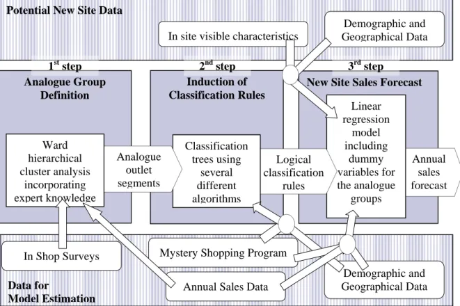
Figure 5 depicts the 3-steps method, data used for model estimation and data necessary for

new site annual sales forecast.

The data in Figure 3 is used for model estimation in the 3-steps data analysis approach. Not all data could be used in all the steps. For instance, the chosen method for analogue group definition used only metric variables. In spite of that, cluster characterization involved all the variables collected. Rule induction could use variables in any scale of measure, but because rules must include only variables that can be measured for potential new sites, all survey variables are discarded. Many of the mystery shopping attributes are also discarded as in store characteristics. Only in site visible characteristics are included as the available trade area, accessibilities, site visibility, nearby anchors, and other related with competition and influence area characterization.

Figure 5 – The 3-steps method for site evaluation.

Potential New Site Data

Demographic and Geographical Data In site visible characteristics

For the linear regression model, another restriction applies, as the non metric variables are difficult to include and hinders the process of variable selection by stepwise methods. In that context, as demographic and competition variables resulting for spatial analysis procedures, are almost all metric and easy to measure in new potential sites, they acquire a particular relevance for supermarket annual sales forecast.

4.1. Step 1 – The Definition of Supermarket’ Analogue Groups

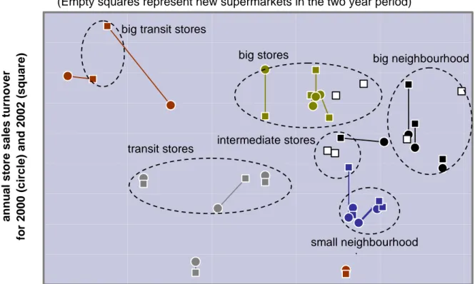
The step 1 involved the experts’ knowledge in the base clustering variables selection as well in the appreciation of the results from the successive hierarchical clustering procedures. The process was reinitialised several times with new base clustering variables when the clusters did not correspond to the expert’s expectations. In Figure 6 these clusters are depicted along with labels based on the characterization presented in Mendes and Cardoso (2005). The two supermarkets in the bottom of the chart are identified as outliers. Both had been previously picked up by retailing experts as these supermarkets had poor performances and dreadful

New Site Sales Forecast Analogue Group

Definition

Data for

Model Estimation

Annual Sales Data

Demographic and Geographical Data Mystery Shopping Program

Annual sales forecast Linear regression model including dummy variables for the analogue groups Induction of Classification Rules Logical classification rules Classification trees using several different algorithms Analogue outlet segments Ward hierarchical cluster analysis incorporating expert knowledge In Shop Surveys

locations. Depicted values refer to 2000 and 2002, as in these years in shop surveys were performed. In the latter year the inquiry was only done in some of the supermarkets, so a constant value are considered for plotting proposes. Empty squares represent six new supermarkets in 2002.

Figure 6 – Step 1 analogue supermarket clusters by the Ward method showing two years of data.

(Empty squares represent new supermarkets in the two year period)

percentage of exclusive trips in surveys

a nnua l s tore s a le s turnov e r fo r 2000 ( c ir cle) an d 2002 ( s q u ar e )

big transit stores

transit stores small neighbourhood t big neighbourhood big stores intermediate stores

Data used to characterize the six groups resulting from the clustering analysis is compared and relative importance of spatial analysis data evaluated by means of p-values for non-parametric Kruskal-Wallis tests. For variables without the order feature Chi-square tests are used. The Kruskal-Wallis test is considered very trustworthy and can be used for ordinal variables, in contrast to the parametric F test (see, for instance, Moutinho et al., 1988). In the p-value ranking, lower than 5%, all variable types and data collection methods are represented. In spite of this, the variables resulting from data analysis and classified as “influence area characterization” are, in this case, clearly the largest group with nine in the 15 variables with lower p-values.

4.2. Step 2 – Classification Trees and Rules Induced

In step 2 classification rules are induced. The objective is the identification of variables and propositional rules, in order to discriminate among the different groups of stores, for classification of new potential sites in an analogue group. Several logical propositional rules where induced from different algorithms, and the best rules are kept. The algorithms used are CART – Classification And Regression Trees (Breiman et al., 1984), CHAID – CHi-squared Automatic Interaction Detector (Kass, 1980, Biggs and Suen, 1991) and QUEST – Quick Unbiased Efficient Statistical Tree (Loh and Shih, 1997). The three algorithms can be distinguished by the homogenity measure used and the method to select the discriminant variable and respective partition condition.

For comparing and evaluating the different rules induced we propose the precision index, presented in expression (8). In this expression, the precision index for supermarket

j

is represented by

IP

j,

leaveOneOut

represents the estimate of the classification error by the

leave-one-out method for the model (

a

), the

%hits

the “hits percentage in the leaf” regarding the propositional rule (

a

r) and

%group

the “percentage of stores of the group in the leaf” for

the same rule.

(

₋

)

β_×

(

α _× −α

)

= 1

% %

1 _{a ar ar}

j leaveOneOut hits group

IP

, 0 ≤

α

≤ 1,

β

≥ 1

(8)

The parameters α and β are used to optimize the index in order to guarantee a maximum of precision or correct classifications for the existent supermarkets. The leave-one-out method, a particular case of jackknife validation or the U-method (Crask and Perreault, 1977), consists of classifying each one of the stores according to a tree built with the remaining ones. The error estimate corresponds to the number of erroneous classifications over the total number of trees built. This resampling method estimates an error classification with some realism, when the number of observations is reduced (Lattin et al., 2003 and Gentle, 2002). As the leaf is attributed to the modal group and the number of supermarkets per group is very low, is desirable that only one leaf is attributed to any group, being the “percentage of

stores of the group in the leaf” (i.e. the percentage of stores of a group identified by the propositional rule) a measure of the dispersion of the group for several leafs of the classification tree. On the other hand, the “hits percentage in the leaf” measures the degree of purity or the homogeneity of a leaf, which is intended to maximization.

In Table 2 a ranking of induced rules are presented based on the optimal (higher) values for

the precision index. Note that the same rule can be responsible for two or more leaf nodes. In this case only the best ranked leaf is presented. The importance of spatial analysis data in supermarket segmentation and classification is very well established by the ranking in Table 2 as in any of them, variables of this type are always present. Measuring rule importance by this kind of functions is recognized by authors as Cardoso and Moutinho (2003) and Quinlan (1993). Rules with higher IP values are exclusively formed by splitting variables obtained by spatial analysis or where these variables are a large majority.

4.3. Step 3 – Linear Regression and Dominance Analysis

In this section the different variables selected in step 3 for new site sales forecast (Figure 5) by regression analysis are compared and evaluated. From the many regression models fitted to the data, the better ones are presented in Table 3. As regression analysis is a parametric method it is confirmed that the deviations or residues are adjusted in a satisfactory way to a normal distribution of null average and constant variance, and the deviations can be considered independent to each other.

Considering the low degrees of freedom overfitting was also tested using leaving-one-out validation. In this case the method is applied determining a forecast for a supermarket after estimating the parameters of the model based in the remaining ones. The deviations of these forecasts relatively to sales values resulted in 80.3% estimate for the adjusted multiple correlation coefficient to the best model. Although this value is considerably inferior to the value presented in Table 3, it is still a high value, corresponding to a very good evaluation of the regression model.

Table 2 – Induced rule examples and precision index for α = 0.4 and β = 1.5.

VARIABLES USED AND ORDER IN RULE j* MODEL** IPj

percentage of resident woman between 5 to 9 years old (SPA) > number of owned classical households (SPA) > number of classical households with 3 to 4 rooms (MWVD) > public transportation centre and schools as major anchors for passage traffic

CART 0.415

percentage of resident woman between 5 to 9 years old (SPA) > number of owned classical households (SPA) > number of classical households with 3 to 4 rooms (MWVD) > number of non classical households (O2MWVD)

CART 0.415

density of buildings built between 1996 and 2001 (SPA) CHAID 0.381 density of buildings built between 1996 and 2001 (SPA) > parking

facilities near supermarket > number of owned classical households (SPA) > evaluation of on foot supermarket access in relation to near by competition > number of classical buildings (MWVD)

CHAID 0.381

density of buildings built between 1996 and 2001 (SPA) > parking facilities near supermarket > number of owned classical households (SPA) > evaluation of on foot supermarket access in relation to near by competition

CHAID 0.354

percentage of resident woman between 5 to 9 years old (SPA) >

number of owned classical households (SPA) CART 0.332 percentage of resident woman between 5 to 9 years old (SPA) CART 0.322 density of buildings built between 1996 and 2001 (SPA) > parking

facilities near supermarket > number of owned classical households (SPA)

CHAID 0.318 density of buildings built between 1996 and 2001 (SPA) > sum of

competition trade area weighted by SPA (MWVD) > percentage of families with children and grandchildren (SPA) > number of households with more than 4 persons in the family (O2MWVD)

QUEST 0.282

density of buildings built between 1996 and 2001 (SPA) > sum of competition trade area weighted by SPA (MWVD) > percentage of families with children and grandchildren (SPA) > area of Voronoi polygon (MWVD)

QUEST 0.245

density of buildings built between 1996 and 2001 (SPA) > sum of

competition trade area weighted by SPA (MWVD) QUEST 0.211

*

MWVD - Multiplicative Weighted Voronoi Diagrams, O2MWVD – Order 2 Multiplicative Weighted Voronoi diagrams, SPA - shortest path algorithms.

**

the model is represented by the algorithms as it was decided to choose only one model for which algorithm.

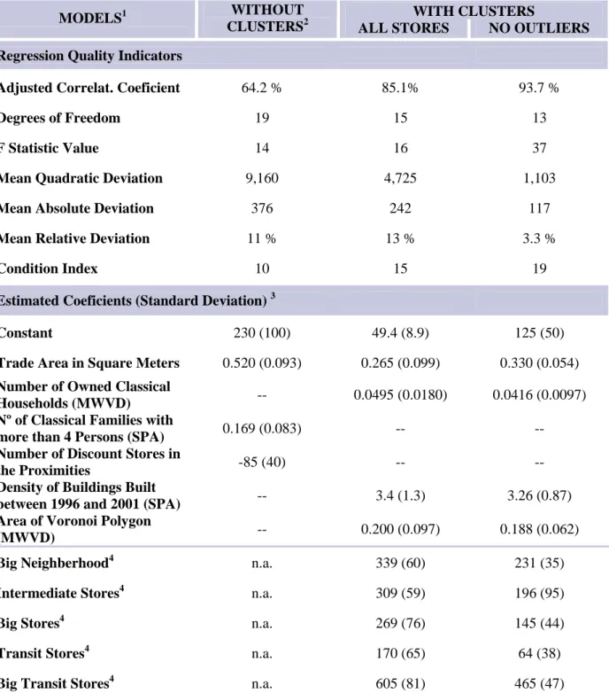
Of the results presented in Table 3 it is clear the need for segmenting the existing supermarkets. The best model without the inclusion of analogue groups is much inferior to the remaining two models that integrate that information, as all the quality indicators demonstrate. On the contrary, the models that include this information are very well fitted.

Table 3 – Linear regressions for the chain supermarkets with and without analogue groups (clusters). WITH CLUSTERS

MODELS1 WITHOUT

CLUSTERS2 ALL STORES NO OUTLIERS

Regression Quality Indicators

Adjusted Correlat. Coeficient 64.2 % 85.1% 93.7 %

Degrees of Freedom 19 15 13

F Statistic Value 14 16 37

Mean Quadratic Deviation 9,160 4,725 1,103

Mean Absolute Deviation 376 242 117

Mean Relative Deviation 11 % 13 % 3.3 %

Condition Index 10 15 19

Estimated Coeficients (Standard Deviation) 3

Constant 230 (100) 49.4 (8.9) 125 (50) Trade Area in Square Meters 0.520 (0.093) 0.265 (0.099) 0.330 (0.054) Number of Owned Classical

Households (MWVD) -- 0.0495 (0.0180) 0.0416 (0.0097) Nº of Classical Families with

more than 4 Persons (SPA) 0.169 (0.083) -- -- Number of Discount Stores in

the Proximities -85 (40) -- --

Density of Buildings Built

between 1996 and 2001 (SPA) -- 3.4 (1.3) 3.26 (0.87) Area of Voronoi Polygon

(MWVD) -- 0.200 (0.097) 0.188 (0.062) Big Neighberhood4 n.a. 339 (60) 231 (35) Intermediate Stores4 n.a. 309 (59) 196 (95) Big Stores4 n.a. 269 (76) 145 (44) Transit Stores4 n.a. 170 (65) 64 (38) Big Transit Stores4 n.a. 605 (81) 465 (47)

1

All the models are significative to 1% level by the F test and the estimated coeficients are significative to the 5% level by the t test.

2

The best model without any dummy variable. Several dependent variables and functional forms were tested. Two outleirs are excluded.

3

MWVD - Multiplicative Weighted Voronoi Diagrams, O2MWVD – Order 2 Multiplicative Weighted Voronoi diagrams, SPA - shortest path algorithms.

4

However, for the model that includes the outliers, the result is strongly influenced by these 2 supermarkets, namely in the mean relative deviation. In spite of that fact, comparing the results for the two best models is easy to conclude the good robustness of the obtained models since they use exactly the same predictor variables.

Although only a reduced number of predictors entered in the model, they are very well distributed by the classes suggested in the Figure 3. Actually, they include site and supermarket characteristic variables (offer) as the “trade area”, competition as the “area of Voronoi polygon”, the sales potential: in the “number of owned classical households” and dynamics using the “density of buildings built between 1996 and 2001”. Thus, in spite of the abundance of alternative predictor variables, the presence of key variables in the models is considered a minimum robustness condition (Themido et al., 1998).

Typically, the relative importance of predictors is assessed by simply comparing their standardized regression coefficients and (less often) by examining squared semipartial correlations. However, when variables are correlated, it is well recognized that regression coefficients cannot be used to unambiguously explain criterion variance that is shared by two or more predictors. While conducted within a stepwise regression framework, dominance analysis is an alternative analytic strategy that assesses the relative importance of more than one set of variables to prediction (Azen and Budescu, 2003, Budescu, 1993). This dominance analysis approach provides the most general context by taking into account all relevant subset models, where a relevant model is either any subset that can be formed from the predictors or that is theoretical possible and of interest.

Azen and Budescu (2003) define three levels of dominance. Complete dominance exists between two predictors if additional contribution of one predictor to each of the subset models is always grater than that of the other predictor. If the average additional contribution within each model size is greater for one predictor than the other, then that predictor is said to conditionally dominate the other. Finally if the overall average of the additional contribution is greater for one predictor than the other, that predictor is said to generally dominate the other. This general dominance measure coincides with the average squared

semipartial correlations across all combinations of predictors, advocated by Johnson (2000). In terms of interpretation, the general dominance represents the average difference in fit between all subset models (of equal size) that include a particular predictor and those that do not include it. The tree levels of dominance are related to each other in a hierarchical fashion: complete dominance implies conditional dominance, which in turn, implies general dominance. However, for more than three predictors the converse may not apply.

For each dependent variable the dominance analysis proceeds in two steps, following Budescu's (1993) guidelines. In step 1 several separate regression equations based on all possible ordering of sets of variables are computed. In step 2 the average multiple correlation coeficient for each set of variables, across all possible orderings of sets, are finally computed. Through this process an index is derived that represents the average usefulness of a set of predictors. From this index one can determine the percentage of variance accounted for by each variable set based on the total variance accounted for by the full model (Eby et al., 2003).

In Table 4 dominance analysis results are presented for the “best” forecasting regression

described in Table 3. Notice that these results are based in adjusted R2, which is recommended for comparisons between models with different number of predictors. It is easy to show that, adjusted R2 yields the same dominance pattern as any measure of model fit that is a monotone function of the model’s error sum of squares (Azen, 2000). The regressions correspond to a constrained dominance analysis as the dummy variables are always included in the models for theoretical reasons.

Examining the first row of Table 4 one can see that variable “Trade Area” (TA) has a greater contribution than any other variable, providing some initial evidence that TA is dominant to the other variables. Data from the other rows confirm this assertion. In fact, “Trade Area” (TA) completely dominates “Owned Households” (OH), which completely dominates “Buildings Built” (BB), which in turn dominates “Voronoi Area” (VA) considering de annual sales turnover explained variance. This analysis also indicates that VA contributes only significantly in models with 3 groups of variables (k = 3) contributing negatively in several of

the other models, indicating that the additional contribution doesn’t compensate for the redution of degrees of freedom. In spite of that the 3.7% explained variance increase in the

k

= 4

model may be relevant for forecasting accuracy.

Table 4 – Constrained Dominance Analysis for the “Best” Forecasting Regression.

ADDITIONAL CONTRIBUTIONS SUBSET MODELS* ADJUSTED

R2 TA OH BB VA k = 1 average 74.9% 6.7% 2.3% 0.2% -1.3%

(clusters) • Trade Area (TA) 81.5% 5.4% 1.4% 0.7% (clusters) • Owned Households (OH) 77.2% 9.8% 0.9% -1.4% (clusters) • Buildings Built (BB) 75.1% 7.9% 3.1% -0.8% (clusters) • Voronoi Area (VA) 73.6% 8.6% 2.3% 0.7%

k = 2 average 8.2% 3.3% 0.8% -0.7% (clusters) • TA • OH 87.0% 3.0% 0.9% (clusters) • TA • BB 83.0% 7.0% 2.9% (clusters) • TA • VA 82.2% 5.6% 3.7% (clusters) • OH • BB 78.2% 11.9% -0.9% (clusters) • OH • VA 75.8% 12.0% 1.5% (clusters) • BB • VA 74.3% 11.6% 3.0% k = 3 average 11.8% 5.2% 2.7% 1.0% (clusters) • TA • OH • BB 90.0% 3.7% (clusters) • TA • OH • VA 87.8% 5.9% (clusters) • TA • BB • VA 85.9% 7.8% (clusters) • OH • BB • VA 77.3% 16.4% k = 4 average 16.4% 7.8% 5.9% 3.7% (clusters) • TA • OH • BB • VA 93.7% overall average 10.8% 4.7% 2.4% 0.7% *

see

Table 3 for full variable names

.

For the regression without dummy variables representing the clusters, which is not constrained, it is also possible to determine complete dominance among the tree predictors in the order: “Trade Area” > “Number of Classical Families with more than 4 Persons” > “Number of Discount Stores” and for the regression without the identification of outliers the

results are very simillar to the ones presented in Table 4 with an inversion in the first two variables: “Owned Households” > “Trade Area” > “Buildings Built” > “Voronoi Area”. Note that the difference between the regressions with and without outliers is only two outliers which are included in the first and excluded in the last. In this way, we can conclude for the importance of outlier identification in regressions models and the high sensibility of adjusted multiple correlation coeficient and consequently dominance analysis to outliers. This is contraditory with bootstrap results presented in Azen and Budescu (2003) where the reproducibility values are very high. This contradiction is probably due to the instability of the regressions performed with very few data, as can be evaluated from the leave-one-out adjusted multiple correlation coeficient value presented.

5. Discussion and Conclusions

The retailers soon realised the importance of supermarket location, but understanding all the aspects of supermarket performance, site locations, and the consumer's behaviour, forces to collect enormous amounts of information of several types as geographical, demographic, socioeconomic and regarding competition dynamics (Hernández and Bennison, 2000, Themido et al., 1998, Salvaneschi, 1996). In this article spatial analysis data evaluation is carry out in a framework of a data analysis method for site selection and assessment, where three steps include several types of data and different data analysis procedures.

Variables obtained by four different methods are included in the study: two in store surveys to the customers of existent stores in two different years, a program of mystery shopping intended to record visible aspects of existing stores and new sites, geographical data that endorsed the calculation of competition variables, and census demographic data. The last two types of data employ spatial analysis to compute variables. Several delimitation models for influence areas are proposed namely based on algorithms of shortest path and in multiplicative weighted Voronoi diagrams (first and second order), combined with two methods of demographic variables aggregation. All six combinations are used in the calculation of demographic variables for explaining the 2002 annual sales turnover per area

ratio variance. From this analysis it is concluded that the model for the influence area delimitation is relevant in the calculation of spatial analysis data, driving to different models and with different sales explanatory power. On the contrary, one of the aggregation procedures, the decision rule aggregation, is superior to the other in the context of this study. Thus, this aggregation procedure is recommended and the multiplicative weighted Voronoi models are included in the GIS package and made available for future analyses. It should be noted that in the areas considered in the study the competition of nearby stores is particularly fierce.

Results from dominance analysis and other variable importance measures used for the other two steps confirm that variables from all categories in Figure 3 framework are identified. The importance of spatial analysis data is also very well established and considered fundamental only surpassed for the “trade area”, well known from the literature as a major factor (Themido

et al., 1998, Salvaneschi, 1996). For the delimitation model used, once more, all different

models are present and so the recommendation that all should be present in this kind of studies is supported.

We should also note the computation of several very similar variables as the “number of owned classical households (MWVD)”, which is very important in propositional classification rules and in the forecasting regression but with lower discriminant power than “density of owned classical households (O2MWVD)”, which is determined by a different influence area delimitation model and is a ratio between the number of classical households and the area of the Voronoi polygon. These results confirm the need to include several feature selection and extraction procedures in data analysis methodologies.

Dominance analysis starts with a clear definition of importance and identifies the measures that address the key question of comparing variable importance in predicting a target variable in the context of the variables included in the selected model (Azen and Budescu, 2003), and has the advantage of complying with all four theoretical characteristics identified by LeBreton et al. (2004). The same authors identify three conditions where importance measures may be particularly useful and yield different results as compared to standardized

regression coefficients when the following conditions are present: first, the predictors have a high level of multicollinearity; second, there are several predictors; and third, the predictors collectively explain a medium to large proportion of the variance in the dependent variable. For this particular data, dominance analysis is particularly adequate, and confirms the importance of the empirical variable classification suggested by Figure 3. The same results support the existence of structuring variables or key variables (see Themido et al., 1998) as the “trade area” which should always be present. Although the present results are not surprising, formal confirmations as the one presented in this work are seldom find in literature. In future works these results must be confirmed using other data sets from bigger supermarket chains.

6. References

Azen, R. (2000). Inference for predictor comparasions: Dominance analysis and the distribution of R2 differences. Dissertation Abstracts International, B 61/10, pp. 5616.

Azen, R. and D. Budescu (2003). The dominance analysis approach for comparing predictors in multiple regression. Psycohological Methods, 8 (2), pp. 129-148.

Berg, M., M. van Kreveld, M. Overmars and O. Schwarzkopf (2000). Computational

Geometry: Algorithms and applications. Berlin: Springer-Verlag.

Biggs, D.B.V. and E. Suen (1991). A method of choosing multiway partitions for classification and decision trees. Journal of Applied Statistics, 18, pp. 49-62.

Birkin, M., G. Clarke and M. Clarke (2002). Retail Geography and Intelligent Network

Planning. Chichester, UK: John Wiley & Sons.

Boots, B. (2002). Using local statistics for boundary characterization. In: B. Boots, A. Okabe and R. Thomas (eds.), Modelling Geographical Systems: Statistical and computational

applications. Dordrecht, Netherlands: Kluwer Academic Publishers, pp. 33-44.

Boots, B. and R. South (1997). Modeling retail trade areas using higher-order, multiplicatively weighted Voronoi diagrams. Journal of Retailing, 73 (3), pp. 519-536.

Breiman, L., J. H. Friedman, R. A. Olshen and C. J. Stone (1984). Classification and

Regression Trees. California, USA: Wadsworth International.

Budescu, D.V. (1993). Dominance analysis: A new approach to the problem of relative importance of predictors in multiple regression. Psychological Bulletin, 114 (3), pp. 542-551. Cardoso, M. G. M. S. and L. Moutinho (2003). A logical type discriminant model for profiling a segment structure. Journal of Targeting, Measurement and Analysis for Marketing 12 (1), pp. 27-41.

Church, R. L. (2002). Geographical information systems and location science. Computers

Cowen, D. J., J. R. Jensen, W. L. Shirley, Y. Zhou and K. Remington (2000). Commercial real estate GIS site evaluation models: Interfaces to ArcView GIS. In Proceedings of the 20º

Annual ESRI International User Conference. ESRI online Library, pp. 140-145.

Crask, M. R. and W. D. Perreault (1977). Validation of discriminant analysis in marketing research. Journal of Marketing Research, 11 (February), pp. 60-64.

Davies, R. L. and D. S. Rogers (1984). Store Location and Store Assessment Research. Chichester, UK: John Wiley & Sons.

Dawson, J. (2000). Retailing at century end: Some challenges for management and research. The International Review of Retail, Distribution and Consumer Research, 10 (1), pp. 119-148.

Dirichlet, P. G. L. (1850). Über die reduction der positiven quadratischen formen mit drei umbestimmten ganzen Zahlen. Journal für die Reine und Angewandte Mathematik, 40, pp. 209-227.

Eby, L. T., M. Butts and A. Lockwood (2003). Predictors of success in the era of the boundaryless career. Journal of Organizational Behavior, 24 (6), pp. 689-708.

Eurostat (2001). Distributive trades in Europe. Luxembourg: Office for Official Publications of the European Communities.

Eurostat (2003). European Business Facts and Figures, Part 5: Trade and tourism, data

1991-2001. Luxembourg: Office for Official Publications of the European Communities.

Gentle, J. E. (2002). Elements of Computational Statistics. New York, USA: Springer-Verlag. Gilbert, D. (2002). Retail Marketing Management. Upper Saddle River, USA: Prentice Hall. Hernández, T. and D. Bennison (2000). The art and science of retail location decisions.

International Journal of Retail & Distribution Management, 28 (8), pp. 357-367.

Johnson, J. W. (2000). A heuristic method for estimating the relative weight of predictor variables in multiple regression. Multivariate Behavioral Research, 35, pp. 1-19.

Jones, M. A., D. L. Mothersbaugh and S. E. Beatty (2003). The effects of locational convenience on customer repurchase intentions across service types. The Journal of

Services Marketing, 17 (7), pp. 701-712.

Kass, G. (1980). An exploratory technique for investigating large quantities of categorical data. Applied Statistics, 29 (2), pp. 119-127.

Lattin, J., J. D. Carroll and P. E. Green (2003). Analysing Multivariate Data. Pacific Grove, USA: Duxbury.

LeBreton, J. M., R. E. Ployhart and R. T. Ladd (2004). A Monte Carlo comparison of relative importance methodologies. Organizational Research Methods, 7 (3), pp. 258-282.

Lilien, G. L., P. Kotler and K. S. Moorthy (1992). Marketing Models. New Jersey, USA: Prentice Hall International.

Loh, W. Y. and Y.-S. Shih (1997). Split selection methods for classification trees. Statistica

Sinica, 7, pp. 815-840.

McGoldrick, P. (2000). Retail Marketing. London, UK: McGraw-Hill Europe.

McMullin, S.K. (2000). Where are your customers: Raster based modeling for customer prospecting. In Proceedings of the Annual ESRI International User Conference. ESRI online Library, pp. 795-823.

Mendes, A. B. and M. G. M. S. Cardoso (2005). Clustering Supermarkets: The role of experts. Journal of Retailing and Consumer Services (in press).

Mendes, A. B. and I. H. Themido (2004). Multi outlet retail site location assessment: A state of the art. International Transactions in Operations Research, 11 (1), pp. 1-18.

Moutinho, L., M. Goode and F. Davies (1998). Quantitative Analysis in Marketing

Management. Chichester, UK: John Wiley & Sons.

Okabe, A., B. Boots, K. Sugihara and S. N. Chiu (2000). Spatial Tessellations: Concepts and

applications of Voronoi diagrams. Chichester, UK: John Wiley & Sons.

Okabe, A. and A. Suzuki (1997). Locational optimization problems solved through Voronoi diagrams. European Journal of Operational Research, 98 (3), 445-456.

Pioch, E. and J. Byrom (2004). Small independent retail firms and locational decision-making: Outdoor leisure retailing by the crags. Journal of Small Business and Enterprise

Development, 11 (2), pp. 222-232.

Quinlan, J. R. (1993). C4.5: Programs for machine learning. San Mateo, USA: Morgan Kaufmann Publishers.

Salvaneschi, L. (1996). Location, Location, Location: How to select the best site for your

business. Grants Pass, USA: Psi Research - Oasis Press.

Seth, A. and G. Randall (1999). The Grocers: The rise and rise of the supermarket chains. London, UK: Kogan Page.

Shieh, Y.-N. (1985). K.H. Rau and the economic law of market areas. Journal of Regional

Science, 25 (2), pp. 191-199.

Themido, I., A. Quintino and J. Leitão (1998). Modelling the retail sales of gasoline in a Portuguese metropolitan area. International Transactions in Operations Research, 5 (2), pp. 89-102.

Voronoï, G. (1908). Nouvelles applications des paratrés continus à la théorie des formes quadratiques. Deuxième memoie, recherche sur les parallelloèdres primitif. Journal für die

Reine und Angewandte Mathematik, 134, pp. 198-287.

Wedel, M. and W. A. Kamakura (2000). Market Segmentation: Conceptual and