Predicting the probabilities of default for the
banking sector in the United States
Lukas Weisel
Dissertation written under the supervision of Nuno Silva
Dissertation submitted in partial fulfilment of requirements for the MSc
in Economics, at the Universidade Católica Portuguesa, 08.01.2020
Abstract
Title: Predicting the probabilities of default for the banking sector in the United States Author: Lukas Weisel
Key words: Structural credit risk models, Banking, Probability of Default
This dissertation implements a structural credit risk model to predict the probabilities of default for the eight largest retail banks in the United States. Similar to Goldstein, Ju, and Leland (2001), the model implemented in this dissertation relates the project/asset value with the firm capacity to generate earnings. Most papers in the literature consider that firms have fixed financial costs and that shareholders decide whenever to liquidate the firm based on the distance between some underlying earnings measure and these fixed costs. This assumption is not reasonable in the case of banks. As an alternative to incorporate shareholders strategic default decision, non-financial fixed costs are considered. These non-financial fixed costs are defined as the non-interest expenses and proxy the operational leverage of the bank. The analysed sample period contains 19 consecutive years, covering the dotcom crisis, the financial crisis and several minor crises in between. The model was calibrated by applying the iterative approach proposed by Vassalou and Xing (2004). The average computed probability of default for the whole sector ranged between 0.06% in 2006 and 5.80% during the financial crisis. These results were compared with the probabilities of default and the distances-to-default implied by Moody’s and Standard & Poor’s credit ratings for the period between 2006 and 2018. Though the probabilities of default show a low not significant correlation, the distances-to-default have a correlation of 53.27%, which was found to be significant at the usual significance levels.
Resumo
Título: Previsão das probabilidades de incumprimento para o sector bancário nos Estados Unidos
Autor: Lukas Weisel
Palavras-chave: Modelos de risco de crédito estrutural, Banca, Probabilidade de inadimplência
Esta tese implementa um modelo estruturado de risco de crédito para prever as probabilidades de falência dos oito maiores bancos comerciais nos Estados Unidos. Com base no trabalho de Goldstein, Ju and Leland (2001), o modelo implementado compara o valor do projeto/ativo com a capacidade da empresa de gerar receitas. A maioria da literatura considera que as empresas têm custos financeiros fixos e que os acionistas decidem liquidar a empresa sempre que se verificar uma determinada diferença entre as receitas e estes custos fixos. Esta premissa, no entanto, não é razoável no caso dos bancos. Como alternativa para a decisão estratégica dos acionistas de liquidar o banco, são também considerados custos fixos não-financeiros. Estes custos são definidos como despesas sem juros, representando um valor aproximado da alavancagem operacional do banco. O período analisado é composto por 19 anos consecutivos, cobrindo principalmente a crise da bolha da internet e a crise financeira de 2007/08. O modelo foi construído aplicando a abordagem sugerida por Vassalou e Xing (2004). A probabilidade média de falir calculada varia entre 0.06% em 2006 e 5.80% durante a crise financeira. Estes resultados foram comparados com as probabilidades de falência e distâncias para a falência calculadas pela Moody’s e Standard & Poor’s para o período entre 2006 e 2018. Apesar das probabilidades de falência demostrarem uma correlação baixa e não significante, as distâncias para a falência têm uma correlação de 53.27%, sendo significante para os usuais valores de significância.
Acknowledgements
First of all, I would like my supervisor Nuno Silva for his constant effort with any problems and the excellence of his teaching ability. Without any hesitation he provided a high-level support that enabled me to develop my knowledge in this area. Further I would like to thank the Católica Lisbon School of Business and Economics for the practical relevance of the materials taught throughout the whole programme.
Especially, I want to thank my family for their support over all these years to contribute perceiving this master. Without your support this wouldn’t have been possible.
Finally, I would like to thank all the friends that I was able to get to know over the last one-and-a-half years. You were always supportive, made me feel like being in good company, and enhanced this whole experience.
Table of Contents ABSTRACT ... 2 RESUMO ... 3 ACKNOWLEDGEMENTS ... 4 INDEX OF TABLES ... 7 INDEX OF FIGURES ... 7 INDEX OF APPENDIX ... 8 1. INTRODUCTION ... 9 2. LITERATURE REVIEW ... 12 2.1STRUCTURAL MODELS ... 12
2.2STRUCTURAL MODELS APPLICATIONS TO THE BANKING SECTOR ... 14
3. MODEL ... 18
3.1EBIT-BASED MODEL (GOLDSTEIN,JU,LELAND,2001) ... 18
3.2ADAPTING GJL MODEL TO THE BANKING SECTOR ... 22
4. DATA INPUTS AND MODEL CALIBRATION ... 23
4.1CALIBRATION OF THE GJL(2001)-MODEL ... 23
4.1.1 ITERATIVE APPROACH –ASSET VALUE AND ASSERT RETURN VOLATILITY ... 23
4.1.2 COMPUTATION OF THE MARKET PRICE OF RISK ... 24
4.2DATA INPUTS ... 25
4.2.1IMMEDIATE VARIABLES... 25
4.2.2ITERATIVELY OBTAINED VARIABLES... 34
5. RESULTS ... 36
5.1CREDIT RISK INDICATORS ... 36
5.1.1DEFAULT BARRIER-TO-ASSET RATIO... 36
5.1.2DRIFT OF THE PROCESS 𝜇𝑝 ... 37
5.1.3DISTANCE-TO-DEFAULT (5-YEAR)... 38
5.1.4PROBABILITIES OF DEFAULT (5-YEARS) ... 40
5.2COMPARISON TO RATING AGENCIES ... 43
5.2.1IMPLIED PROBABILITY OF DEFAULT FROM RATING AGENCIES ... 43
6. CONCLUSION ... 48 REFERENCES ... 49 APPENDIX ... 51
Index of Tables
TABLE 1 – BANKS SELECTED ... 23
TABLE 2 – INPUTS AND THEIR SOURCES ... 25
TABLE 3 – SHAPIRO-WILK TEST FOR NORMALITY ... 26
TABLE 4 – SKEWNESS OF COMPANIES’ STATE VARIABLE ... 26
TABLE 5 – KURTOSIS OF THE COMPANIES’ STATE VARIABLE ... 27
TABLE 6 – MEAN BETA COEFFICIENT 𝛽 ... 30
TABLE 7 – ANNUALIZED EQUITY VOLATILITY Σ_E ... 31
TABLE 8 – AVERAGE EXPECTED RATE OF RETURN ON EQUITY 𝜇𝑒 ... 32
TABLE 9 – MEAN MARKET PRICE OF RISK 𝜃 ... 32
TABLE 10 – PROJECTS VOLATILITY Σ_V ... 34
TABLE 11 – PAYOUT RATIO FOR EACH COMPANY ... 35
Index of Figures
FIGURE 1 – QUARTERLY EQUITY VALUES (IN MILLIONS $) ... 27FIGURE 2 – QUARTERLY EQUITY VALUES (IN MILLIONS $) ... 28
FIGURE 3 – HISTORICAL FREE CASHFLOW TO EQUITY COMPARISON ... 29
FIGURE 4 – HISTORICAL BETA COEFFICIENTS 𝛽 ... 29
FIGURE 5 – INTEREST RATE ... 31
FIGURE 6 – MARKET PRICE OF RISK BOXPLOT ... 33
FIGURE 7 – PANEL A (MARKET PRICE OF RISK) ... 33
FIGURE 8 – PANEL B (MARKET PRICE OF RISK) ... 34
FIGURE 9 – DEFAULT BARRIER-TO-ASSET RATIO ... 37
FIGURE 10 – DEFAULT BARRIER-TO-ASSET RATIO ... 37
FIGURE 11 – DRIFT OF THE PROCESS 𝜇𝑝 ... 38
FIGURE 12 – DRIFT OF THE PROCESS 𝜇𝑝 ... 38
FIGURE 13 – QUARTERLY DD OF COMPANIES ... 39
FIGURE 14 – QUARTERLY DD OF COMPANIES ... 39
FIGURE 15 – QUARTERLY PROBABILITIES OF DEFAULT ... 40
FIGURE 16 – QUARTERLY PROBABILITIES OF DEFAULT ... 41
FIGURE 17 – CREDIT RATING IMPLIED PROBABILITIES OF DEFAULT AND MODEL COMPARISON ... 43
FIGURE 18 – SCATTER PLOT OF MODEL AND IMPLIED RATING PROBABILITIES OF DEFAULT ... 44
FIGURE 20 – CORRELATION OF RATING AGENCIES AND MODEL DD'S ... 46
FIGURE 21 – MERTON OUTPUT AND DD'S COMPARISON ... 47
Index of Appendix
APPENDIX 1 – NON-INTEREST EXPENSE (IN $ MILLION) ... 51APPENDIX 2 – EARNINGS BEFORE TAXES (IN MILLIONS $) ... 51
APPENDIX 3 – STATE VARIABLE (IN MILLIONS $) ... 52
APPENDIX 4 – YEARLY 5-YEAR PROBABILITIES OF DEFAULT (PD) ... 53
APPENDIX 5 – BARRIER-TO-ASSET RATIO ... 53
APPENDIX 6 – DISTANCE-TO-DEFAULT YEARLY VALUES (DD) ... 54
APPENDIX 7 – YEARLY DRIFT OF THE PROJECT 𝜇𝑝 ... 54
APPENDIX 8 – IMPLIED PROBABILITIES OF DEFAULT (S&P) ... 55
APPENDIX 9 – IMPLIED PROBABILITIES OF DEFAULT (MOODY'S) ... 55
APPENDIX 10 - INVERSE NORMAL FUNCTION ON MODEL PD'S (YEARLY RESULTS) ... 56
1. Introduction
Banks mainly generate earnings from three different sources. First, through the so-called interest rate margin. The main task of a retail bank is to collect deposits, for which they pay interest, and to grant credit to customers, to which they charge interest. This difference is expectedly positive. Second, banks charge commissions on their payment services or similar. Third, banks earn interest and dividends from investing in government or rated assets. The business model just described leaves banks exposed to a variety of different sources of risk. Three in particular, notably, credit, liquidity risk and market risk. Credit risk is defined as the risk that emerges from customers that are unable to repay their loan or contractual obligations towards the bank. Once this risk materialises it includes lost principal and interest, while increasing collection costs for the bank. Especially during the subprime crisis many banks suffered from significant losses through loans towards high-risk borrowers. These were caused by subprime mortgage borrowers. This can be measured by banks stating it as a “loss given default”, which monitors the amount that got lost due to the default. The liquidity risk emerges from maturity transformation, which appears from the different maturity characteristics of deposits and loans. Short-term deposits are used to create long-term loans, which limit the banks financial resources in the case that depositors want to take their money out. Market risk emerges from the investing of some of the retail banks liquidity in bonds and other tradable securities, like government bonds or similar low-risk assets. Banks are measuring their market risk by using the value-at-risk (VaR) approach. It can be defined as the maximal value that a portfolio can suffer from and is known as one of the predominant risk management approaches used by banks (Berkowitz and O’Brien, 2002). Even though these are generally perceived as low-risk assets they increase their exposure to the market and create market risk. Operating risk can arise from employee errors, fraud or events that disrupt the production process. These can cause losses for the company. The economy is in demand of capital, which can cause banks to develop risk-taking incentives, which can be a problem in combination with the naturally low level of equity hold. The amount of capital held by a bank is measuring the potential amount a bank can absorb. Due to an increase in the return on equity that banks can achieve by using debt instead, the banks are holding only a low amount of capital. Debt is cheaper than equity, because the level of equity in a company can only be increased by retaining profits, decreasing dividend payments or buying shares back. Banks prefer not to use these options as they are not in line with shareholders wants or highly costly. Consequently, regulators aim to increase this low
level of capital to prevent bailouts paid by taxpayers as the capital is used to absorb losses when risks materialise.
Given that banks have a critical role in the economy and the risks that they face, they are regulated institutions. These regulations are intended to work as a framework to create a safer environment for companies and prevent financial crises. These regulations contain capital requirements that must be fulfilled by banks to be allowed to operate. In the last years, buffer requirements for cyclical risk were also added to the regulatory framework. This risk emerges from the cyclical peaks and downturns, which can have a significant effect on the business cycles of companies. Nevertheless, it is safe to say that these regulations are supposed to work as a financial cushion towards losses and prevent banks from overly taking risk into their books, but they don’t guarantee that a bank cannot go bankrupt.
Several methodologies were proposed to measure the probability of banks going bankrupt. One of those methodologies are structural credit risk models. Structural credit risk models can be applied to overcome some of the previously defined shortcomings of traditional risk management metrics and models to predict the probabilities of default of financial institutions. Structural models use market data, which allow them to create forward-looking results. Consequently, this type of data enables the model to predict with a higher rate of precision and a more market realistic way.
Credit risks’ close link towards default caught up the interest of many researchers and academics. For this reason, we are applying a structural model to analyse their exposure towards risk and analyse the likelihoods of default during times of crisis. In comparison to the previously mentioned approaches, structural models are very complex and difficult to successfully apply to financial institutions from an empirical perspective. Nevertheless, this dissertation aims towards the implementation of a structural model to predict the probabilities of default for the financial sector in the United States. In order to achieve this, a data set that contains 19 years of data from the eight largest retail banks in the United States is analysed. The model implemented in this dissertation is a modified version of the static Goldstein, Ju, Leland (2001) model, which is an EBIT-based structural model. This model finds application in the prediction process of the probabilities of default of these companies and therefore can retrieve information about their performance during the dotcom-crisis, the financial crisis of 2008, and an increase around 2014 – 2015 due to market changes. Throughout this time period, it was possible to retrieve information about the performance of the eight largest retail banks in the United States, which are an employer for many people and financial providers for a whole nation, that almost went bankrupt or that had to be bailed out. Finally, the probabilities retrieved from the GJL
(2001)-model were compared with the implied probabilities of default from the credit ratings of professional agencies. Further, the probabilities of default were used to compute the DD’s and compare these with the rating implied ones by applying an InverseNormal function. The structure of the dissertation is following the order of: Chapter 2 – Literature Review, Chapter 3 –Model, Chapter 4 – Data Inputs and Model calibration, Chapter 5 – Results, and finally in Chapter 6 – Conclusion.
2. Literature Review
2.1 Structural modelsThe application of structural credit risk models can be traced back to the pioneering papers of Black and Scholes (1973) and Merton (1974). In these papers corporate securities are seen as contingent claims on a firm’s underlying assets. In the beginning, the pioneering paper of Black and Scholes (1973) first proposed an explicit formula to price call options on common stocks. Following joint work with Merton they also stated that in the hypothetical case of a company that issued a single pure discount bond and has a predetermined liquidation date, equity can be seen as a call option on the firm assets with strike equal to nominal liabilities. Thus, the Black-Scholes formulas could be used to price stocks. Therefore, this framework could be used to measure the value of equity. While the debt can be valued by applying put-call parity. This makes debt a covered call or something equivalent to a risk-free loan implied by a short put option. The put premium in this case can be understood as a compensation for the default risk. From this on it is possible to compute the probabilities of default with this framework. These are defined as the probability with which the company is unable to meet their outstanding financial obligations (Merton, 1974). The Black-Scholes formula used the market value of assets, the asset volatility, the risk-free rate, time-to-maturity, and the face value of debt as the strike price of the option (Black & Scholes 1973). This approach to measure credit risk became known as the Merton model. The usage of market data enables the prediction of forward-looking results and therefore are one of the main advantages of structural credit risk models. Black and Cox (1976) improved on Merton’s model by disbanding the assumption that companies can only default once outstanding debt matures. In their model the company defaults when the asset value passes a certain barrier the first time. They justify that default can occur at any point in time with the company not being able to meet its collateral agreements. The possibility of early default makes the model more realistic. They were the first ones to propose the “first passage time model”. Everything else equal, the introduction of the possibility of early default leads to an increase in the chances of the firm defaulting. However, in contrast to Merton model where the asset value of a company can sink to any level before the debt is maturing, in Black-Cox debt holders’ losses are capped by the recovered value at the barrier (Black & Cox, 1976).
A more complex approach was proposed by Geske (1977). In this paper, every time a payment is due shareholders have to decide whether or not do default. Shareholders exercise the option to stay when the asset values are at a significantly high level, which makes it possible to raise
new equity and continue with the payments to creditors. In contrast, they abandon the firm when the asset value is reaching a predefined low level where it is not possible to raise enough equity to meet the financial obligations to the creditors. The latter leads to the takeover of the company's assets by the creditors (Imerman, 2011). This approach was first proposed by Geske and further developed by Geske and Johnson (1984). This mechanism can further be compared to the one of compound options. These are defined as an option, which underlying asset is also an option. Therefore, these obtains can widely be applied through the possible combinations of call and put options. The advantage of this is that the bank got an exposure towards the underlying option now, but by hedging the exposure due to long-term costs of paying for the option now. Companies can therefore use these options while planning on costly projects and secure financial sources before going into the project. If they are unable to realize the project, they just lose their exposure towards the option, but without initiating costs of financing the unrealized project. Hence, financial institutions gain a sort of insurance policy from using compound options (Geske, 1979).
As this dissertation is about the computation of probabilities of default as important indicators in credit risk models it is essential to mention the paper about public firm expected default frequency (EDF), authored by Sun, Munves, and Hamilton (2012). Their paper follows the analytical calculation approach of default frequencies and their model belongs to the class of structural credit risk models. Their approach contains the distance-to-default (DD) which is of special interest for this dissertation. This approach first got proposed by Moody’s KMV expected default frequency risk calculation model (Crosbie and Bohn, 2003). It represents a count of standard deviations that the asset value is away from financial distress, while assuming that there is a normal distribution. Hence, the distance-to-default can be seen as a market-based approach of corporate default risk, due to his inputs of the market value of the asset, the default point and the asset volatility. The measure captures macro-economic and firm-specific events in a closed-form solution, which can be seen as an advantage towards the classic Merton model (Crosbie and Bohn, 2003). They define the numerator as the difference between the logarithm of the asset value and the logarithm of the default point, which captures the firms' leverage. Meanwhile, the denominator discounts the leverage of the firm by asset volatility and therefore captures the denominator. Further, it can capture the overall risk level through the asset volatility. This formula can be used as a base to enhance the amount of credit risk parameters in a dissertation, which is using market information. The usage of market information allows forward-looking solutions towards default risk.
Brockman and Turtle (2003) proposed in their paper another approach using a barrier. In their paper, they proposed to use the down-and-out call (DOC) valuation model of Merton (1974). The DOC framework works through exercising the call option once the barrier is hit and therefore terminates the company transferring the asset values from asset ownership to creditors (Brockman and Turtle, 2003). They find that this implication of a barrier leads to dominating results compared to the accounting-based approach of Altman Z-scores in almost all of their 7,787 firm-years tested.
In addition to the previously mentioned papers, there is a vast literature determined towards structural models that cover important corporate finance questions. These papers should be mentioned as well, due to their assumptions and findings. These can further be used to enhance structural models for the computation of default probabilities.
In the paper of Leland (1994), tax rates and bankruptcy costs are introduced, which allows the author to analyse the optimal capital question. In this model they assume that the shareholders set an endogenous threshold barrier at the lowest asset value where equity is still positive. The model assumes one class of debt with a fixed coupon and an infinite maturity. Once the asset value of the bank is reaching the barrier the shareholders make the strategical decision to default the company.
Goldstein, Ju, and Leland proposed a model that is using a cash flow-based approach to predict the optimal capital structure in a dynamic setting (i.e. they consider the possibility of issuing further debt in the future). They state that most models are limited by a static capital structure, while assuming a dynamic capital structure has significant effects on the amount of initial debt issued and the risk linked to these bond issuing companies. They assume that companies, in reality, adjust their debt levels with changing firm values and therefore tackle these previous assumptions (Goldstein, Ju, Leland, 2001).
The Leland- and the GJL-model are two examples of especially interesting corporate finance papers that can provide important insights to the measure of probabilities of default.
2.2 Structural models applications to the banking sector Some papers using structural models focus on the banking sector.
Episcopos (2007) adapts the model proposed by Brockman and Turtle (2003) to the banking sector. This paper finds that their barrier option model is useful for bank regulators. Stockholders are left behind with a down-and-out call option, which leads to a decrease in their incentive to increase asset risk. As an increase in the regulatory barrier leads to a wealth transfer
from shareholders to in their case the federal deposit insurance corporation. This can be understood as a management tool for a deposit insurance premium schedule (Episcopos, 2007). The model assumes closure barriers to become trivial, while the down-and-in option works as a prompt corrective action (PCA). Thus, the barriers can be used as policy tools for banks and other financial institutions to meet capital requirements and restrictions from regulators (Episcopos, 2007).
Further, Flannery (2005) assumed in his work that asset values follow different stochastic processes. This could be taken into account for inputs in structural models to compute more realistic results. Assets following this assumption could increase the analysing power of banks capital structure works in times of financial crisis and how the valuation of contingent capital is affected by declines in the asset value, as more extreme events could be captured. This assumption could be applied to predict default probabilities through a structural model and retrieve information about the difference in their performance.
Following the previous assumption of asset values that follow different stochastic processes, Pennacchi (2010) stated the assumption that banks asset values follow a jump-diffusion process, while the bank issues short-term deposits, shareholder’s equity, and fixed- or floating-coupon contingent capital bonds (Pennacchi, 2010). The papers goal is to find evidence about the pricing mechanism of contingent capital in times of financial distress and how credit spreads are evolving at this time in the case of issuing banks. Further, they explore the risk-taking incentives of banks that issue several forms of contingent claims compared to banks that offer non-convertible subordinated debt. They find that banks that issue contingent capital are more likely to face moral hazard incentives to increase their asset's jump risk. In addition, they find that contingent capital is a feasible and cost-saving opportunity to mitigate financial distress when it is targeted to transform at an early stage (Pennacchi, 2010).
First of all, the implication of a jump-diffusion process, which permits sudden declines in asset values, led to contingent claims, that normally would have been risk-free or contain zero credit spreads, becoming positive. This provides more realistic results in times of crisis. They find that credit spreads of contingent claims tend to have an inverse relationship with the bank's capital, which can be explained through the closer range to conversion. Regarding the risk-taking incentive, they couldn't find evidence that a bank is issuing contingent capital to transfer value from contingent claims investors to banks shareholders because this incentive is given when issuing comparable subordinated debt as well (Penachhi, 2010). Even though earnings that follow a jump-diffusion process can monitor sudden declines in a better way, the
geometric-Brownian motion process, that is used by a lot of models, is also able to display declines realistically.
Due to the increasing connection of the global economy and the key role financial institutions take in this, it is important to predict future probabilities of default with a high level of precision. Even non-systemic crises can cause high costs for the public through bailouts of companies, that are defined to be systematic. Consequently, structural models can also be used to predict the likelihood with which banks are in need of a bail-out and the costs linked to these. Correia, Dubiel-Teleszynsky, and Población (2017) applied a Leland (1994)-style model, as it allows to model a more realistic approach and has the advantage of cash flows as an observable variable and the opportunity to model changes in the tax rate. Therefore, their model can indicate times with higher likelihoods of default and the costs that would occur out of it. These findings could help governments to work out regulations to increase their performance in a crisis. They find that the main costs of banking bailouts are caused by equity injections, deposit insurances and loan guarantees (Correia, Dubiel-Teleszynsky & Población, 2017).
Structural models can further be used towards the pricing of hybrid securities. These represent an important way for banks to raise capital in times of liquidity and/or market risk. The so-called reverse convertible debentures (RCD) could be analysed in future literature towards its effect to lower probabilities of default. This financial instrument would automatically convert into common equity once a market capital ratio of a bank reached a predetermined level. The current stock market price is used when the RCD converts, which hands over the full cost to shareholders, as a price of their risk-taking decision (Flannery, 2005). Structural models could therefore also be used to pursue the likelihood of a government bailout and therefore be in the interest of national supervisors. Further research could implement this kind of financial instrument towards a structural model and predict their efficiency to reduce the probabilities of default. In the case that good results, the government could create regulations towards banks to require them to hold a specific amount of these instruments like a capital requirement does for equity.
Additionally to the previous findings for hybrid securities, they seem to be a lower-cost alternative towards equity allowing for tax advantages (Barucci & Del Viva, 2013). Barucci and Del Viva apply an option pricing formula for contingent convertible-bonds (Coco-bonds). These provide financial services for banks, deleverage bank's balance sheets in times of high financial risk and reduce the expected bankruptcy costs while increasing the stability of the financial sector. Therefore, this financial instrument can reduce the likelihood of bankruptcy significantly in times of financial crisis. Overall they state that this instrument provides a lower
bankruptcy barrier and lower bankruptcy costs. Even though the instrument can do this for a company it comes at the cost of a higher yield spread of callable bonds, which is equivalent to an increase in the insurance premium (Barucci & Del Viva, 2013). Hence, several more instruments could be tested by structural models to predict if they can actively lower the probabilities of default for retail banks.
3. Model
The model used in this dissertation is largely based on the static version of Goldstein, Ju and Leland (2001) EBIT-based structural model. In this chapter, this model is explained in-depth and followed by a part about the calibrations of the model that were applied.
3.1 EBIT-based Model (Goldstein, Ju, Leland, 2001)
Goldstein, Ju and Leland (2001) assume that a company holds a project that generates a payout
flow. The dynamics of this payout flow under measure P are given by1
Equation 1
𝑑𝛿
𝛿 = 𝜇𝑃𝑑𝑡 + 𝜎𝑑𝑧,
where 𝜇𝑝 and 𝜎 are constants. Here, 𝜇𝑝, describes the drift of the project, while 𝜎 describes the
volatility of the project returns. This equation is stated under the physical measure P. The physical measure P is true probability measure, which needs to be used to predict the probabilities of default later on. By discounting all expected future earnings flows at a certain constant discount rate, the project value can be obtained. Precisely, the value of the claim to the earnings flow is Equation 2 𝑉(𝑡) = 𝐸𝑡𝑄(∫ 𝑑𝑠𝛿𝑠𝑒−𝑟𝑠 ∞ 𝑡 ) = 𝛿𝑡 𝑟−𝜇,
where 𝜇 = (𝜇𝑃− 𝜃𝜎) is usually called the risk-neutral drift and 𝑟 describes the risk-free rate.
Both are assumed to be constant. 𝜃 is the market price of risk. The market price of risk is the compensation that investors require to invest in a certain project by a unit of risk. The risk premium is described by 𝜃𝜎. By applying Ito’s lemma to the previously defined project value function, one can obtain the project value dynamics. This can be written under measure P
(equation 3a) or under measure Q (equation 3b):2
Equation 3a
𝑑𝑉
𝑉 = 𝜇𝑃𝑑𝑡 + 𝜎𝑑𝑧
𝑃
1 A probability measure is a function that gives probabilities to states of the world.
2 Measure Q is an alternative probability measure. Similar to measure P, measure Q gives probabilities to states
Equation 3b
𝑑𝑉
𝑉 = 𝜇𝑑𝑡 + 𝜎𝑑𝑧
𝑄.
It is clear from equation 1 and 3a that V and 𝛿 share the same dynamics under measure P (i.e.
both follow a geometric Brownian motion with drift 𝜇𝑃 and volatility𝜎). The same is true under
measure Q.
Now, define the project payout ratio k as the ratio of the payout flow and the project value. In this case we have that:
Equation 4
𝑘 =𝛿𝑡
𝑉 = 𝑟 − 𝜇.
By rearranging equation 4, we can obtain the following:
Equation 5
𝜇 = 𝑟 − 𝑘.
Substituting 𝜇 from equation 3b and rewriting the process, one obtains
Equation 6
𝑑𝑉
𝑉 = (𝑟 − 𝑘)𝑑𝑡 + 𝜎𝑡𝑊𝑡
𝑄.
The value of any contingent claim on this asset can be found by solving the below partial differential equation (PDE):
Equation 7 (𝑟 − 𝑘)𝑉𝐹𝑣+ 𝜎2 2 𝑉 2𝐹 𝑉𝑉+ 𝐹𝑡+ 𝑃 = 𝑟𝑓,
where P in this case is defined as the payout flow specific to the contract we want to price. In the case of time independent securities, this PDE reduces to a second-order ordinary differential equation (ODE): Equation 8 0 = (𝑟 − 𝑘)𝑉𝐹𝑣 +𝜎2 2 𝑉 2𝐹 𝑉𝑉+ 𝐹𝑡+ 𝑃 − 𝑟𝑓,
We are interested in finding a pricing function (called F function in this case) that fulfils the condition given by equation 8 and the characteristics of the contract we want to price. The solution to equation 8 is generally found as the sum of the general solution to the homogenous equation, where the payout associated with the claim is equal to zero (i.e. P=0), and adding a particular solution. This particular solution depends on the contract we want to price. In our model, we will assume that the firm defaults whenever V falls to a certain level, hereafter
The general solution to the above second-order ordinary differential equation is given by Equation 9 𝐹𝐺𝑆 = 𝐴1𝑉−𝑦+ 𝐴2𝑉−𝑥, where Equation 10 𝑥 = 1 𝜎2[(𝜇 − 𝜎2 2) + √(𝜇 − 𝜎2 2) 2 + 2𝑟𝜎2] and Equation 11 𝑦 = 1 𝜎2[(𝜇 − 𝜎2 2) − √(𝜇 − 𝜎2 2) 2 + 2𝑟𝜎2].
In the case of a security that entitles its owner to all future payout flows, we call the F function
as 𝑉𝑆𝑜𝑙𝑣 and it can be shown that V is a particular solution. As a result, 𝑉𝑆𝑜𝑙𝑣 can be shown to
be given by.
Equation 12
𝑉𝑆𝑜𝑙𝑣 = 𝑉 + 𝐴1𝑉−𝑦 + 𝐴2𝑉−𝑥.
In equation 12, 𝐴1 and 𝐴2 are constants, which are determined by the boundary conditions
specific to the contract that we want to price, which in this case is the value of all future payout
flow until 𝑉𝐵 is reached. The solution of x is positive, while the one for y is negative. This leads
to an increase in the first term when V increases. For determining 𝐴1 and 𝐴2 notice that for
𝑉 ≫ 𝑉𝐵, the claim approaches the total firm value 𝑉. This implies that 𝐴1 = 0. For the case of
𝑉 = 𝑉𝐵, the value of the claim vanishes, as there is no value for the claimant left. This constraint
determines that value of 𝐴2. Thus,
Equation 13 𝑉𝑆𝑜𝑙𝑣 = 𝑉 − 𝑉𝐵𝑝𝐵(𝑉), where Equation 14 𝑝𝐵(𝑉) = (𝑉 𝑉𝐵) −𝑥 .
Following a similar rationale, the value of all future non-interest payments 𝑉𝑛𝑜𝑛−𝑖𝑛𝑡 can be
shown to be given by:
Equation 15
𝑉𝑛𝑜𝑛−𝑖𝑛𝑡 =𝐶
The equity value can be computed as the difference between these two claims:
Equation 16
𝐸(𝑉) = (1 − 𝜏𝑒𝑓𝑓)(𝑉𝑆𝑜𝑙𝑣− 𝑉𝑛𝑜𝑛−𝑖𝑛𝑡),
where 𝜏𝑒𝑓𝑓 is the effective tax rate.
Until now it was assumed that 𝑉𝐵 was some parameter in the model. In GJL (2001), however,
the default level is chosen by the shareholder which acts strategically. It is the point at which defaulting is the preferred action over caring on the firm. Once the firm value passed this barrier, the remaining firm value is divided between debt, government and bankruptcy cost. Following
GJL (2001), they state that there is an optimal default level 𝑉𝐵 at which the equity value will be
maximized while limited liability is given. They obtain the optimal default level 𝑉𝐵 by invoking
the smooth pasting condition3
Equation 17 𝜕𝐸 𝜕𝑉𝑉=𝑉𝐵 = 0. Through solving Equation 18 𝑉𝐵∗ = 𝜆𝐶∗ 𝑟 where Equation 19 𝜆 ≡ ( 𝑥 𝑥+1). are used to solve this function.
For the final step of the dissertation it is necessary to define the expected return of the asset, 𝜇𝑣.
Following, this function follows
Equation 20
𝜇𝑣 = 𝑟 + 𝜃 ∗ 𝜎𝑣,
where
𝜎𝑣 is the standard deviation of the asset, while r and 𝜃 are already defined above.
The functions stated above can be used as auxiliary functions to finally reach the goal of the prediction of the probabilities of default. The probabilities of default are computed based on the assets volatility and the expected growth rate of the project value.
The formula used follows the form Equation 21 𝑃𝑛𝑑(𝜎, 𝜇𝑣) = 𝜙 ( (𝜇𝑣−𝑘−𝜎22)𝑇−ln (𝑉𝐵𝑉1) 𝜎√𝑇 ) − 𝑒 (2 𝜎2)(𝜇𝑣−𝑘− 𝜎2 2)ln (𝑉𝐵𝑉1)𝜙 ((𝜇𝑣−𝑘− 𝜎2 2)𝑇+ln ( 𝑉𝐵 𝑉1) 𝜎√𝑇 ),
and needs to be subtracted by 1 in the end to find the real default probabilities.
3.2 Adapting GJL model to the banking sector
Goldstein, Ju, and Leland (2001) are defining their coupon payments to be constant interest payments, which is an unrealistic approach towards analysing banks debt. Nevertheless, the assumption of fixed costs is mandatory to analyse the companies and their contractual obligations to stay solvent. Due to this, the approach of Eisdorfer, Goyal, and Zhdanov (2019) is adapted to this dissertation. Following the constant interest payments are substituted by non-interest expenses. These allow monitoring the operational costs of the bank.
Consequently, the equation 15 is rewritten to implement the fixed cost claimant, 𝑉𝐹𝐶, is
following
Equation 22
𝑉𝐹𝐶 = 𝑁𝑜𝑛−𝑖𝑛𝑡𝑒𝑟𝑒𝑠𝑡
𝑟 [1 − 𝑝𝐵(𝑉)],
where previously C is substituted by the non-interest expenses.
The implication of operational fixed costs into the GJL (2001)-model it is additionally necessary to rewrite equation 18, which is the default barrier,
Equation 23
𝑉𝐵 = 𝜆𝑁𝑜𝑛−𝑖𝑛𝑡𝑒𝑟𝑒𝑠𝑡
𝑟 .
Through the implication of operational fixed costs, the nominator of the optimal default barrier is increasing, which is increasing the level of the barrier. Consequently, the operational costs increase the coupon payments and followingly the financial obligations that the company has to fulfil increase. This will have an increasing effect on the probabilities of default.
4. Data Inputs and Model Calibration
Table 1 – Banks selectedCompany Name Ticker
Citigroup Inc. C
BB&T Corporation BBT
Bank of America BAC
PNC Financial Services Group. Inc. PNC
Capital One Financial Corporation COF
JPMorgan Chase & Co. JPM
U.S. Bancorp USB
Wells Fargo & Company WFC
4.1 Calibration of the GJL (2001) -model
This section describes the implementation of the iterative approach, that was proposed by Vassalou and Xing (2004) for the Merton (1974) model, which can be used for the proposed GJL (2001)-model approach presented in Section 3.1. This iterative approach is used to compute the volatility of the asset and the payout ratio for each company, which are further going to be used for the default probability prediction. Further, these variables can be used to find the asset value of the company from historical equity prices.
4.1.1 Iterative Approach – Asset Value and Assert Return volatility
The iterative approach proposed by Vassalou and Xing (2004) follows five steps: 1. Defining a tolerance level of convergence for the volatility variable.
2. Defining an initial guess to start with. The historical equity return volatility was used to work as an initial guess for the equity return volatility in this case.
3. Create a time series of asset values by using the model value of equity and the observed equity.
4. Computing the standard deviation of the asset returns of these newly retrieved asset returns, which are further used.
5. Computing this process in a repeating manner with the newly computed volatility to converge towards the tolerance level. As the value of two consecutive iterations is below the tolerance level the iteration stops.
This part of the iterative approach provides us with the 𝜎𝑣, which can be used further to predict the asset value of the desired company.
The iterative approach also got used to predict 𝑘. In the model 𝑘 is defined as the project values payout ratio, which links the state variable (𝛿) to the asset value of the company.
Therefore, the iterative approach used in this dissertation to determine 𝜎𝑣 and 𝑘 worked through
the following steps:
1. Defining the same tolerance level of convergence as for the volatility variable. 2. Defining an initial guess of 20% for 𝑘.
3. Applying the iterative approach to the model equations in section 3.1 EBIT-based
Model.
4. Computing 𝑘 through the previously defined ratio of the mean of EBT over the mean of the asset value vector.
5. Computing this process in a repeating manner until two consecutive estimates of 𝑘 are falling under the previously set level of convergence.
This process provides the variables 𝜎𝑣 and 𝑘 that are needed to further recover the asset value
of companies in the data sample.
4.1.2 Computation of the market price of risk
The market risk premium used in this dissertation is a mandatory variable to compute the probabilities of default under the physical measure P.
The market risk premium got computed by rewriting the expected return formula under the CAPM model.
The CAPM model proposes that the expected return of on equity follows
Equation 24
𝜇𝑒 = 𝑟𝑓 + 𝛽𝑖(𝐸𝑅𝑚− 𝑟𝑓),
where 𝜇𝑒 is the expected return on equity, 𝑟𝑓 the risk-free rate, 𝛽𝑖 the beta coefficient, and
(𝐸𝑅𝑚− 𝑟𝑓) the equity risk premium.
Following this, the expected return on equity can be rewritten as
Equation 25
𝜇𝑒 = 𝑟𝑓 + 𝛽 ∗ 𝐸𝑄𝑅𝑃,
where EQRP is defined as the equity risk premium proposed by Damodaran. On GJL (2001)-model the return on equity follows
Equation 26
𝜇𝑒 = 𝑟𝑓 + 𝑀𝑎𝑟𝑘𝑒𝑡 𝑝𝑟𝑖𝑐𝑒 𝑜𝑓 𝑟𝑖𝑠𝑘 (𝜃) ∗ 𝜎𝑒.
Followingly, the formula for the market price of risk (𝜃) emerges from setting the equations 25 and 26 equal and solving for the
Equation 27
𝑀𝑎𝑟𝑘𝑒𝑡 𝑝𝑟𝑖𝑐𝑒 𝑜𝑓 𝑟𝑖𝑠𝑘 (𝜃) = 𝛽 ∗ 𝐸𝑄𝑅𝑃
𝜎𝑒
for each bank. 4.2 Data Inputs
The application of this model to predict the probabilities of defaults requires the usage of a combination of accounting data and market data. Therefore, the data used was downloaded from multiple websites:
Table 2 – Inputs and their sources
Inputs Source
Net Income before taxes Compustat - Capital IQ
Market Value Thomson Reuters
Non-interest expense Compustat - Capital IQ
Beta coefficient Thomson Reuters
Equity risk premium (EQRP) Professionals Website
Interest rate (U.S. Treasury – 30-year bond) Thomson Reuters
4.2.1 Immediate Variables
This section is providing information about the variables that got immediately obtained through accounting or market data. The accounting variables used in this dissertation are, notably, the
net income before taxes, the non-interest expense. The market variables are the beta coefficient,
the market value, the equity risk premium, the interest rate and the tax rates.
These variables are used in the iterative approach stated in Chapter 4.1.1 to find the estimated volatility, the asset value, the payout ratio 𝑘, and to define the fixed costs. State variable (𝛿)
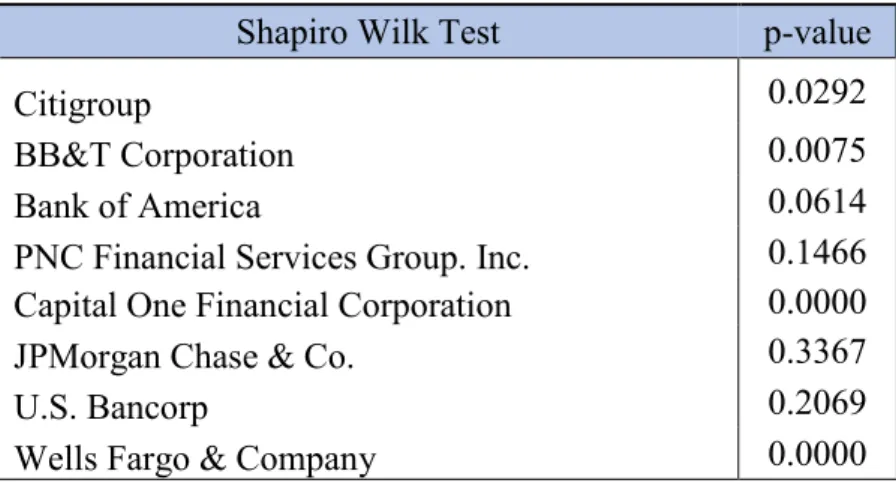
The state variable, 𝛿, in this dissertation is defined as the sum of the earnings before taxes and the banks' operational fixed costs. The earnings before taxes used in this dissertation are proxied
by the net income before taxes. As further mentioned, the banks’ operational fixed costs are proxied by using the non-interest expenses of the banks. The GJL (2001)-model implies an assumption that the dynamics of the state variable follow a geometric Brownian motion. This assumption implies that their log changes follow a normal distribution. To test this, we are applying a Shapiro-Wilk test in the program R. The significance level we are testing for is chosen for an alpha level of 0.05 and therefore a p-value of less than 0.05 signals a rejection of the null hypothesis, which is that the data is normally distributed. For a p-value higher than 0.05 we don’t reject the null hypothesis, which does not mean that the data is not normally distributed (we just can’t reject that hypothesis).
Table 3 – Shapiro-Wilk Test for Normality
Shapiro Wilk Test p-value
Citigroup 0.0292
BB&T Corporation 0.0075
Bank of America 0.0614
PNC Financial Services Group. Inc. 0.1466
Capital One Financial Corporation 0.0000
JPMorgan Chase & Co. 0.3367
U.S. Bancorp 0.2069
Wells Fargo & Company 0.0000
The null hypothesis can be accepted for the Bank of America, Capital One, JPMorgan Chase, U.S. Bancorp that the dynamics of their state variables follow a normal distribution. Followingly, we reject the test for normal distribution in the cases of Citigroup, BB&T, PNC and Wells Fargo & Co and conclude therefore that their state variables are not normally distributed.
Also, the skewness of the companies' state variables was analysed. A negative skewness normally refers to a longer or “fatter” tail on the left side of the distribution, while a positive skewness refers to a longer or fatter tail on the right side. Financial institutions prefer a negative skewness, due to the small amount of very high outliers and the majority of smaller values. Therefore, the skewness retrieves information about the extreme values in comparison to one and the other tail. The skewness of the companies’ state variable is presented in the following table:
Table 4 – Skewness of companies’ state variable
C BBT BAC COF PNC JPM USB WFC
It is to see that the state variables of Citigroup, U.S. Bancorp and JPMorgan Chase have the largest negative skewness and therefore they are most likely to suffer from the largest decreases in values. Nevertheless, negative skewness is preferred due to the likelihood of frequent gains and only a few large losses.
Further, the kurtosis of the state variables was analysed as well to retrieve further information about the distribution of the latter. The information that can be observed are the extreme values in either tail. Means that a low kurtosis displays fewer extreme values, while a high kurtosis displays higher extreme values. The results are presented in the following table:
Table 5 – Kurtosis of the companies’ state variable
C BBT BAC COF PNC JPM USB WFC
5.20 1.94 2.05 1.60 1.21 1.50 2.18 1.22
Following these results, it is to say, that Citigroup, Bank of America, and BB&T are going to suffer the most extreme values in their state variables.
Equity value
In this dissertation, we assume to know the equity value from retrieving the market value of the companies in the sample. The data got retrieved from the Thomson Reuters Data stream platform.
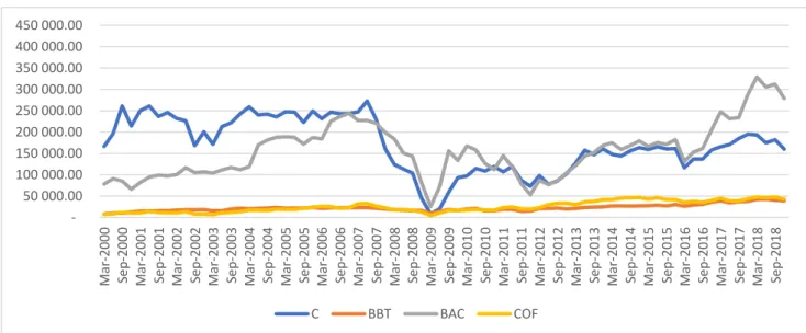
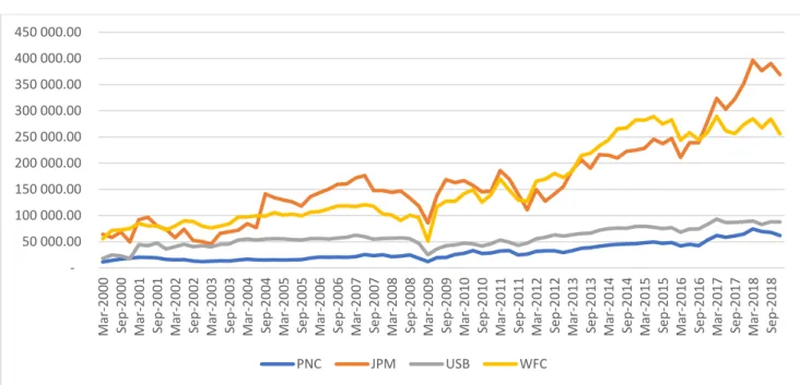
Figure 1 – Quarterly Equity Values (in millions $)
50 000.00 100 000.00 150 000.00 200 000.00 250 000.00 300 000.00 350 000.00 400 000.00 450 000.00 Mar-2000 Se p -2000 Mar-2001 Se p -2001 Mar-2002 Se p -2002 Mar-2003 Se p -2003 Mar-2004 Se p -2004 Mar-2005 Se p -2005 Mar-2006 Se p -2006 Mar-2007 Se p -2007 M ar -20 08 S e p -20 08 Mar-2009 Se p -2009 Mar-2010 Se p -2010 Mar-2011 Se p -2011 Mar-2012 Se p -2012 Mar-2013 Se p -2013 Mar-2014 Se p -2014 Mar-2015 Se p -2015 Mar-2016 Se p -2016 Mar-2017 Se p -2017 Mar-2018 Se p -2018 C BBT BAC COF
Figure 2 – Quarterly Equity Values (in millions $)
The market value is defined as the share price multiplied by the number of ordinary shares issued. Therefore, it is to see that all financial institutions perceived major declines within their equity values throughout the financial crisis of 2007 – 2008. The largest losses in their market capitalization were observed for Citigroup, Bank of America, and JPMorgan Chase. Even though, these declines are a signal that shareholders “flee” to quality investments and can indicate future solvency risk (Gray and Jobst, 2010).
Equity Risk Premium (EQRP)
The equity risk premium mentioned previously got retrieved from the website of Professor Damodaran. He started collecting, cleaning and publishing individual company data on his website since the late 1990s to make it available for public use. One of the estimates that is going to be applied in this dissertation is the Free Cash Flow to Equity (FCFE) method. This valuation method is following two slightly different approaches. Their difference can be found within the sustainability of the payout, which can affect the growth rate and their overall levels over time. Due to a lack of data for the year 2000 data is retrieved for this case in a different way. For these missing years, the equity risk premium is assumed to be the implied premium derived from FCFE, for the rest the implied premium from FCFE with sustainable payout is taken into consideration. Applying this data resolved that the implied premium from FCFE contains lower rates for the missing years, which decrease the prediction of the default probabilities. 50 000.00 100 000.00 150 000.00 200 000.00 250 000.00 300 000.00 350 000.00 400 000.00 450 000.00 Mar-2000 Se p -2000 Mar-2001 Se p -2001 Mar-2002 Se p -2002 Mar-2003 Se p -2003 Mar-2004 Se p -2004 Mar-2005 Se p -2005 Mar-2006 Se p -2006 Mar-2007 Se p -2007 M ar -20 08 S e p -20 08 Mar-2009 Se p -2009 Mar-2010 Se p -2010 Mar-2011 Se p -2011 Mar-2012 Se p -2012 Mar-2013 Se p -2013 Mar-2014 Se p -2014 Mar-2015 Se p -2015 Mar-2016 Se p -2016 Mar-2017 Se p -2017 Mar-2018 Se p -2018 PNC JPM USB WFC
Figure 3 – Historical Free Cashflow to Equity comparison
Historical Betas (𝛽)
To compute the market price of risk, it is necessary to retrieve the historical betas of the companies of the sample. These beta coefficients are a measure of systemic risk. Therefore, they enable us to look at time periods of increased volatility and exposure to the market. The quarterly beta coefficients of the companies are presented in the following figure:
Figure 4 – Historical Beta Coefficients 𝛽
Substantially it is to say that the historical beta coefficients vary in their value, but they are 0.00% 1.00% 2.00% 3.00% 4.00% 5.00% 6.00% 7.00% 8.00% 9.00% 2000 2001 2002 2003 2004 2005 2006 2007 2008 2009 2010 2011 2012 2013 2014 2015 2016 2017 2018
Implied Premium (FCFE) Implied Premium (FCFE with sustainable Payout)
0.00 0.50 1.00 1.50 2.00 2.50 3.00 3.50 M ar -20 00 S e p -2000 Mar-2001 Se p -2001 Mar-2002 Se p -20 02 Mar-2003 Se p -2003 Mar-2004 Se p -2004 M ar -20 05 S e p -2005 Mar-2006 Se p -2006 Mar-2007 Se p -20 07 Mar-2008 Se p -2008 Mar-2009 Se p -2009 M ar -20 10 S e p -2010 Mar-2011 Se p -2011 Mar-2012 Se p -20 12 Mar-2013 Se p -2013 Mar-2014 Se p -2014 M ar -20 15 S e p -2015 Mar-2016 Se p -2016 Mar-2017 Se p -20 17 Mar-2018 Se p -2018
to decrease while the crisis took place. After the crisis, they were increasing again to a pre-crisis level.
Analysing this behaviour, the betas that were taken into consideration here are computed on the basis of a long duration of time, which enables them to return more robust solutions. Further, the fact of the long duration could cause a variation in the results, that is not wanted and therefore we are assuming a constant, average beta for every bank. The constant value gets justified under the assumption that the banks did not change their business model drastically through the time period analysed.
Table 6 – Mean beta coefficient 𝛽
C BBT BAC PNC COF JPM USB WFC
1.60 1.43 1.33 0.89 0.96 0.92 1.43 0.96
Tax Rates
As in the paper published by Goldstein, Ju, and Leland (2001), we assume a constant tax rate
equal to 20% over the whole time. Hence, we assume a 𝑇𝑎𝑥𝑟𝑎𝑡𝑒𝐷𝑖𝑣𝑖𝑑𝑒𝑛𝑑 of 20% and
𝑇𝑎𝑥𝑟𝑎𝑡𝑒𝐶𝑜𝑟𝑝𝑜𝑟𝑎𝑡𝑒 of 20%. This assumption was considered throughout the whole paper and
led to the computation of an effective tax rate of
(1 − 𝑇𝑎𝑥𝑟𝑎𝑡𝑒𝐸𝑓𝑓𝑒𝑐𝑡𝑖𝑣𝑒) = (1 − 𝑇𝑎𝑥𝑟𝑎𝑡𝑒𝐷𝑖𝑣𝑖𝑑𝑒𝑛𝑑) ∗ (1 − 𝑇𝑎𝑥𝑟𝑎𝑡𝑒𝐶𝑜𝑟𝑝𝑜𝑟𝑎𝑡𝑒),
which leads up to an effective tax rate of 36% for interest payments to investors. Interest rate (RF)
The interest rate used in this dissertation is the 30-year U.S. treasury bond bid rate. This rate is decreasing over time. As we want to measure the effect of taxes on the whole company process it is necessary to reduce the interest rate by the effective tax rate, which enables us to retrieve following interest rate over the time span.
Figure 5 – Interest rate
Historical equity volatility 𝜎𝑒
The volatility of the equity, 𝜎𝑒, got empirically computed with the program R. Therefore, the
standard deviation of the difference of the log changes of the equity was taken into consideration. Further, the sample size got cleaned from outliers by setting upper and lower limits of three standard deviations as boundary conditions. To annualize the results, due to the usage of weekly data, got annualized by multiplying them by the square root of 52.
Table 7 – Annualized equity volatility σ_e
C BBT BAC PNC COF JPM USB WFC
35.27% 25.92% 34.58% 26.78% 38.35% 31.23% 26.20% 25.83% This table provides information about the financial institutions with the highest and lowest volatile equities. COF and C show high volatility of more than 35%, while WFC and BBT possess the lowest volatility of around 26%. Regarding the regular definition of volatility, the companies with the highest volatilities are meant to be the ones with the highest risk related to the size of changes in their assets.
Expected rate of return for equity 𝜇𝑒
Further, the CAPM parameters were used to compute the expected rate of return of the equity of the financial institutions. These were calculated as mentioned in section 4.2.2. Computation
0.00% 0.50% 1.00% 1.50% 2.00% 2.50% 3.00% 3.50% 4.00% 2000 2001 2002 2003 2004 2005 2006 2007 2008 2009 2010 2011 2012 2013 2014 2015 2016 2017 2018
of market price risk. Further, the expected rate of return for equity is used as an auxiliary function to compute the market price of risk.
Table 8 – Average expected rate of return on equity 𝜇𝑒
C BBT BAC COF PNC JPM USB WFC
11.98% 8.50% 11.03% 11.05% 8.32% 10.43% 8.52% 8.04% The CAPM parameters of interest rate and the equity risk premium proposed by Damodaran are the same for each bank, due to the same geographic location and at the same time. Therefore, the only difference in this computation is the beta coefficient. Due to these similarities in the inputs the pure effect of risk that an investment is adding to the portfolio can be observed in the different average expected returns.
Market price of risk 𝜃
Further, we analysed the market price of risk by using equation 27. First of all, we computed the mean market price of risk.
Table 9 – Mean market price of risk 𝜃
C BBT BAC PNC COF JPM USB WFC
24.14% 19.47% 21.87% 18.14% 19.79% 22.32% 19.29% 17.71% The result of the market price of risk retrieved from the companies’ data was taken into consideration by computing the mean of it. That was done because the dataset only contains companies from the same sector, which includes similarity in the behaviour of the market price of risk in times of crisis. Therefore, it can also be seen as a risk-to-reward ratio for a market portfolio. The companies with the highest mean market price of risk are Citigroup, Bank of America, JPMorgan Chase, and BB&T.
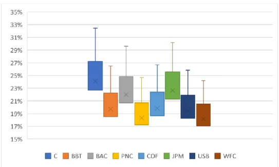
Further, the market price of risk got analysed by displaying the results in a boxplot graph form. This provided further evidence about outliers, minimal and maximal values, and the mean of the market price of risk. These results can be observed in the Figures 6.
Figure 6 – Market price of risk boxplot
As shown in Table 9, the means of the market price of risk differ a lot over the sample. Overall, we can conclude that the banks market price of risk tends to be affected a lot by the time series of beta. The difference in the shapes of the boxplots can be explained by differences in the historical equity volatility as well. The significant differences between the equity volatilities cause the variation in the shape of the boxplots. Further, we are analysing the time series results of the market risk premium and observe it for in- and decreases.
Figure 7 – Panel A (Market price of risk)
0% 5% 10% 15% 20% 25% 30% 35% 40% Mar-2000 Se p -2000 Mar-2001 Se p -2001 Mar-2002 Se p -2002 Mar-2003 Se p -2003 Mar-2004 Se p -2004 Mar-2005 Se p -2005 Mar-2006 Se p -20 06 Mar-2007 Se p -2007 Mar-2008 Se p -2008 Mar-2009 Se p -2009 Mar-2010 Se p -2010 Mar-2011 Se p -2011 Mar-2012 Se p -2012 M ar -20 13 S e p -2013 Mar-2014 Se p -2014 Mar-2015 Se p -2015 Mar-2016 Se p -2016 Mar-2017 e S p -2017 Mar-2018 Se p -2018 C BBT BAC PNC
Figure 8 – Panel B (Market price of risk)
Figure 7 and 8 provide information about the dynamics of the market price of risk for the corresponding banks. It can be observed that the market price of risk for all banks are sinking in times of crisis and after these occur, they tend to increase again. These changes are mainly caused by the time series changes of the equity risk premium as they move similarly. As stated above, the previous variation through the time series of the betas was cleaned by using an average beta.
4.2.2 Iteratively obtained variables
This section is determined to the variables that got obtained from the iterative approach
mentioned in chapter 4.1.1. These variables are the annualized volatility of the project 𝜎𝑣 and
the payout ratio k.
Annualized volatility of the project 𝜎𝑣
Table 10 – Projects volatility σ_v
C BBT BAC PNC COF JPM USB WFC
20.50% 17.97% 22.20% 17.49% 21.43% 20.91% 22.61% 18.04%
In comparison to the historical equity volatility, 𝜎𝑒, it is to say that the projects volatility, 𝜎𝑣,
is significantly lower in all cases, which can be explained through the naturally higher volatility of equity, when its defined as the market capitalization. As the market capitalization suffered
0% 5% 10% 15% 20% 25% 30% 35% 40% Mar-2000 De c-2000 S e p -2001 Ju n -2002 Mar-2003 De c-2003 S e p -2004 Ju n -20 05 Mar-2006 De c-2006 S e p -2007 Ju n -2008 Mar-2009 De c-2009 S e p -2010 Ju n -2011 Mar-2012 De c-2012 S e p -2013 Ju n -2014 Mar-2015 De c-2015 S e p -2016 Ju n -20 17 Mar-2018 De c-2018 COF JPM USB WFC
from significant decreases the higher rates can be explained through this. Another reason could be that the project volatility got modelled by implying the operational leverage.
Further there was a positive correlation between the volatility of the equity and the asset volatility observed.
Payout ratio k
Table 11 – Payout ratio for each company
C BBT BAC PNC COF JPM USB WFC
3.00% 2.68% 3.15% 2.74% 3.32% 3.12% 2.44% 2.79%
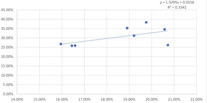
The payout ratios k found within the financial sector of the United States contains similar values over the whole data sample. Even though there have been banks that have been hit by the financial crisis their payout ratios overall are similar to the ones that were hit less. In GJL (2001)’s paper, they state that there is a positive correlation between the level of C and the value for the payout ratio k, which tends to be not the case. Typically, a lower level of k can be found in companies that are reinvesting their earnings into growing business, research, or further developments. Overall, a positive and stable payout ratio is important for companies to indicate shareholders that the company is knowing about their risk and reducing it. Further, the reduction of default risk, through good risk management can lead to higher future payout ratios, which are then priced by the market by stock acquisitions, which was found by Charitou and Lambertides (2011). y = 1.5095x + 0.0256 R² = 0.3342 0.00% 5.00% 10.00% 15.00% 20.00% 25.00% 30.00% 35.00% 40.00% 45.00% 14.00% 15.00% 16.00% 17.00% 18.00% 19.00% 20.00% 21.00% 22.00%
5. Results
This chapter has two sections. The first section discusses the values obtained for the distance-to-default and the probability of default and explores the roots behind these results. The second section compares the obtained results with the ones implied by the credit ratings given by two of the most important rating agencies: Moody’s and S&P.
5.1 Credit Risk Indicators
This section presents the credit risk metrics that were computed in this dissertation. These metrics were the default barrier-to-asset ratio, the drift of the process, the distance-to-default (DD) and the probabilities of default.
5.1.1 Default barrier-to-asset ratio
The barrier-to-asset ratio tells how far the bank is from default at a given moment in time. As such, it can be interpreted as a measure of leverage. The barrier-to-asset ratio is always lower than 1. The closer this ratio is to 1 the closer the company is to default. Differently from the distance-to-default, the barrier-to-asset ratio does not adjust for risk. Figure 9 and 10 show the barrier-to-asset ratio for the eight banks considered in this dissertation. The ratios range from 14.55% to 71.38%. For most of the banks the maximum value was obtained between Q1 and Q3 of 2009, while three banks obtained values above 50%. These three were Citigroup (71.38%), the Bank of America (51.37%), and Capital One (51.01%). The yearly results are presented in Appendix 5.
Figure 9 – Default barrier-to-asset ratio
Figure 10 – Default barrier-to-asset ratio
5.1.2 Drift of the process 𝜇𝑝
The drift of the process tells us the expected growth rate of the project value. It is defined as
the difference between the expected return from the project 𝜇𝑣 and the payout ratio 𝑘. Figure
11 and 12 show the drift of the process. The drift ranges from 1.82% to 7.83%, while the average drift is 4.72%. The most banks obtained their maximum value in Q2 2011. Meanwhile the minimum value for the most banks were obtained in Q3 2016. As the market price of risk, the payout ratio and the project volatility are constant variables in this computation, its dynamics
0.00% 10.00% 20.00% 30.00% 40.00% 50.00% 60.00% 70.00% 80.00% Mar-2000 Se p -2000 M ar -20 01 S e p -2001 Mar-2002 Se p -2002 Mar-2003 Se p -2003 Mar-2004 Se p -2004 Mar-2005 Se p -2005 Mar-2006 Se p -2006 Mar-2007 Se p -2007 Mar-2008 Se p -2008 Mar-2009 Se p -2009 Mar-2010 Se p -2010 Mar-2011 Se p -2011 Mar-2012 Se p -2012 Mar-2013 Se p -2013 M ar -20 14 S e p -2014 Mar-2015 Se p -2015 Mar-2016 Se p -2016 Mar-2017 Se p -20 17 Mar-2018 Se p -2018 C BBT BAC PNC 0.00% 10.00% 20.00% 30.00% 40.00% 50.00% 60.00% 70.00% 80.00% Mar-2000 Se p -2000 M ar -20 01 S e p -2001 Mar-2002 Se p -2002 Mar-2003 Se p -2003 Mar-2004 Se p -2004 Mar-2005 Se p -2005 Mar-2006 Se p -2006 Mar-2007 Se p -2007 Mar-2008 Se p -2008 Mar-2009 Se p -2009 Mar-2010 Se p -2010 Mar-2011 Se p -2011 Mar-2012 Se p -2012 Mar-2013 Se p -2013 M ar -20 14 S e p -2014 Mar-2015 Se p -2015 Mar-2016 Se p -2016 Mar-2017 Se p -20 17 Mar-2018 Se p -2018 COF JPM USB WFC
implies that the banks are expected to deleverage over time. The yearly drifts of the process are presented in Appendix 7.
Figure 11 – Drift of the process 𝜇𝑝
Figure 12 – Drift of the process 𝜇𝑝
5.1.3 Distance-to-Default (5-year)
Figures 13 and 14 present the distance-to-default for the 8 banks considered. On average the distance-to-default is 3.16. The bank with the lowest average value is Citigroup (0.98) and the one with the highest average value is BB&T (2.62). The yearly distance-to-default values for all companies are presented in Appendix 6.
0% 1% 2% 3% 4% 5% 6% 7% 8% 9% Mar-2000 Se p -2000 Mar-2001 Se p -2001 Mar-2002 Se p -2002 Mar-2003 Se p -2003 Mar-2004 Se p -2004 M ar -20 05 S e p -2005 Mar-2006 Se p -2006 Mar-2007 Se p -2007 Mar-2008 Se p -2008 Mar-2009 Se p -2009 Mar-2010 Se p -2010 Mar-2011 Se p -2011 Mar-2012 Se p -2012 Mar-2013 Se p -2013 Mar-2014 Se p -2014 Mar-2015 Se p -20 15 Mar-2016 Se p -2016 Mar-2017 Se p -2017 Mar-2018 Se p -2018 C BBT BAC PNC 0% 1% 2% 3% 4% 5% 6% 7% 8% 9% Mar-2000 Se p -2000 Mar-2001 Se p -2001 Mar-2002 Se p -2002 Mar-2003 Se p -2003 Mar-2004 Se p -2004 M ar -20 05 S e p -2005 Mar-2006 Se p -2006 Mar-2007 Se p -2007 Mar-2008 Se p -2008 Mar-2009 Se p -2009 Mar-2010 Se p -2010 Mar-2011 Se p -2011 Mar-2012 Se p -2012 Mar-2013 Se p -2013 Mar-2014 Se p -2014 Mar-2015 Se p -20 15 Mar-2016 Se p -2016 Mar-2017 Se p -2017 Mar-2018 Se p -2018 COF JPM USB WFC
Figure 13 – Quarterly DD of companies
Figure 14 – Quarterly DD of companies
The smallest distance-to-default was found for Citigroup, in March 2009 with a value of 0.98. Further, the Bank of America was analysed to have the second-lowest value with 1.53 on the same date. The third lowest value of 1.54 for the data sample got retrieved for Capital One
Financial Corp. on the 13th of March 2009. The distance-to-default for all banks are highly
correlated with an average correlation value of 85.69%. This high level of correlation results from the high correlation observed in stock prices. Further, this could result from “similar” asset volatilities retrieved from the iterative approach. Through their similar values in a range from 17.49% to 22.61%, the difference in the distance-to-default’s most likely occurs through different default points, the asset values, and the drifts. Overall, the distance-to-default captures
0 1 2 3 4 5 6 Mar-2000 Se p -2000 Mar-2001 Se p -2001 Mar-2002 Se p -2002 Mar-2003 Se p -2003 Mar-2004 Se p -2004 Mar-2005 Se p -2005 Mar-2006 Se p -2006 Mar-2007 Se p -2007 Mar-2008 Se p -2008 Mar-2009 Se p -2009 Mar-2010 Se p -2010 Mar-2011 Se p -2011 Mar-2012 Se p -2012 Mar-2013 Se p -2013 Mar-2014 Se p -2014 Mar-2015 Se p -2015 Mar-2016 Se p -2016 Mar-2017 Se p -2017 Mar-2018 Se p -2018 C BBT BAC PNC 0 1 2 3 4 5 6 Mar-2000 Se p -2000 Mar-2001 Se p -2001 Mar-2002 Se p -2002 Mar-2003 Se p -2003 Mar-2004 Se p -2004 Mar-2005 Se p -2005 Mar-2006 Se p -2006 Mar-2007 Se p -2007 Mar-2008 Se p -2008 Mar-2009 Se p -2009 Mar-2010 Se p -2010 Mar-2011 Se p -2011 Mar-2012 Se p -2012 Mar-2013 Se p -2013 Mar-2014 Se p -2014 Mar-2015 Se p -2015 Mar-2016 Se p -2016 Mar-2017 Se p -2017 Mar-2018 Se p -2018 COF JPM USB WFC
information about the distance-of-the assets from the barrier, which monitors leverage. Further, information regarding the risk through the volatility of the assets, and the expected change in leverage through the drift.
5.1.4 Probabilities of default (5-years)
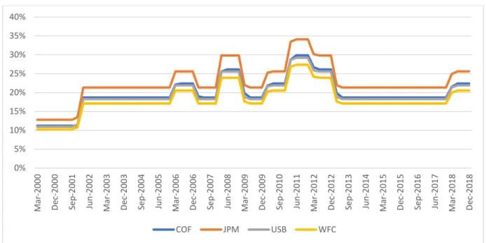
The probabilities of default that got retrieved from applying the model on the banking sector are the core element of this dissertation. Further, the probabilities were computed as 5-year probabilities of default. All calculations were done on weekly frequency. This was important to better estimating the model parameters. For simplicity, we decided however to present quarterly graphs, while mentioning peaks in a weekly frame. In addition, yearly results are presented in Appendix 4. Figure 15 and Figure 16 present the probabilities of default in a quarterly timeframe.
Figure 15 – Quarterly probabilities of default
0.00% 5.00% 10.00% 15.00% 20.00% 25.00% 30.00% 35.00% 40.00% 45.00% Mar-2000 Se p -2000 Mar-2001 Se p -20 01 Mar-2002 Se p -2002 Mar-2003 Se p -2003 Mar-2004 Se p -2004 Mar-2005 Se p -2005 Mar-2006 Se p -2006 Mar-2007 Se p -2007 Mar-2008 Se p -2008 Mar-2009 Se p -2009 Mar-2010 Se p -2010 Mar-2011 Se p -2011 M ar -20 12 S e p -2012 Mar-2013 Se p -2013 Mar-2014 Se p -2014 Mar-2015 Se p -2015 M ar -20 16 S e p -2016 Mar-2017 Se p -2017 Mar-2018 Se p -2018 C BBT BAC PNC