UNIVERSIDADE DE LISBOA
FACULDADE DE CIÊNCIAS
DEPARTAMENTO DE ENGENHARIA GEOGRÁFICA, GEOFÍSICA E ENERGIA
Study and Characterization of the Impacts of Soiling on the
Performance of Photovoltaic Systems
Francisco Pile Mendes Pinto
Mestrado Integrado em Engenharia da Energia e do Ambiente
Dissertação orientada por:
Anne Migan (GEEPS)
Acknowledgements
I would like to express my gratitude towards my parents for their unconditional love and encouragement, patiently assisting me on the completion of my studies.
I am also profoundly grateful to Anne Migan, without whom this work would not have been possible, and whose tireless support proved instrumental throughout this project.
I would like to acknowledge Vincent Bourdin and Jordi Badossa for their invaluable guidance, criticism, friendship and optimism, as well as for their continuous availability and assistance in any of the numerous challenges I’ve encountered.
Finally, my sincerest appreciation goes to Elsa Heyd for her companionship, advice, and illuminating views on a number of issues related to the project.
Preface/Motivation
The accumulation of particles on the surface of solar panels is an important factor affecting solar panel production. This phenomenon, commonly referred to as soiling, can amount to a sizeable portion of the system losses. Despite this, perhaps due to its inevitability, soiling losses remain largely overlooked. It’s for this reason that I’m particularly interested in understanding and quantifying soiling related losses, aiming to determine the extent of their impact on photovoltaic systems and their conversion efficiency. Although several studies have been published on this subject, few analyzed soiling through the correlation between efficiency and rain, a much more accessible method for those without the time or means to more accurately assess soiling losses.
This study is aimed at all those who seek to understand how soiling affects the conversion efficiency of photovoltaic systems, and particularly at those interested on its impact on modules located close to the region of Paris, where this study was performed.
Abstract
Soiling can be one of the major causes of power loss on photovoltaic systems. Despite this, these remain largely ignored. This study analyzed the soiling-induced efficiency degradation of five different solar modules, aiming to characterize and quantify the impact of soiling on the performance of these systems. This was accomplished through the analysis of the module efficiencies over dry periods, during which rain was insufficient to effectively clean the panels. Results showed that all panels registered an efficiency decrease within a ninety percent confidence interval during the longest dry period, with an average power degradation rate of -0.042 %/Day, suggesting a stable trend of soiling induced efficiency degradation. All other periods exhibited non-significant trends, likely due to the high day-to-day efficiency fluctuations which persisted despite the thermal correction of the efficiency values. The accuracy of two thermal models was tested, aiming to obtain the most reliable module temperature records to be employed in the thermal correction procedure. The first, already existent in the literature and based on the panels’ NOCT yielded the best results, with an average error of 3.55 ºC. The second, based on the precise modelling of the panels’ heat fluxes, proved less practical and reliable, yielding a slightly average error in the order of 3.9 ºC. Finally, the impact of the diffuse radiation on the dispersion of the daily efficiency values was studied, revealing that the latter is proportional to the diffuse ratio. This was achieved through the analysis of the monthly standard deviation for different day types, so as to bypass the effect of seasonal variations. Results suggest that solar panel cleaning can be neglected in the region of Palaiseau, as soiling losses are rendered insignificant due to the combination of moderate panel inclinations and the natural cleaning provided by the high frequency of rainfall events.
Resumo
A acumulação de partículas na superfície de painéis solares é um fenómeno transversal a todas as tecnologias fotovoltaicas. Este fenómeno é designado por Soiling, e têm como principal consequência a redução da eficiência fotovoltaica dos painéis.
Esta tese tem como por objetivo a caracterização e quantificação das perdas causadas pelo efeito do soiling em painéis solares. Para tal, serão estudados cinco módulos instalados nos arredores de Paris com o intuito de obter uma taxa de degradação da potência para cada painel.
O impacto do Soiling será estudado através da análise da eficiência dos painéis durante períodos secos, com um foco especial no maior período seco de que existem registos, durante o qual todos os módulos sofreram um decréscimo de eficiência para um intervalo de confiança superior a noventa por cento. Os painéis encontram-se no Observatório SIRTA [1], orientados a Sul a uma inclinação fixa de vinte e sete graus. Situados em terreno aberto, a cerca de vinte centímetros do solo, os painéis estão inseridos numa área rodeada por extensos relvados, caracterizada por uma fraca intensidade rodoviária.
Para a realização deste estudo, foi disponibilizada uma ampla gama de dados amostrados em intervalos de dez minutos, permitindo uma precisa análise intra-diária da eficiência fotovoltaica. Dados como a temperatura, potência, corrente e tensão dos painéis, irradiância, temperatura ambiente, pluviosidade, velocidade do vento, humidade relativa, entre muitos outros, possibilitaram não só o estudo do impacto do soiling na performance dos painéis, como também várias outras análises acessórias relevantes. A tese inicia-se por uma abordagem aos principais fatores que afectam a taxa de deposição de partículas nos módulos, assim como os seus variados impactos na eficiência dos painéis. Esta secção visa introduzir o leitor aos conceitos básicos indispensáveis à compreensão da tese, e igualmente fornecer uma contextualização alargada de modo a facilitar a interpretação dos resultados apresentados.
Seguem-se depois os métodos e objetivos, o capítulo central desta tese, o qual explica em detalhe todo o processo que culminou na quantificação do impacto do soiling na performance dos painéis estudados. Este capítulo encontra-se dividido em aproximadamente três partes. A primeira, relativa ao processamento inicial dos dados, envolve o cálculo da temperatura dos módulos, a sua eficiência de conversão e subsequente correção térmica. Grande parte desta seção é dedicada estimação das temperaturas dos módulos, as quais serão necessárias para preencher eventuais lacunas devido a falhas dos sensores térmicos.
Estas temperaturas serão obtidas através da implementação de dois modelos térmicos capazes de simular a temperatura dos módulos. O primeiro, já existente na literatura, requer apenas a introdução da temperatura ambiente, irradiância, e a temperatura nominal de operação das células solares. Embora este valor seja geralmente fornecido pelo fabricante, este último foi calculado experimentalmente, assegurando que o modelo fosse fornecido com temperaturas nominais de operação de células reais, medidas nas suas verdadeiras condições de operação.
O segundo modelo, baseado na modelação /dos fluxos de calor entre o painel e o ambiente, foi criado de raiz com o intuito de aumentar a precisão das estimativas. A estabilidade e desempenho destes modelos será avaliada, comparando a sua precisão e fiabilidade sob diferentes condições.
De seguida, a eficiência dos painéis será calculada e corrigida para uma temperatura base de vinte e cinco graus Celcius. Esta correção é indispensável à análise da degradação do desempenho dos painéis,
de potência normalizadas. A qualidade desta correção será também estudada de modo a garantir a validade dos resultados.
O segundo passo centra-se no reprocessamento dos valores de eficiência por forma a facilitar a deteção de eventuais perdas, permitindo obter uma taxa de degradação da potência fiável. Para tal, a eficiência diária acumulada dos painéis será calculada, com o objetivo de simplificar a análise através da redução das variações intra-diárias, obtendo uma série mais representativa das variações de eficiência. Nesta fase serão também filtrados valores anormais de eficiência, resultantes de erros de medição ou condições de fraca iluminação, detrimentais ao estudo em curso.
Será ainda feita uma análise da relação entre a dispersão dos valores diários de eficiência e as condições climatéricas, uma vez que estas podem dificultar a análise dos impactos do soiling, afetando a extração e significância estatística das taxas de degradação de eficiência.
O terceiro e último passo consiste na identificação dos períodos secos, ou intervalos durante os quais a chuva não foi suficientemente forte por forma a interferir com a acumulação de partículas nos painéis, e portanto ideais para o cálculo das taxas de degradação da eficiência. Estas serão baseadas no declive da recta resultante de uma regressão linear das eficiências durante estes períodos.
O uso de uma regressão linear na previsão de perdas pelo efeito do soiling é baseado em estudos de natureza semelhante, os quais concluíram que o declínio do desempenho fotovoltaico observado durante períodos secos é aproximadamente linear, decrescendo continuamento durante períodos sem chuva e regressando a níveis normais após um episódio de precipitação [2]. Estes factos sugerem que os efeitos do soiling no desempenho de um Sistema PV podem ser estimados adotando um modelo linear de perdas de eficiência entre eventos significativos de precipitação.
A quantificação destas perdas foi feita para dois tipos de períodos. Inicialmente, apenas períodos durante os quais a precipitação diária não excedeu os cinco milímetros foram estudados. Isto consistiu no cálculo das taxas de degradação da eficiência para estes intervalos. De seguida, este limiar foi fixado num valor mais conservador, assegurando que nenhum processo de limpeza possa ter acontecido, e as taxas de degradação recalculadas.
Uma ênfase especial foi dada ao mais longo período seco de que existem registos, durante o qual todos os painéis registaram uma diminuição inequívoca de eficiência. A taxa de degradação média de potência durante este intervalo foi de -0.042 %/Dia, um valor que se encontra de acordo com vários outros estudos semelhantes [2,3]. Devido à sua incomparável duração, estendendo-se por trinta e sete dias, uma especial atenção foi dada a este intervalo, uma vez que este foi o mais longo período de acumulação ininterrupta de partículas.
Por fim, foi feita uma breve análise estatística das regressões lineares, visando validar os resultados. As regressões lineares foram testadas unidireccionalmente, de modo a determinar a probabilidade de um painel registar um decréscimo de eficiência durante este período. Para tal, foram calculados os intervalos de confiança de cada regressão baseados na distribuição t de student, focando-se exclusivamente no intervalo superior, revelando o revelando o nível de confiança com o qual se pode afirmar que perdas devidas ao efeito do soiling estão presentes em cada painel.
Os resultados indicaram que todos os painéis sofreram uma queda de eficiência para um intervalo de confiança superior a noventa porcento durante este período mais longo, e de noventa e cinco por cento para quatro dos painéis.
Table of Contents
Acknowledgements ... i
Preface/Motivation ... ii
Abstract ...iii
Resumo ... iv
List of Figures and Tables ... viii
List of Acronyms ... x
Chapter 1 – Introduction ... 1
Chapter 2 – Theoretical Background ... 2
2.1. What is Soiling? ... 2
2.2. Causes ... 2
2.3. Atmospheric Parameters Influencing the Rate of Soiling... 2
2.3.1. Rainfall ... 3
2.3.2. Wind ... 3
2.3.3. Humidity ... 4
2.4. Main Parameters Affecting Soiling Deposition and PV Performance ... 4
2.4.1. Deposition Density ... 4 2.4.2. Installation Design ... 5 2.4.3. Incidence Angle ... 5 2.4.4. Dust properties ... 6 2.4.5. Air Mass ... 6 2.4.6. Spectral Composition... 7 2.4.7. Temperature ... 8
2.4.8. Surface Coating and Rugosity ... 8
2.4.9. Shading ... 8
2.4.10. Natural and Artificial Cleaning ... 9
Chapter 3 – Objectives ... 10
Chapter 4 – Methods ... 11
4.1. Calculation of Module Temperature ... 12
4.1.1. NOCT Thermal Model... 12
4.1.2. HEAT Thermal Model ... 21
4.1.3. Model Testing and Validation ... 31
4.2. Efficiency Calculation ... 39
4.4. Analysis of the Quality of the Temperature Correction ... 44
4.5. Efficiency Processing and Outlier Removal ... 46
4.6. Analysis of the Efficiency Degradation during Dry Intervals... 48
4.6.1. Study Period Selection and Cleaning Threshold ... 49
4.6.2. Implementation of the Linear Regressions ... 50
4.7. Analysis of the Efficiency Degradation during Pollution Peaks ... 60
Chapter 5 - Diffuse Ratio and Module Efficiency ... 64
Chapter 6 – Conclusions and Future Work ... 69
Annex ... 70
List of Figures and Tables
Figure 1: NOCT determination procedure (Sharp) ... 14
Figure 2: Confidence bands and prediction intervals for the NOCT regression (Sharp) ... 15
Figure 3: Confidence bands and prediction intervals for the NOCT regression (France Watts) ... 16
Figure 4: Measured and estimated temperature curves (France Watts) ... 19
Figure 5: Measured and estimated module temperatures over a day with a narrow ambient temperature variation (Sharp) ... 20
Figure 6: Measured and estimated module temperatures over a day with low irradiance ... 21
Figure 7: Radiative Input of the HEAT model (France Watts) ... 23
Figure 8: Radiative output of the HEAT Model (France Watts) ... 24
Figure 9: Convective Output of the HEAT Model (France Watts) ... 25
Figure 10: Electric Output of the HEAT Model (France Watts) ... 26
Figure 11: Optimization of the single parameter convection model (France Watts) ... 27
Figure 12: Accuracy comparison between the NOCT and the single parameter convection HEAT model (France Watts) ... 28
Figure 13: Accuracy comparison between the NOCT and HEAT models (France Watts) ... 30
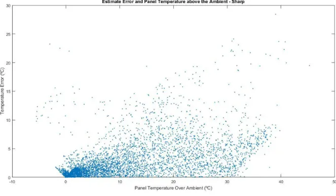
Figure 14: Distribution of the NOCT model’s error with module temperature above the ambient (Sharp) ... 32
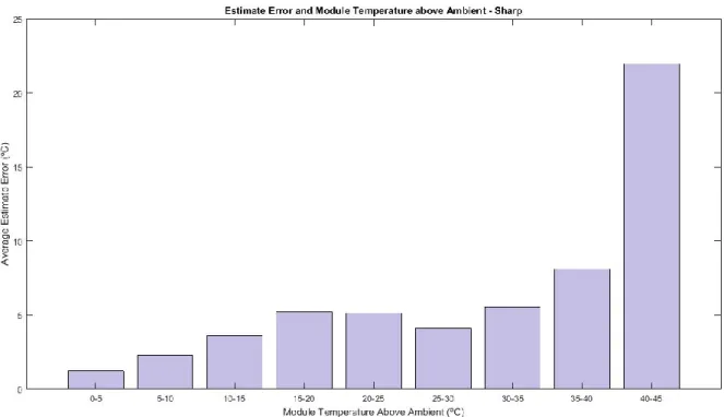
Figure 15: Average NOCT model error with module temperature above ambient (Sharp) ... 33
Figure 16: Average NOCT model error with module temperature above ambient (France Watts) ... 34
Figure 17: Distribution of the module temperatures above ambient (France Watts) ... 35
Figure 18: Relative contribution of each temperature range to the estimate's overall error (France Watts) ... 36
Figure 19: Relative contribution of each temperature range to the estimate's overall error (Sharp) ... 37
Figure 20: Frequency distribution of the estimate's error (France Watts) ... 38
Figure 21: Frequency distribution of the estimate's error (Sharp) ... 39
Figure 22: Module efficiency and temperature over a year and a month (Sharp) ... 40
Figure 23: Efficiency correction procedures: Measured and corrected efficiencies with temperature (Sharp)... 42
Figure 24: Efficiency correction procedures: Measured and corrected efficiencies with temperature (France Watts) ... 43
Figure 25: Variation of module efficiency with temperature over a typical day (France Watts) ... 43
Figure 26: Module efficiency and module temperature (France Watts) ... 45
Figure 27: Filtered and unfiltered histograms of module temperature and efficiency (France Watts) .. 46
Figure 28: Cumulative Daily Efficiency (Sharp) ... 47
Figure 29: Cumulative daily efficiency and rainfall (Sharp) ... 48
Figure 30: Regression lines for all periods with less than five millimetres of rainfall (Sharp) ... 51
Figure 31: Regression lines for all periods with less than five millimetres of rainfall for the remainder of the panels ... 52
Figure 32: Regression lines for the exclusively dry periods during the summer months (Sharp and Frontier) ... 53
Figure 33: Regression lines for all periods with less than zero point two millimetres of rainfall (Sharp) ... 54
Figure 34: Regression lines for all periods with less than zero points two millimetres of rainfall for the remainder of the panels ... 55
Figure 35: Confidence bands and prediction intervals for the regression line of the longest dry interval
(Sharp)... 56
Figure 36: Confidence bands and prediction intervals for the regression lines of the longest recorded dry interval for the remainder of the panels ... 57
Figure 37: Error bars displaying the power degradation values for three confidence levels... 59
Figure 38: Cumulative daily efficiency and periods of peak pollution (France Watts) ... 61
Figure 39: Module Efficiency and PM10 concentration during the first pollution peak (France Watts) ... 62
Figure 40: Interpolation of module efficiency and PM10 concentration during the first pollution Peak (France Watts) ... 62
Figure 41: Interpolation of module efficiency and PM10 concentration during the second pollution peak (France Watts) ... 63
Figure 42: Average monthly diffuse ratio and trendline ... 64
Figure 43: Cumulative daily efficiency and average daily diffuse ratio (Sharp) ... 65
Figure 44: Cumulative daily efficiency and average daily diffuse ratio for the remainder of the panels ... 66
Figure 45: Average monthly standard deviation of the efficiency for each day type (Sharp) ... 67
Figure 46: Average standard deviation of the efficiency for each day type ... 68
Table 1: NOCT model results. Calculated and ideal NOCT values and their respective temperature curve errors. ... 18
Table 2: Prediction error of the NOCT and HEAT models. ... 31
Table 3: Thermal characteristics of the panels. ... 41
Table 4: Summary of the degradation analysis for the longest dry period. ... 57
List of Acronyms
AM Air Mass Coefficient
BNEF Bloomberg New Energy Finance
IEC International Electrotechnical Commission IPSL Institut Pierre Simon Laplace
NOCT Nominal Operating Cell Temperature PM Particulate Matter
PV Photovoltaic
RMSE Root Mean Squared Error
SIRTA Site Instrumental de Recherche par Télédétection Atmosphérique STC Standard Test Conditions
Chapter 1 – Introduction
Over the past two decades the photovoltaic industry has grown exponentially, evolving from a niche market of small-scale applications to a mainstream electricity source.
Solar prices have been dropping at an astonishing rate, consistently ahead of even the most bullish projections. Just three years ago, the Bloomberg New Energy Finance was forecasting solar dropping from 0.53 €/Watt in 2015 to 0.18 €/Watt in 2050. Today, the price already stands between 0.28-0.31€/Watt, and is expected to fall to around 0.20 €/Watt by the end of 2019.
The plunging costs of this technology are the key to its widespread adoption, catering not only to the renewable enthusiasts but to the average consumer as well. With the price per watt falling rapidly, embracing solar is becoming an increasingly economic decision, and not simply an environmentally conscious one.
As the solar PV market grows increasingly competitive, so does the need for accurate energy forecasting in order for this technology to thrive on an industrial scale. An important aspect of this prediction relates to soiling, as it is essential to understand the impacts of soiling in order to properly assess the system’s energy yield.
Soiled solar modules have long been considered a minor nuisance, but with the solar market booming, the proper assessment of soiling losses is becoming increasingly relevant. In recent years, several studies have been conducted by research programs with the goal of assessing the impact of soiling on photovoltaic modules.
On the south of Europe, in Malaga (Spain), a study concluded that the mean daily energy loss along a year caused by dust deposited on the surface of the PV module was around 4.4%, this value increased to 20% during extended periods without rain [4].
Closer to the center of Europe, in Belgium, soiling induced power losses were found to be between 3% and 4%, over a period of just five weeks [5]. In another study, on the island of Crete, yearly power losses were estimated at 5.86% [6]. In the south of Italy, a 6.9% and 1.1% monthly power loss was registered, on plants built on a sandy and a more compact soil, respectively [7].
On the Canary Islands, efficiencies dropped to 20% of their initial values over five months, recovering to their initial values after rainfall [8]. In Kuwait, a notoriously arid climate, soiling losses reached 45.8% over three months without cleaning [9], and in California they amounted to about 7% annually [10]. Other studies report even higher annual yield losses, depending both on system location and the specifications of the analyzed plant.
Despite this, soiling losses are often underestimated, and in part due to the difficulties encountered in their detection. In most cases, the irradiance sensor suffers from the same amount of soil that is covering the PV panels. Consequently, the measured irradiance level decreases, despite the actual irradiance remaining the same. This decrease in the measured irradiance balances out the decrease in the energy production of the panels, allowing for the efficiency to remain constant, and thus effectively hiding the power losses.
But with the increasing number of studies published each year on this subject, the understanding of the impacts of soiling on photovoltaic modules increases, allowing for the development of new techniques
Chapter 2 – Theoretical Background
Over the course of this chapter, there will be an extensive review of the main factors affecting soiling deposition, as well as a brief summary of the key factors related to the impacts of soiling on photovoltaic performance.
2.1. What is Soiling?
Soiling is the phenomenon of dust deposition on the surface of solar panels, resulting in the attenuation of the incoming solar irradiance, and causing a reduction of the modules’ conversion efficiency. This causes PV systems to perform sub-optimally, registering lower efficiencies and generating less power under these conditions. Soiling not only reduces the irradiation on the solar cells, but also the incidence angle of such radiation, further affecting the panel.
These losses can be significantly reduced by a periodical cleansing of the top surface of the solar modules, thus reducing the particle deposition. The ideal time period in-between cleaning depends essentially on the rate of soiling, the type of solar cell technology and the cost of cleaning.
2.2. Causes
There are essentially two interdependent parameters that govern the process of soiling accumulation on solar panels: the local environment and the properties of the soil.
The first defines the rate at which the solar module surface is contaminated, and is directly related to the intensity of the pollution processes and the nature of the prevailing activities. These can be of natural sources, such as pollen, bird droppings and particles brought by the wind, or resultant of human activity, such as combustion products, soot, and rubber dust from nearby road transport.
The second refers to the properties of the soil, which vary with the geographical and atmospheric characteristics of the place, such as with wind, humidity, temperature or pressure, that determine the type, size, weight and shape of the particles.
The physical and chemical properties of such particles are also relevant to determine the effect of soiling on the transmittance of the glass.
There are several other parameters affecting the rate of soiling on a solar panel, such as rainfall, wind speed, orientation, temperature and humidity. These, in conjunction with the environmental characteristics of the location, define the rate of particle deposition on solar modules.
2.3. Atmospheric Parameters Influencing the Rate of Soiling
In this short section, the main atmospheric agents affecting soiling deposition will be covered, providing a summary overview of their impacts.
2.3.1. Rainfall
Rain is an efficient cleaning agent when it occurs frequently and with intensity, as it has the ability to wash away dust particles from a PV module’s surface.
Conversely, light rains tend to drop the suspended particles from the atmosphere, forming thin layers that make PV performance worse. This phenomenon is called wet deposition, and occurs when rain traps air pollutants inside the rain drops and transfers them onto the panel’s surface.
Among all weather variables, rainfall has the highest cleaning potential, allowing for an energy output recovery of up to 99.5% after the modules are cleaned by rain [11].
In the vast majority of the cases, rainfall has a positive effect on PV systems, increasing the transmission coefficient of the glass cover. This is especially true in dry areas where panels can go for months without natural cleaning.
There are, however, some instances in which rain will increase the soiling related losses. In the case of a severely dusted panel, a small amount of rainfall can turn the dust into mud, further promoting dust adhesion and increased soiling deposition.
Similarly, the rain induced transmittance reduction at the lower portion of the glass is more pronounced than at the upper portion, since sometimes rainfall does not clean the sample completely, causing dust from the upper part of the panel to be resettled on the lower part [12].
Finally, it’s worth noting that without proper and regular cleaning, the dust accumulated on the panel’s surface may thicken and not be easily dislodged by rain [13]. Although these cases are rare, requiring manual cleaning in order to restore the panels to their original state, sharp declines in performance have been registered.
2.3.2. Wind
Much like rainfall, wind can be a powerful agent governing the soil deposition process. Whereas strong winds can clear the panel effectively, a slow breeze will often result in dust accumulation. Depending on the geographical location of the solar panels, the wind can act as a serious deposition agent.
In a dry deposition process, wind carries particles until they’re eventually deposited onto PV panel surfaces. This can happen by several means, the most common of which is sedimentation. The orientation of the panels is also marginally relevant to this process, since the dust deposition rate may increase when the panel is facing the wind.
In addition to that, wind velocity also affects the dust sedimentation and deposition characteristics. Dust coatings created by slow winds are less transparent than those created by high speed winds.
between the ripples disappear. This means that the PV module surface is covered by a continuous dust coating, and the surface’s light transmittance is significantly reduced [14].
On the other hand, the removal efficiency of dust by the wind depends on the relative strength of the adhesion forces between surface and particles. Depending on the dust nature, increasing sand accumulation tends to form clusters and upper layers of particles. Under the effect of wind, these clusters will be destroyed but then will resettle on the surface, compared to the single layer particles which will be blown off the surface by the wind. Sand particles tend bounce on the glass surface before settling, hence delaying cluster formation [15].
Finally, the airflow over the panel can have accumulative or dissipative effects at particular places of the module. The air speed and pressure are not constant over the solar panel’s surface, and wherever the airspeed is higher, there will be lower pressure, which can result in lesser soil accumulation and vice versa.
2.3.3. Humidity
When the relative humidity is high, the adhesion of particles to surfaces tends to increase. This means that humidity promotes the adhesion of dust particles onto solar panel surfaces, increasing the soiling rate, and resulting in a more rapid formation of clusters.
Similarly, dew formation due to high relative humidity promotes dust settlement on flat surfaces, while dust adhesion to these surfaces is reinforced by evaporation [13,16].
Furthermore, higher humidity levels lead to capillary forces, creating a bonding bridge between the surface and the contaminant, increasing particle adhesion to surfaces. This means that when contaminated water droplets in fog, mist or clouds come into contact with the panel’s surface, they’re more likely to be deposited.
In a nutshell, the higher the relative humidity in the atmosphere, higher the particle stickiness to the PV panel, and lower the cleansing effect of the wind [17].
2.4. Main Parameters Affecting Soiling Deposition and PV
Performance
2.4.1. Deposition Density
There’s a very clear correlation between dust accumulation and PV performance. This has to do with the fact that the accumulation of dust reduces the transmittance of the solar panel’s glass cover, which in turn reduces the Isc of the system.
As the dust deposition on the glass surface increases, the reduction of the transmission increases at a progressively decreasing rate until its upper limit. When this limit has been reached, the effect of the deposition density on glass transmittance vanishes, remaining constant for higher density levels [18]. Just as the transmissivity of the glass cover, both the Isc and performance decline as the dust deposition
density increases. This Isc degradation rate is higher at initial deposition until a certain level, after which
it decreases only slightly.
The efficiency degradation associated with the loss of transmittance follows an exponential relation with deposition density. However, panel and dust type can govern the degree of efficiency reduction.
2.4.2. Installation Design
The PV installation design itself has an influence on the dust deposition rate. It has been shown experimentally that for the same tilt angle, orientation does not have a noticeable influence on dust accumulation.
However, dust density deviation may occur at certain orientations due to the predominant wind direction or the source of dust. Similarly, the least accumulation would be found on the samples facing the opposite direction [12].
Particle accumulation tends to reduce as the tilt angle increases [19]. This is because particles tend to roll down the surface due to the effect of gravity. Biryukob proved that the deposition rate is proportional to cosine of the panel tilt for inclinations until 85º. Furthermore, the cleaning effect of rainfall is less effective on less tilted horizontal surfaces [20,21].
Additionally, on tilted glass samples, the transmittance reduction at the lower portion of the glass is larger than at the upper portion, since in certain cases, rainfall does not clean the sample completely, causing the dust from the upper part to be resettled on the power part [12].
2.4.3. Incidence Angle
Since the earth is constantly rotating and moving through the solar system, the incident angle at which the solar rays meet the glass surface of the solar panel varies. The curve of irradiance losses caused by dust and its dependence on the angle of incidence has a very specific shape.
The minimum transmittance losses occur at solar noon when the incident angle is minimum, and as the angle increases, losses increase slowly, and the growth rate increases with the angle until about 60º, where losses remain almost constant for a window of 10º and then, after a maximum at around 75º, they decrease [4].
This occurs at the first and last hours of the day, when the incidence angle is between 60º and 80º and the irradiance value is about 200 Wm-2. This behavior is related with the proportion of diffuse irradiance
to global irradiance in these first and last hours of the day, when this value increases.
On cloudy days, when the global irradiance is mainly diffuse, losses remain almost constant throughout the day, this is because diffuse irradiance has no specific direction and hence losses are not dependent on the incidence angle.
Zero transmittance can be reached at incidence angles less than 90º at higher dust accumulation, where the areas between the particles are totally shaded by the particles themselves.
2.4.4. Dust properties
The physical and chemical composition of the deposited particles has an effect on the panels’ surface transmittance. Finer particles settle in a more distributed manner on the panels’ surface, hence minimizing the gap for light to pass through. This means that PV module degradation is more affected by smaller particles than larger ones with an equal amount of deposition.
Carbon particulates, which are extra-fine and absorb solar radiation effectively, are proven to have a relatively worse deterioration effect [22,23]. However, unlike coarse particulates, fine depositions do not lead to partial shading since this kind of particulates tend to distribute uniformly as early as their initial deposition [22]. Additionally, different types of particles have different degrees of transparency. Besides size and density, different dust types exhibit different physical characteristics, which determine how long they can travel in the atmosphere, how fast they deposit and how easily they’re cleaned. The removal efficiency of dust by the wind depends on the relative strength of the adhesion force between surface and particles. The adhesion force is inversely proportional to the particle diameter. Hence, small particles have stronger adhesion forces of adhesion and are less affected by the wind [15,24]. In addition to that, rainfall also has a limited cleaning effect on small particles when compared to larger ones [25].
Depending on the dust nature, increasing sand accumulation can form clusters, stacking several layers of particles. As we’ve covered, under the effect of the wind, these clusters can be destroyed only to resettle elsewhere on the surface. This does not happen to single layer depositions, which can be promptly blown off the surface by the wind.
2.4.5. Air Mass
reaching the earth’s surface. The power output of a solar panel doesn’t depend solely on the intensity of the irradiance, but on the spectral composition of such irradiance as well, both of which are affected by the air mass.
When the sun is 30º above the horizon, the path that the sunlight takes through the atmosphere is about twice as long as the path it takes at solar noon, resulting in higher losses. These can be due to scattering or reflection events in the atmosphere that reduce the irradiance reaching the solar panel.
The efficiency of a solar cell is sensitive to variations in both the power and the spectrum of the incident light. But the air mass’s main effect is on the intensity of the light, which is reduced as the air mass increases.
However, it is the variation on the spectral composition of the incident light that relates to soiling, as the accumulated particles will filter differently each part of the spectrum, as we’ll see ahead.
2.4.6. Spectral Composition
The sun emits electromagnetic radiation across most of the electromagnetic spectrum. But after being filtered by the atmosphere, only part of the incident radiation reaching the panels will be successfully absorbed and converted to electricity.
Once at ground level, the spectral response of each solar cell will dictate the upper limit of its efficiency. Much like the atmospheric filtering process, the dust accumulated on top of the panel’s surface will filter the incoming radiation, affecting certain wavelengths more than others.
The transmittance reduction contributed by dust is then spectrally dependent [26,27], and is more severe at shorter wavelengths [26]. This explains why mono-crystalline PV modules are more sensitive to dust accumulation than amorphous silicon modules [28].
On the other hand, as dust deposition increases, more light is reflected, where the reflectance increment is more pronounced at longer wavelengths than shorter ones [23].
Fortunately, silicon solar cells aren’t very sensitive to the portions of the spectrum lost in the atmosphere. The resulting spectrum at the Earth’s surface more closely matches the bandgap of silicon, which means silicon solar cells are more efficient at AM1 than AM0.
This apparent counter-intuitive result arises because silicon cells can’t convert much of the high radiation which the atmospheres filters out. Even though the efficiency is lower at AM0, the total output power for a typical solar cell is still highest at AM0.
Conversely, the shape of the spectrum does not significantly change with further increases in atmospheric thickness, and hence cell efficiency does not greatly vary for AM numbers above 1.
2.4.7. Temperature
Besides transmittance losses, dust deposition on PV panel surfaces also cause a temperature increase, resulting in the reduction of their conversion efficiency. An increase in solar cell temperature causes a slight increase in short circuit current, but a significant decrease in open circuit voltage. As such, the panels’ overall power and efficiency are reduced.
The thermal coefficient defines the degradation of a solar cell’s performance as a function of temperature. As every other semiconductor device, solar cells are sensitive to temperature, with each material having its specific thermal response. An appropriate choice of cell material can then reduce the thermal effects of dust on the solar panel performance.
Interestingly, due to the uneven coverage of the glass surface, soiling can give rise to temperature differences along the solar panel of up to 10ºC [32].
2.4.8. Surface Coating and Rugosity
The surface of the panels is an important contributing factor in the soiling deposition process. If the surface is not smooth, it will allow for more soil to accumulate. The rougher the surface is, the harder it will be for the wind and rain to clean it effectively.
Another important aspect concerning the surface of the panels is the coatings. There are various kinds of coatings such as anti-reflection or surface passivation, causing the surface to become sticky and more likely to accumulate dust than smooth surfaces [25].
Dust deposited on this kind of surfaces is less likely to be blown away by wind, resulting in permanent dust settlement on the surface. On the other hand, self-cleaning coatings can reduce the soiling associated transmission by allowing rainfall to wash dust off more effectively [26].
However, the thickness of the coating must be ideal, balancing between its self-cleaning properties and the fact that the coating itself slightly hinders the panels’ transmissivity [12].
2.4.9. Shading
The term shading refers to the blocking of sunlight that casts a shadow over the module. This can be a serious problem for PV modules since the shading of just one cell in the module can reduce the power output to zero.
Shading due to soiling is divided in two categories: soft shading, such as caused by accumulated dust, and hard shading which occurs when something blocks the sunlight in a clear and definable manner. Soft shading mostly affects the current provided by the PV module, decreasing in proportion to the shading. In this case, only the current provided by the system will be significantly affected, while the voltage will remain more or less the same.
Under hard shading, the performance of the PV module depends on whether some or all cells of the module are shaded. If some are shaded, then as long as the unshaded cells receive solar irradiance there will be some output, although there will be a decrease in the voltage output of the PV module.
Soiling tends to fall under the soft shading category, although in addition to the general dust related soft shading, some soil patches such as leaves, bird droppings and dirt that block some cells of a PV module can result in hard shading.
2.4.10. Natural and Artificial Cleaning
Cleaning the glass surface of a solar panel is the fastest way to minimize soiling losses. There are several ways of cleaning the panels, which are essentially divided in two categories: natural cleaning, from nature’s own processes, and artificial or human assisted cleaning.
In the first category we have rainfalls, which are free of charge but seasonally volatile. Therefore, the reliability of this cleaning method is questionable when soiling is intensive and rainfall is scarce in either frequency or intensity. However, as previously mentioned, there can be an occasional decline in performance after a light rain.
Besides rainfall, the second most effective natural cleaning agent is wind, which can assist to reduce the soiling to a certain extent, but there is a need for water in order to clean the surface optimally.
On the second category we have manual cleaning, a method that follows the same procedure used to clean the windows of buildings. This process consists in scrubbing the soil off the surface, where specially designed brushes with bristles prevent the scratching of the modules. Some higher end brushes are also connected directly to a water supply to perform the washing and scrubbing simultaneously. Finally, there’s mobile cleaning, a method that utilizes machinery to perform the task without human assistance, but still falling within the scope of this second category. This usually makes use of a water supply or sprinkler system to clean the surface of the modules.
More advanced designs make use of robotic cleaning technologies, removing soiling through a wireless autonomous system. These new technologies are even eliminating the need for water, offering major potential savings on both vehicle and labor costs.
Chapter 3 – Objectives
The aim of this work is the study, characterization and quantification of the influence of soiling on photovoltaic panels deployed near the region of Paris. To this end, five solar modules of different brands and technologies will be studied over the period of one year, aiming to detect and quantify soiling related losses.
Although several studies have been published on this subject, few analyzed soiling through the relation between efficiency and rain, a much more accessible method for those without the need or means to more accurately assess soiling losses.
Among all weather variables, rainfall has the highest cleaning potential, allowing for an energy output recovery of up to 99.5% after the modules are cleaned by rain [11]. For this reason, it’s sensible to study the efficiency’s behavior during dry periods, where virtually no soiling removal processes occur. Multiple studies have already found a stark correlation between dry rainless intervals and periods of increased soiling accumulation. And although these were often performed in dry climates, where rainfall is scarce during a pronounced summer season, it seemed reasonable to extend this type of analysis to the region of Paris, characterized by a temperate oceanic climate, with rainfall evenly distributed throughout the year.
Chapter 4 – Methods
This study is divided into roughly three parts. The first, concerning the initial processing of the data, involves the calculation of the module temperatures, their conversion efficiency and their subsequent thermal correction. The bulk of this section concerns the prediction of module temperatures, which would be required to fill any eventual gaps due to thermal sensor failures.
These temperatures will be obtained through the implementation of two thermal models capable of predicting module temperatures. The first, already existent in the literature, is reliant on the air temperature, irradiance and the nominal operating cell temperature. Despite being generally provided by the manufacturer, this value was calculated experimentally, ensuring the model was provided with real, field-measured, nominal operating cell temperatures.
The second model, based on the precise modelling of the heat fluxes between the panel and its surroundings, was created from scratch with the purpose of increasing the estimates’ accuracy. The performance and stability of these models will be assessed, contrasting their accuracy and reliability under different conditions.
This will be followed by the calculation of the panels’ conversion efficiencies and their thermal correction. This correction is indispensable for the analysis of the soiling induced performance degradation, as it rids the efficiencies of the temperature’s influence, allowing for the calculation of the normalized efficiency degradation rates. The latter will also entail a brief analysis of the correction process, assuring the quality and validity of the results.
The second step revolves around the reprocessing of the efficiency values in order to facilitate the detection of soiling related losses and increase the accuracy of the analysis. To this end, the cumulative daily efficiency values were calculated, taking into account the panels’ total power production and irradiance received during the day, resulting in a very precise value of the average daily efficiencies. This simplified the soiling analysis through the reduction of the intra-day fluctuations, ensuing a series that more faithfully represented the efficiency’s overall trend.
This step will also include the removal of outliers, due to measurement errors or low light conditions, and thus detrimental to the current study.
This will be followed by an analysis of the efficiency variations through the diffuse ratio, as these fluctuations severely hindered the soiling analysis, masking soiling losses, and affecting the extraction and statistical significance of the efficiency degradation rates.
The third step consisted on the identification of the rainless intervals, or periods whose daily amount of rainfall did not significantly interfere with soiling accumulation, and were thus fit for the calculation of the efficiency degradation rates. These rates will be based on a linear regression of the daily efficiencies over these periods.
The use of a linear regression model to predict soiling losses is based on studies of similar nature, which concluded that the observed decline in system performance over dry intervals was approximately linear, steadily decreasing during periods without rainfall and promptly returning to normal levels after a period of rain. [2] These facts suggest that the effects of soiling on PV system performance may be accurately predicted using a linear model of decreasing system performance over time between significant rainfall events.
The quantification of the soiling losses was performed for two types of periods, based on different qualifying criteria. Firstly, only periods whose daily rainfall did not exceed five millimeters were studied. This consisted on the calculation of the efficiency degradation rates for these intervals. Secondly, this threshold was set to a more conservative value, ensuring that no significant cleansing process could have commenced, and the degradation rates were once again calculated.
A special focus was given to longest rainless interval, occurring amidst an unusually dry Parisian summer, during which every panel registered an unequivocal efficiency decrease. The panels’ average power degradation rate during this stretch was -0.042%/Day, a value that’s in accordance to several other similar studies. [2,3]. Due to its unparalleled duration, spanning thirty-seven days, a particular emphasis was placed on this interval, as it was the longest recorded period of uninterrupted soiling accumulation.
Finally, a brief statistical analysis of the linear regressions was performed, aiming to validate the results. The regression slopes were tested unidirectionally, determining their probability of registering an efficiency decrease during this period. To this end, a one tailed t test was performed for each module, focusing exclusively on the upper confidence interval, revealing the level of confidence with which one can affirm that soiling losses were present for each panel.
4.1. Calculation of Module Temperature
When looking at solar panel efficiency it’s necessary to know the real working temperature of the solar modules. Since these records were at times incomplete, and module performance is strongly dependent on their operating temperature, it was deemed essential to estimate this parameter.
To this end, two separate thermal models were tested, aiming to obtain the most reliable temperature records possible. The most precise temperature model will be used, when necessary, in replacing missing temperature data used during the thermal correction of the panels’ efficiency.
4.1.1. NOCT Thermal Model
The first simulation of module temperature was based on the nominal operating cell temperature and the equation below (4.1), since it correlates the module’s temperature with the outside temperature and irradiance, the two main factors governing cell temperature.
𝑇𝐶 = 𝑇𝐴𝐼𝑅+ (𝑁𝑂𝐶𝑇 − 20) × 𝐺
800 (4.1)
Tc and Tair are the cell and the ambient temperatures, respectively, G the irradiance, and NOCT the
Whereas the air temperature and irradiance were measured and available, the NOCT was provided by the PV module manufacturers, similarly to the thermal coefficients.
Nonetheless, in order to find the real operating temperature and minimize the error, the NOCT will be experimentally calculated under the modules’ real working conditions.
The NOCT is defined, for an open-rack mounted module such as ours, as the mean solar cell junction temperature in the following reference environment:
- Tilt angle: 45º from horizonal - Total irradiance: 800 W/m2
- Ambient temperature: 20 ºC - Wind speed: 1 m/s
- No electrical load: Open circuit
This so-called “primary method” to determine NOCT is an outdoor measurement method used by both IEC 61215 and IEC 61646, and is universally applicable to all PV modules. In the case of modules not designed for open-rack mounting, the primary method may be used to determine the equilibrium mean solar cell junction temperature, with the module mounted as recommended by the manufacturer. This NOCT determination procedure is based on the fact that the difference between the module and the ambient temperature is largely independent from the air temperature, and linearly proportional to the irradiance at levels above 400 W/m2.
To calculate the NOCT experimentally, all data points taken during the following conditions were rejected:
- Irradiance < 400 W/m2
- Wind Speed outside the range 1 ± 0.75 m/s
- Ambient Temperatures outside of 20 ± 15 ºC or varying more than 5ºC, a 10 min
- A 10 min interval after a wind gust of more than 4 m/s and wind direction within ± 20º East or West. Additionally, all the entries where the temperature was zero were removed, as they corresponded to measurement errors.
From the linear regression of the difference between the module and the ambient temperature against irradiation, a preliminary value of the NOCT was obtained. This value was corrected to 800 W/m2 and
20ºC. Below is an example of this procedure for the Sharp solar module.
The temperature differences between the module and the ambient temperatures are higher in the afternoon than in the morning, due to fact that the ambient temperature rises during the day.
For this reason, the NOCT was estimated using the maximum possible data points in the morning and afternoon, giving averaged values more representative of the module’s behavior during a day.
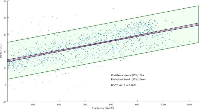
Finally, the prediction and confidence intervals were calculated to ensure the statistical significance of the linear regressions.
Confidence intervals consist of a range of values that act as good estimates of the unknown population parameter. With this method, for a pre-determined confidence level, a whole interval of acceptable values for the parameter is given instead of a single value.
The confidence interval is based on the observations from a sample, hence differing with sample size. Smaller samples generate wider intervals, following an inverse square root relationship between confidence intervals and sample sizes.
The prediction and confidence intervals were computed using the following equations.
𝐶𝑜𝑛𝑓𝑖𝑑𝑒𝑛𝑐𝑒𝐼𝑛𝑡𝑒𝑟𝑣𝑎𝑙: 𝑦1± 𝑡 × 𝑆𝐸 × √ 1 𝑙𝑒𝑛𝑔𝑡ℎ(𝑥)+
(𝑥1−𝑚𝑒𝑎𝑛(𝑥1))2
𝑠𝑢𝑚(𝑥−𝑚𝑒𝑎𝑛(𝑥))2 (4.2)
𝑃𝑟𝑒𝑑𝑖𝑐𝑡𝑖𝑜𝑛𝐼𝑛𝑡𝑒𝑟𝑣𝑎𝑙: 𝑦1± 𝑡 × 𝑆𝐸 × √1 + 1 𝑙𝑒𝑛𝑔𝑡ℎ(𝑥)+
(𝑥1−𝑚𝑒𝑎𝑛(𝑥1))2
𝑠𝑢𝑚(𝑥−𝑚𝑒𝑎𝑛(𝑥))2 (4.3)
The 𝑦1 represents the slope of the linear regression, to which the prediction and confidence intervals
will be added. The 𝑡 denotes the coefficient correspondent to the confidence level, according to the student’s 𝑡 distribution. Finally, SE stands for standard error, while the rest of the values are calculated. The confidence level was set at 95%, a level deemed adequate for our analysis. This level indicates that there’s a 95% chance that any point of the linear regression is within the calculated confidence interval. Conversely, there’s also a 95% percent chance that any individual sample point lies within the prediction interval.
In the image below are represented both the confidence and the prediction intervals for the linear regression of the Sharp module. The confidence interval of the linear regression is given by the blue lines, which are closing in on both sides of the linear regression marked in red.
Whereas the prediction bands are clearly defined, encompassing a larger area, the confidence intervals are almost undistinguishable from the regression line.
The narrowness of the confidence interval is a product of the large sample size, drawing on over one and a half thousand points to estimate the intervals.
Following the NOCT determination procedures, the value of NOCT is obtained by adjusting the difference between the module and ambient temperatures at 800 W/m2 to 20 ºC. As such, the uncertainty of this value will be given by the confidence values at this point.
For the Sharp solar panel, with a 95% confidence level, this resulted on a nominal operating cell temperature of 46 ± 0.2851 ºC.
This process was repeated for the other modules, ensuring the statistical relevance of this method.
Once again, the NOCT stayed within a very reasonable interval range, straying less than once percent of its estimated value. The largest confidence interval was found on the Panasonic solar module, whose data sample registered the most dispersion among the panels.
With a sample size of less than half of the other modules, the Panasonic solar panel displayed the largest confidence interval. This was due to the increased dispersion of the data, as hinted by the prediction bands, as well as the reduced sample size.
Nevertheless, its confidence interval remained extremely narrow, well within one percent of the parameter’s value.
Despite the small uncertainties in the NOCT calculation, inaccuracies of about ± 3 ºC in the NOCT value do not introduce excessive errors (about ± 1.5%) on the yearly performance estimations, as temperature has a second order influence on module energy output.
Having calculated the NOCT’s, it was now possible to determine the module’s temperature in function of the irradiance and ambient temperature. The modules’ temperature estimates were now available for the entire duration of the study without any gaps.
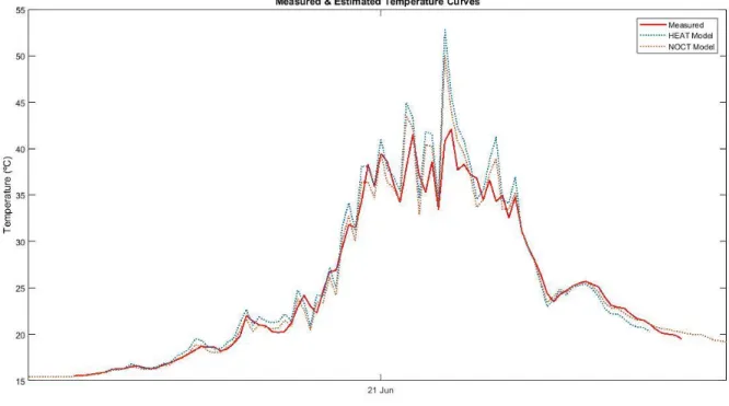
Then, in order to determine how accurately these new temperature curves described the real ones, the average mean absolute error was calculated. This indicator measures the average magnitude of the errors in our set of predictions, regardless of their direction.
This was done by comparing the measured and the estimated temperature curves, averaging the difference between them over the intervals where they had valid records.
The formula presented below was used in this process.
𝐸𝑟𝑟𝑜𝑟 (º𝐶) =∑𝑛𝑖=1| 𝑇𝑟𝑒𝑎𝑙(𝑖)−𝑇𝐸𝑠𝑡𝑖𝑚𝑎𝑡𝑒(𝑖) |
𝑛 (4.4)
This formula measures the average distance between these two curves at every single point of our valid domain. The valid domain encompasses all the intervals where the data points were different than zero. For the Sharp solar module, the mean error was of 3.24 ºC, giving us a very precise estimate of the module’s temperature during our study.
This error is close to the minimum possible obtainable error using equation (4.1), as we’ll see ahead, which means that it’s not possible to get a much more precise temperature estimate using this method. The NOCT obtained experimentally was 46.15 ºC for the Sharp solar module, which was used to draw the temperature curve. This curve is an accurate representation of the module’s thermal behavior; however, another method was employed in order to draw the temperature curves that best matched the real measured data.
These new curves were calculated through an iterative process of altering the NOCT, estimating the module’s temperature with equation (4.1), and comparing it to the real measured temperature curve by calculating the error following the same procedure as before.
The best curve fit resultant from this process, nicknamed the ideal temperature, was then the curve that minimized the error, thus best adapting to the real temperature data.
This method yielded the best results, with an average error of 3.23 ºC for the Sharp module. For this reason, the so-called ideal temperatures obtained from this method were prioritized.
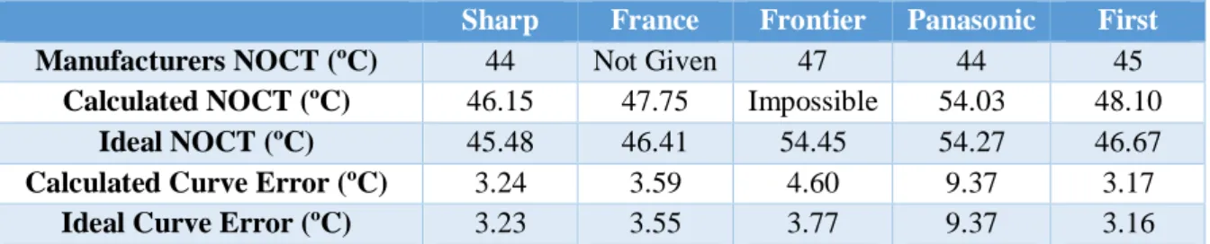
The table below summarizes some of the results for the panels studied:
Sharp France Frontier Panasonic First
Manufacturers NOCT (ºC) 44 Not Given 47 44 45
Calculated NOCT (ºC) 46.15 47.75 Impossible 54.03 48.10
Ideal NOCT (ºC) 45.48 46.41 54.45 54.27 46.67
Calculated Curve Error (ºC) 3.24 3.59 4.60 9.37 3.17
Ideal Curve Error (ºC) 3.23 3.55 3.77 9.37 3.16
Table 1: NOCT model results. Calculated and ideal NOCT values and their respective temperature curve errors.
There are three types of NOCT values referenced in this table, each obtained through a different method. The first one is the NOCT provided by the manufacturer in the datasheets. This value is often inadequate for temperature estimations, since in real operating conditions, different factors such as soiling can affect the nominal operating cell temperature. With this in mind, this value remained unused but was still referenced in the table, so as to allow a comparison between NOCT’s obtained through different methods.
The two other NOCT values were used to estimate and draw the module temperature curves, and are a product of two different methodologies.
The calculated NOCT was obtained by filtering the data and applying a linear regression, following the NOCT determination procedures designated in the IEC 61216 and IEC 61646. The ideal NOCT, however, was calculated through an iterative process of error minimization between the ideal and the measured temperatures. Having tested different NOCT’s over a reasonable interval range, the ideal NOCT was found to be the one that minimized the error, and thus whose resulting temperature curve best defined the real measured thermal behavior of the panels.
Finally on this table, are the calculated and ideal temperature errors. These correspond to the average errors between the real measured temperature points and the ones obtained through each procedure, measuring the success of each method.
While the calculated average error characterizes the average deviation between the measured and the calculated curves, the ideal average error denotes the error between the real measurements and the best possible temperature estimates using the IEC formula (4.1).
It’s worth noting that there weren’t sufficient reliable temperature records on the Solar Frontier module. As such, instead of calculating its NOCT through a linear regression, the manufacturers NOCT was used to draw the temperature curves for this panel.
In all cases, the ideal and calculated NOCT’s were always in close agreement, which suggests that the experimental method for the NOCT calculation is accurate, and that the temperature curves are near the best possible temperature estimates using the IEC NOCT determining procedures.
This precision is illustrated below in figure 4, for the France Watts solar module, where all three temperatures were plotted against each other.
As evidenced by the graph, there’s a very strong correlation between the real and estimated temperatures, which allows us to have continuous records of every module’s temperature during the entire duration of this study.
The cell temperature is essentially dependent on two main factors: Irradiance and air temperature. The air temperature heats the panel through conduction and convection, and conditions the minimum temperature the solar modules can achieve.
If it wasn’t for the irradiance, the solar modules’ temperature would follow the air temperature, with a certain thermal lag, depending on the insulating characteristics and thermal inertia of the panels. As such, the ambient temperature strongly affects the passive cooling of the PV panel, leading to an efficiency increase.
Solar irradiance, on the other hand, heats the panels through radiation, and the amount of heat transferred is proportional to the intensity of the irradiance.
Although there are several ways to minimize the heating effect caused by the Sun’s radiation, such as special coatings and better air circulation around the panel, there aren’t many solutions to counter the effects of air temperature.
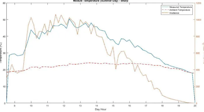
In order to better illustrate this relation, the Sharp panel’s real measured temperature was plotted over a day with a narrow ambient temperature variation range, thus allowing for a better visualization of the irradiance module temperature dependency.
The graph below shows the influence of these two parameters for the Sharp branded solar module during a typical summer day.
As we can observe, the module temperatures are strongly conditioned by the irradiance. This is particularly visible during this specific day due to the low range of the ambient temperatures.
Finally, in order to get a sense of how subtly the ambient temperature influences the module’s temperature, the same graph was plotted over the day of lowest irradiance.
Despite the record low irradiance values, it’s clear that the panel’s temperature is strongly influenced by the irradiance, whilst being baselined by the ambient temperature.
4.1.2. HEAT Thermal Model
Since temperature is a key parameter ruling the conversion efficiency, it was deemed important to try to further increase the accuracy of the temperature estimates. This would allow for a better correction of the efficiency values to STC conditions, leading to a more precise estimation of the soiling losses. The module temperature is dependent upon several factors, making it extremely difficult to obtain an accurate estimate. Simple estimates tend to rely on a few key parameters, such as ambient temperature, irradiance and NOCT. In order to increase the precision of this estimate, it’s necessary to increase quality of the model, taking into account the maximum number of relevant parameters, approaching the model to reality.
The HEAT model, as its name suggests, was based on the precise modelling of a panel’s energy fluxes. As such, the temperature of the panels will be estimated using a heat balance model, assuming the conservation of energy as follows:
𝐸𝑛𝑒𝑟𝑔𝑦𝐼𝑛𝑝𝑢𝑡 = 𝐸𝑛𝑒𝑟𝑔𝑦𝑂𝑢𝑡𝑝𝑢𝑡 (4.5)
This isn’t necessarily true at every single moment, as it’s this very imbalance of input and output energy that causes temperature to change, allowing for the estimation of the panels’ temperature.
The energy balance equation for our solar panel can be best described by the equation below:
𝑅𝑎𝑑𝑖𝑎𝑡𝑖𝑣𝑒𝐼𝑛𝑝𝑢𝑡= 𝑅𝑎𝑑𝑖𝑎𝑡𝑖𝑣𝑒𝑂𝑢𝑡𝑝𝑢𝑡+ 𝐶𝑜𝑛𝑣𝑒𝑐𝑡𝑖𝑣𝑒𝑂𝑢𝑡𝑝𝑢𝑡+ 𝐸𝑙𝑒𝑐𝑡𝑟𝑖𝑐𝑂𝑢𝑡𝑝𝑢𝑡 (4.6)
This simplified equation characterizes the heat balance of the solar module. The more accurate this model is, the more precise the temperature estimates will be. As evidenced by the equation, there is no mass transfer in our panel, making it a closed system.
In this equation, the radiative input corresponds to the total incident solar radiation on the panel. The radiative, convective and electric output correspond to the net energy transferred to or from the panel through those mechanisms.
These parameters were named outputs because they generally represent energy losses. However, these can be negative at times, when the ground radiation or air temperature heats the panels. Due to their relatively small contribution, the conduction losses were neglected in order to simplify the model. The first step on the construction of this model was the calculation of the radiative input on the solar panel. For this, the direct, diffuse, and reflected radiation were separated, giving a more detailed estimate of the incident radiation.
The incoming radiation was calculated with the following equation:
|--Direct--| |---Diffuse---| |---Reflected---|
𝑅𝑎𝑑𝑖𝑎𝑡𝑖𝑣𝑒𝐼𝑛𝑝𝑢𝑡= 𝐵𝑁𝐼× 𝐶𝑂+ 𝐷 × 𝐶𝑠× 𝐶𝐷+ 𝐺 × 𝑅𝐺× (1 − 𝐶𝑆) × 𝐶𝐷 (4.7)
BNI: Direct Irradiance (W/m2), CO: Average Transmissivity of the Glass for the Panel Inclination
D: Diffuse Irradiance (W/m2), C
S: Fraction of the Maximum Absorbable Diffuse Radiation
CD: Transmissivity Coefficient, G: Global Irradiance (W/m2)
RG: Average Reflective Index of the Surrounding Ground Floor
The transmissivity of the glass for direct radiation was fixed 0.67, which was the value previously calculated by integrating the transmissivities of the whole hemisphere. The transmissivity of the glass for diffuse radiation, on the other hand, is uniform and fixed at 0.8.
Finally, the average reflective index of the surrounding ground floor was fixed at 0.15, and the maximum absorbable fraction for diffuse and reflected radiation were calculated through the following formula:
𝐹𝑟𝑎𝑐𝑡𝑖𝑜𝑛𝐷𝑖𝑓𝑓𝑢𝑠𝑒 =
cos(𝑆𝑙𝑜𝑝𝑒)+1
2 [3.8]
It’s worth noting that, in the case of the reflected radiation, the opposite was true, and the maximum absorbable fraction was given by:
𝐹𝑟𝑎𝑐𝑡𝑖𝑜𝑛𝑅𝑒𝑓𝑙𝑒𝑐𝑡𝑒𝑑 = 1 −
cos(𝑆𝑙𝑜𝑝𝑒)+1
2 [3.9]
The image below details the panel’s estimated radiative input over two typical days, detailing the contribution of the different types of radiation to the total as well.
The radiative heat exchange between the panel and its surroundings was calculated according to the equation below.
|Emission| |Absorption|
𝑅𝑎𝑑𝑖𝑎𝑡𝑖𝑣𝑒𝑂𝑢𝑡𝑝𝑢𝑡 = 𝜀 × 𝛿 × [ 2𝑇𝑚4− (𝑇𝑠4− 𝑇𝑔4) ] [3.10]
ε: Emissivity of the Panel , δ: Stephan Boltzmann Constant (J/m2
K4)
A basic temperature estimate was needed for the calibration of the model, and for this task the NOCT model was used.
For simplification purposes, it was assumed that the emissivity did not depend on wavelength, emission angle or temperature, and it was fixed at 0.8, using the so called “Grey Body” approximation.
The ground and sky were extrapolated from the values of the Upwelling and Downwelling longwave horizontal irradiance, using the formulas below.
𝑇𝑔= ( 𝑈𝑝𝑤𝑒𝑙𝑙𝑖𝑛𝑔𝐿𝑜𝑛𝑔𝑤𝑎𝑣𝑒 δ ) 1 4 (4.11) 𝑇𝑠= ( 𝐷𝑜𝑤𝑛𝑤𝑒𝑙𝑙𝑖𝑛𝑔𝐿𝑜𝑛𝑔𝑤𝑎𝑣𝑒 δ ) 1 4 (4.12)
The convective balance of the module was calculated according to the formula below.
|Natural| |---Wind---| |Temperature|
𝐶𝑜𝑛𝑣𝑒𝑐𝑡𝑖𝑣𝑒𝑂𝑢𝑡𝑝𝑢𝑡= [ ℎ1+ (ℎ2× 𝑊𝑆𝐶𝑊𝑆) ] × (𝑇𝑚− 𝑇𝐴𝑖𝑟) (4.13)
h1: Convective Coefficient (W/m2K) , h2: Convective Coefficient (W/m2K)
WS: Wind Speed (m/s) , CWS: Coefficient of Convection dependency on Wind Speed Tm: Module Temperature (ºC) , TAir: Air Temperature (ºC)
As this image suggests, the convective losses are proportional to the temperature difference
between the panel and the ambient air. Wind speed is also represented, allowing for a more
complete modelling of the panel’s thermal behavior.
Finally, the electric output of the panel was calculated with the following formula:
|Efficiency| |---Correction---|
𝐸𝑙𝑒𝑐𝑡𝑟𝑖𝑐𝑂𝑢𝑡𝑝𝑢𝑡= 𝐴 × 𝐺 × Ƞ𝑆𝑇𝐶× [ 1 + 𝛽 × (𝑇𝑚− 25) ] × 𝐹 [3.14]
A: Solar Panel Area (m2) , G: Radiative Input (W/m2) , Ƞ
STC: Module Efficiency at STC (%)
β: Power Correction Coefficient (%/ºC) ,Tm: Module Temperature (ºC) ,
F: Electric Output Adjustment Factor