CERN-PH-EP/2013-148 2014/01/03
CMS-SUS-13-011
Search for top-squark pair production in the single-lepton
final state in pp collisions at
√
s
=
8 TeV
The CMS Collaboration
∗Abstract
This paper presents a search for the pair production of top squarks in events with a single isolated electron or muon, jets, large missing transverse momentum, and large transverse mass. The data sample corresponds to an integrated luminosity of 19.5 fb−1 of pp collisions collected in 2012 by the CMS experiment at the LHC at a center-of-mass energy of√s=8 TeV. No significant excess in data is observed above the expectation from standard model processes. The results are interpreted in the context of supersymmetric models with pair production of top squarks that decay either to a top quark and a neutralino or to a bottom quark and a chargino. For small mass values of the lightest supersymmetric particle, top-squark mass values up to around 650 GeV are excluded.
Published in the European Physical Journal C as doi:10.1140/epjc/s10052-013-2677-2.
c
2014 CERN for the benefit of the CMS Collaboration. CC-BY-3.0 license
∗See Appendix C for the list of collaboration members
1
Introduction
The standard model (SM) has been extremely successful at describing particle physics phenom-ena. However, it suffers from such shortcomings as the hierarchy problem, where fine-tuned cancellations of large quantum corrections are required in order for the Higgs boson to have a mass at the electroweak symmetry breaking scale of order 100 GeV [1–6]. Supersymmetry (SUSY) is a popular extension of the SM that postulates the existence of a superpartner for ev-ery SM particle, with the same quantum numbers but differing by one half-unit of spin. SUSY potentially provides a “natural”, i.e., not fine-tuned, solution to the hierarchy problem through the cancellations of the quadratic divergences of the top-quark and top-squark loops. In addi-tion, it provides a connection to cosmology, with the lightest supersymmetric particle (LSP), if neutral and stable, serving as a dark matter candidate in R-parity conserving SUSY models. This paper describes a search for the pair production of top squarks using the full dataset col-lected at√s=8 TeV by the Compact Muon Solenoid (CMS) experiment [7] at the Large Hadron Collider (LHC) during 2012, corresponding to an integrated luminosity of 19.5 fb−1. This search is motivated by the consideration that relatively light top squarks, with masses below around 1 TeV, are necessary if SUSY is to be the natural solution to the hierarchy problem [8–12]. These constraints are especially relevant given the recent discovery of a particle that closely resembles a Higgs boson, with a mass of∼125 GeV [13–15]. Searches for top-squark pair production have also been performed by the ATLAS Collaboration at the LHC in several final states [16–20], and by the CDF [21] and D0 [22] Collaborations at the Tevatron.
The search presented here focuses on two decay modes of the top squark (et): et → tχe01 and et→bχe
+. These modes are expected to have large branching fractions if kinematically allowed. Here t and b are the top and bottom quarks, and the neutralinos (χe
0) and charginos ( e
χ±) are
the mass eigenstates formed by the linear combination of the gauginos and higgsinos, which are the fermionic superpartners of the gauge and Higgs bosons, respectively. The charginos are unstable and may subsequently decay into neutralinos and W bosons, leading to the following processes of interest: pp → etet∗ → ttχe 0 1χe 0 1 → bbW+W−χe 0 1χe 0 1 and pp → etet∗ → bbχe + 1χe − 1 → bbW+W−χe 0 1χe 0
1, as displayed in Fig. 1. The lightest neutralinoχe 0
1is considered to be the stable LSP, which escapes without detection.
The analysis is based on events where one of the W bosons decays leptonically and the other hadronically. This results in one isolated lepton and four jets, two of which originate from b quarks. The two neutralinos and the neutrino from the W decay can result in large missing transverse momentum (Emiss
T ). P1 P2 ˜ t⇤ ˜ t ¯ t t ¯b W ˜0 1 ˜0 1 W+ b 3 P1 P2 ˜ t∗ ˜ t ˜ χ− W− ˜ χ+ W+ ¯b ˜ χ0 1 ˜ χ0 1 b
Figure 1: Diagram for top-squark pair production for (a) theet →tχe 0
1→bWχe 0
1decay mode and (b) theet→bχe
+→bW e
χ01decay mode.
2 3 Signal and background Monte Carlo simulation
where one top quark decays hadronically and the other leptonically, and from events with a W boson produced in association with jets (W+jets). These backgrounds, like the sig-nal, contain a single leptonically decaying W boson. The transverse mass, defined as MT ≡
√
2EmissT p`T(1−cos(∆φ)), where p`T is the transverse momentum of the lepton and ∆φ is the difference in azimuthal angles between the lepton and EmissT directions, has a kinematic end-point MT < MW for these backgrounds, where MW is the W boson mass. For signal events, the presence of LSPs in the final state allows MTto exceed MW. Hence we search for an excess of events with large MT. The dominant background with large MT arises from the “dilepton tt ” channel, i.e., tt events where both W bosons decay leptonically but with one of the leptons not identified. In these events the presence of two neutrinos can lead to large values of Emiss
T and MT.
2
The CMS detector
The central feature of the CMS apparatus is a superconducting solenoid, 13 m in length and 6 m in diameter, which provides an axial magnetic field of 3.8 T. Within the field volume are several particle detection systems. Charged-particle trajectories are measured with silicon pixel and strip trackers, covering 0 ≤ φ < 2π in azimuth and |η| < 2.5 in pseudorapidity, where η ≡ −ln[tan(θ/2)]and θ is the polar angle of the trajectory of the particle with respect to the
counterclockwise proton beam direction. A lead-tungstate crystal electromagnetic calorimeter and a brass/scintillator hadron calorimeter surround the tracking volume, providing energy measurements of electrons, photons, and hadronic jets. Muons are identified and measured in gas-ionization detectors embedded in the steel flux return yoke of the solenoid. The CMS detector is nearly hermetic, allowing momentum balance measurements in the plane transverse to the beam direction. A two-tier trigger system selects pp collision events of interest for use in physics analyses. A more detailed description of the CMS detector can be found elsewhere [7].
3
Signal and background Monte Carlo simulation
Simulated samples of SM processes are generated using the POWHEG [23], MC@NLO[24, 25], and MADGRAPH5.1.3.30 [26] Monte Carlo (MC) event generator programs with the CT10 [27]
(POWHEG), CTEQ6M [28] (MC@NLO), and CTEQ6L1 [28] (MADGRAPH) parton distribution
functions. The reference sample for tt events is generated with POWHEG, while the MAD
-GRAPHand MC@NLOgenerators are used for crosschecks and validations. All SM processes
are normalized to cross section calculations valid to next-to-next-to-leading order (NNLO) [29] or approximate NNLO [30] when available, and otherwise to next-to-leading order (NLO) [24, 25, 31–34].
For the signal events, the production of top-squark pairs is generated with MADGRAPH, in-cluding up to two additional partons at the matrix element level. The decays of the top squarks are generated with PYTHIA[35] assuming 100% branching fraction for eitheret → tχe
0
1 oret → bχe
+. A grid of signal events is generated as a function of the top-squark and neutralino masses in 25 GeV steps. We also consider scenarios with off-shell top quarks (foret→tχe
0 1) and off-shell W bosons (foret→bχe +followed by e χ+1 →W+χe 0 1). For theet→bχe
+decay mode, the chargino mass is specified by a third parameter x defined as m
e
χ1± = x·met+ (1−x) ·mχe
0
1. We consider three mass spectra, namely x = 0.25, 0.50, and 0.75. The lowest top squark mass that we con-sider is met= 100 GeV foret →tχe
0
1, and met= 200 (225, 150) GeV foret →bχe
+with x =0.25 (0.50, 0.75).
The polarizations of the final- and intermediate-state particles (top quarks in theet → tχe 0 1 sce-nario, and charginos and W bosons in theet → bχe
+case) are model dependent and are non-trivial functions of the top-squark, chargino, and neutralino mixing matrices [36, 37]. The SUSY MC events are generated without polarization. The effect of this choice on the final result is dis-cussed in Section 9. Expected signal event rates are normalized to cross sections calculated at NLO in the strong coupling constant, including the resummation of soft gluon emission at next-to-leading-logarithmic accuracy (NLO+NLL) [38–43].
For both signal and background events, multiple proton-proton interactions in the same or nearby bunch crossings (pileup) are simulated usingPYTHIA and superimposed on the hard collision. The simulation of the detector response to SUSY signal events is performed using the CMS fast simulation package [44], whereas almost all SM samples are simulated using a GEANT4-based [45] model of the CMS detector. The exceptions are the MADGRAPHtt samples used to study the sensitivity of estimated backgrounds to the details of the generator settings; these samples are processed with the fast simulation. The two simulation methods provide consistent results for the acceptances of processes of interest to this analysis. The simulated events are reconstructed and analyzed with the same software used to process the data.
4
Event selection
4.1 Object definition and event preselection
The data used for this search were collected using high transverse momentum (pT), isolated, single-electron and single-muon triggers with pTthresholds of 27 and 24 GeV, respectively. The electron (muon) trigger efficiency, as measured with a sample of Z→ ``events, varies between 85% and 97% (80% and 95%), depending on the η and pT of the leptons. Data collected with high-pTdouble-lepton triggers (ee, eµ, or µµ, with pT thresholds of 17 GeV for one lepton and 8 GeV for the other) are used for studies of dilepton control regions.
Events are required to have an electron (muon) with pT > 30(25)GeV. Electrons are required to lie in the barrel region of the electromagnetic calorimeter (|η| < 1.4442), while muons are
considered up to |η| = 2.1. Electron candidates are reconstructed starting from a cluster of
energy deposits in the electromagnetic calorimeter. The cluster is then matched to a recon-structed track. The electron selection is based on the shower shape, track-cluster matching, and consistency between the cluster energy and the track momentum [46]. Muon candidates are reconstructed by performing a global fit that requires consistent hit patterns in the tracker and the muon system [47].
The particle flow (PF) method [48] is used to reconstruct final-state particles. Leptons are re-quired to be isolated from other activity in the event. A measure of lepton isolation is the scalar sum (psumT ) of the pT of all PF particles, excluding the lepton itself, within a cone of radius ∆R ≡ √(∆η)2+ (∆φ)2 = 0.3, where∆η (∆φ) is the difference in η (φ) between the lepton and the PF particle at the primary interaction vertex. The average contribution of particles from pileup interactions is estimated and subtracted from the psumT quantity. The isolation require-ment is psumT < min(5 GeV, 0.15·p`T). Typical lepton identification and isolation efficiencies, measured in samples of Z → ``events, are 84% for electrons and 91% for muons, with varia-tions at the level of a few percent depending on pTand η.
To reduce the background from tt events in which both W bosons decay leptonically (denoted as tt → `` in the following), events are rejected if they contain evidence for an additional lepton. Specifically, we reject events with a second isolated lepton of pT > 5 GeV, identified
4 4 Event selection
with requirements that are considerably looser than for the primary lepton. We also reject events with an isolated track of pT > 10 GeV with opposite sign with respect to the primary lepton, as well as events with a jet of pT > 20 GeV consistent with the hadronic decay of a τ lepton [49]. The isolation algorithm used at this stage differs slightly from the one used in the selection of primary leptons: the cone has radius ∆R = 0.4, the psumT variable is constructed using charged PF particles only, and the isolation requirement is psumT < α·pT, where pT is the
transverse momentum of the track (lepton) and α=0.1(0.2), for tracks (leptons).
The PF particles are clustered to form jets using the anti-kT clustering algorithm [50] with a distance parameter of 0.5, as implemented in the FASTJETpackage [51, 52]. The contribution to the jet energy from pileup is estimated on an event-by-event basis using the jet area method described in Ref. [53], and is subtracted from the overall jet pT. Jets from pileup interactions are suppressed using a multivariate discriminant based on the multiplicity of objects clustered in the jet, the topology of the jet shape, and the impact parameters of the charged tracks with respect to the primary interaction vertex. The jets must be separated from the lepton by∆R>
0.4 in order to resolve overlaps.
Selected events are required to contain at least four jets with pT > 30 GeV and |η| < 2.4. At
least one of these jets must be consistent with containing the decay of a heavy-flavor hadron, as identified using the medium operating point of the combined secondary vertex bottom-quark (b-bottom-quark) tagging algorithm (CSVM) [54]. We refer to such jets as “b-tagged jets”. The efficiency of this algorithm for bottom-quark jets in the pT range 30–400 GeV varies between approximately 60 and 75% for|η| <2.4. The nominal misidentification rate for light-quark or
gluon jets is 1% [54].
The missing transverse momentum is defined as the magnitude of the vector sum of the trans-verse momenta of all PF particles over the full calorimeter coverage (|η| <5). The EmissT vector
is the negative of that same vector sum. The calibrations that are applied to the energy measure-ments of jets are propagated consistently as a correction to the ETmissobtained from PF particles. We require EmissT >100 GeV.
To summarize, events are required to contain one isolated lepton (e or µ), no additional iso-lated track or hadronic τ-lepton candidate, at least four jets with at least one b-tagged jet, and ETmiss > 100 GeV; this is referred to below as the “event preselection”. Signal regions are de-fined demanding MT>120 GeV. This requirement provides large suppression of the SM back-grounds while retaining high signal efficiency. Requirements on several kinematic quantities or on the output of boosted decision tree (BDT) multivariate discriminants are also used to define the signal regions, as described below.
4.2 Kinematic quantities
To reduce the dominant tt→ ``background, we make use of the quantity MT2W, defined as the minimum “mother” particle mass compatible with all the transverse momenta and mass-shell constraints [55]. This variable is a variant of the MT2observable [56–58], and is designed specif-ically to suppress the tt→ ``background with one undetected lepton in the top squark search. By construction, for the dilepton tt background without mismeasurement effects, MW
T2 has an endpoint at the top-quark mass. The MW
T2 calculation relies on the correct identification of the b-quark jets and the correct pairing of the b-quark jets with the leptons. The MWT2value in the event is defined as the minimum of the MWT2 values calculated from all possible combinations of b-quark jets and the lepton. For events with only one b-tagged jet, the combinations are performed using each of the three remaining highest pTjets as the possible second b-quark jet.
In theet → tχe 0
1 search, the dilepton tt background is suppressed by requiring that three of the jets in the event be consistent with the t → bW → bq ¯q decay chain. For each triplet of jets in the event we construct a hadronic top χ2as:
χ2= (Mj1j2j3−Mtop) 2 σ2j 1j2j3 +(Mj1j2 −MW) 2 σj2 1j2 . (1)
Here Mj1j2j3 is the mass of the three-jet system, Mj1j2 is the mass of two of the jets posited to originate from W boson decay, and σj1j2j3 and σj1j2 are the uncertainties on these masses calculated from the jet energy resolutions [59]. The three-jet mass Mj1j2j3 is computed after requiring Mj1j2 = MW using a constrained kinematic fit, while Mj1j2 in Eqn. 1 is the two-jet mass before the fit. Finally, Mtop = 173.5 GeV (MW = 80.4 GeV) is the mass of the top quark (W boson) [60]. The three jets are required to have pT >30 GeV and|η| <2.4 and to be among
the six leading selected jets. The jet assignments are made consistently with the b-tagging information, i.e., j3must be b-tagged if there are at least two b-tagged jets and j1and j2cannot be b-tagged unless there are at least three b-tagged jets in the event. The minimum hadronic top χ2 amongst all possible jet combinations is used as a discriminant on an event-by-event basis.
Two topological variables are used in the selection of signal candidates. The first is the mini-mum∆φ value between the EmissT vector and either of the two highest pTjets, referred to below as “min∆φ”. Background tt events tend to have high-pT top quarks, and thus objects in these events tend to be collinear in the transverse plane, resulting in smaller values of ∆φ than is typical for signal events. The second variable is HTratio, defined as the fraction of the total scalar sum of the jet transverse energies (HT) with pT > 30 GeV and|η| < 2.4 that lies in the same hemisphere as the EmissT vector. This quantity tends to be smaller for signal than for background events, because in signal events the visible particles recoil against the LSPs, resulting on aver-age in events with more energy in the opposite hemisphere to the EmissT .
In theet → bχe
+decay mode, the bottom quarks arise from the decay of the top squark, while in background events they originate from the decay of the top quark. As a result, in most of the signal parameter space the pT spectrum of the bottom quarks is harder for signal than for background events. Conversely, in theet → tχe
0
1 decay mode, if the top quark is off-shell, the pT spectrum of the bottom quarks is softer for signal than for the background. The pT value of the highest-pT b-tagged jet is therefore a useful discriminant. An additional, related, discriminating variable is the ∆R separation between this jet and the lepton. Finally, the pT spectrum of the lepton can be used to discriminate between on-shell and off-shell leptonic W decays, which occur in theet → bχe
+mode when the mass splitting between the chargino and the LSP is smaller than the W boson mass.
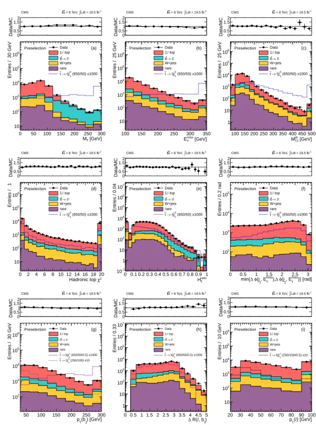
The distributions after the preselection of EmissT , MT, and the kinematic quantities described above, are shown in Fig. 2. These quantities are seen to be in agreement with the simulation of the SM background processes that will be discussed in more detail in Section 5.
4.3 Signal region definition
Two approaches are pursued to define the signal regions (SRs): a “cut-based” approach based on sequential selections on individual variables, and a BDT multivariate approach implemented via the TMVA package [61]. In both methods, we apply the preselection requirements of Sec-tion 4.1. The cut-based signal regions are defined by adding requirements on individual kine-matic variables. In contrast, the BDT combines the kinekine-matic variables into a single discrimi-nant, and the BDT SRs are defined by requirements on this discriminant. The BDT approach
6 4 Event selection [GeV] T M 0 50 100 150 200 250 300 Entries / 30 GeV 10 2 10 3 10 4 10 5 10 6 10 Data top l 1 ll → t t W+jets rare (650/50) x1000 0 1 χ∼ t → t ~ Preselection (a) -1 Ldt = 19.5 fb ∫ = 8 TeV, s CMS Data/MC0.50 1 1.5 2 [GeV] miss T E 100 150 200 250 300 350 Entries / 25 GeV 10 2 10 3 10 4 10 5 10 6 10 Data top l 1 ll → t t W+jets rare (650/50) x1000 0 1 χ∼ t → t ~ Preselection (b) -1 Ldt = 19.5 fb ∫ = 8 TeV, s CMS Data/MC0.50 1 1.5 2 [GeV] W T2 M 100 150 200 250 300 350 400 450 500 Entries / 25 GeV 1 10 2 10 3 10 4 10 5 10 6 10 Data top l 1 ll → t t W+jets rare (650/50) x1000 0 1 χ∼ t → t ~ Preselection (c) -1 Ldt = 19.5 fb ∫ = 8 TeV, s CMS Data/MC0.50 1 1.5 2 2 χ Hadronic top 0 2 4 6 8 10 12 14 16 18 20 Entries / 1 10 2 10 3 10 4 10 5 10 6 10 Data top l 1 ll → t t W+jets rare (650/50) x1000 0 1 χ∼ t → t ~ Preselection (d) -1 Ldt = 19.5 fb ∫ = 8 TeV, s CMS Data/MC0.50 1 1.5 2 ratio T H 0 0.1 0.2 0.3 0.4 0.5 0.6 0.7 0.8 0.9 1 Entries / 0.04 -1 10 1 10 2 10 3 10 4 10 5 10 6 10 7 10 Data top l 1 ll → t t W+jets rare (650/50) x1000 0 1 χ∼ t → t ~ Preselection (e) -1 Ldt = 19.5 fb ∫ = 8 TeV, s CMS Data/MC0.50 1 1.5 2 [rad] )} miss T , E 2 (j φ ∆ ), miss T , E 1 (j φ ∆ min{ 0 0.5 1 1.5 2 2.5 3 Entries / 0.2 rad 2 10 3 10 4 10 5 10 Data top l 1 ll → t t W+jets rare (650/50) x1000 0 1 χ∼ t → t ~ Preselection (f) -1 Ldt = 19.5 fb ∫ = 8 TeV, s CMS Data/MC0.50 1 1.5 2 ) [GeV] 1 (b T p 50 100 150 200 250 300 Entries / 30 GeV 2 10 3 10 4 10 5 10 6 10 Data top l 1 ll → t t W+jets rare (650/50/0.5) x1000 ± 1 χ∼ b → t ~ (250/100) x10 0 1 χ∼ t → t ~ Preselection (g) -1 Ldt = 19.5 fb ∫ = 8 TeV, s CMS Data/MC0.50 1 1.5 2 ) 1 , b l R( ∆ 0 0.5 1 1.5 2 2.5 3 3.5 4 4.5 5 Entries / 0.33 1 10 2 10 3 10 4 10 5 10 6 10 7 10 Data top l 1 ll → t t W+jets rare (650/50/0.5) x1000 ± 1 χ∼ b → t ~ Preselection (h) -1 Ldt = 19.5 fb ∫ = 8 TeV, s CMS Data/MC0.50 1 1.5 2 ) [GeV] l ( T p 20 30 40 50 60 70 80 90 100 Entries / 10 GeV 10 2 10 3 10 4 10 5 10 6 10 Data top l 1 ll → t t W+jets rare (250/150/0.5) x10 ± 1 χ∼ b → t ~ Preselection (i) -1 Ldt = 19.5 fb ∫ = 8 TeV, s CMS Data/MC 0 0.5 1 1.5 2
Figure 2: Comparison of data with MC simulation for the distributions of (a) MT, (b) EmissT , (c) MW
T2, (d) hadronic top χ2, (e) HTratio, (f) minimum ∆φ between the ETmiss vector and the two leading jets, (g) pT of the leading b-tagged jet, (h)∆R between the leading b-tagged jet and the lepton, and (i) lepton pT, after the preselection. For the plots (a)-(f), distributions for theet→tχe
0 1 model with met =650 GeV and m
e
χ01 =50 GeV, scaled by a factor of 1000, are overlayed. We also show distributions ofet→tχe
0
1with met =250 GeV and mχe 0
1 = 100 GeV for (g), scaled by 10, and ofet → bχe
+with m
et = 650 GeV, mχe 0
1 = 50 GeV, and x = 0.5 for (h) and (i), scaled by 1000, as well as of met = 250 GeV, m
e
χ01 = 150 GeV, and x = 0.5 for (i), scaled by 10. In all distributions the last bin contains the overflow.
improves the expected sensitivity of the search by up to 40% with respect to the cut-based ap-proach, at the cost of additional complexity. The primary result of our search is obtained with the BDT, while the cut-based analysis serves as a crosscheck. Table 1 lists the variables used in the training of the BDTs (Section 4.3.1) and summarizes the requirements for the cut-based SRs (Section 4.3.2).
Table 1: Summary of the variables used as inputs for the BDTs and of the kinematic require-ments in the cut-based analysis. All signal regions include the requirement MT >120 GeV. For theet→tχe
0
1BDT trained in the region where the top quark is off-shell, the hadronic top χ2is not included and the leading b-tagged jet pTis included. The lepton pTis used only in the training of theet→bχe
+BDT in the case where the W boson is off-shell.
et→teχ01 et→beχ
+
Cut-based Cut-based
Selection BDT Low∆M High∆M BDT Low∆M High∆M
ETmiss(GeV) yes >250, 300150, 200, >250, 300150, 200, yes >200, 250100, 150, >200, 250100, 150, MW
T2(GeV) yes >200 yes >200
min∆φ yes >0.8 >0.8 yes >0.8 >0.8
Hratio
T yes yes
Hadronic top χ2 (on-shell top) <5 <5
Leading b-tagged jet pT(GeV) (off-shell top) yes >100
∆R(`,leading b-tagged jet) yes
Lepton pT(GeV) (off shell W)
4.3.1 BDT signal regions
The BDTs are trained on samples of MC signal and background events satisfying the preselec-tion requirements and with MT > 120 GeV. The BDTs are trained with MADGRAPHsamples foret → tχe
0
1 and a mixture of MADGRAPH andPYTHIA samples foret → bχe
+. The choice of generators has little impact on the final result. The background MC sample contains all the expected SM processes.
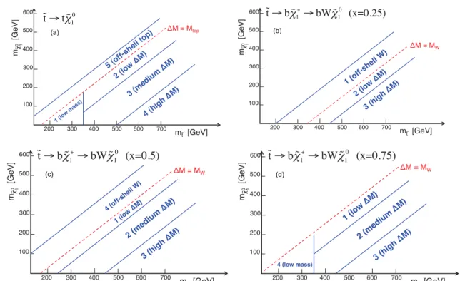
Separate BDTs are trained for theet→ tχe01andet →bχe+decay modes and for different regions of parameter space. In what follows we refer to the different BDTs as BDTn, where n is the region number defined in Fig. 3. In general, for a given BDT, the optimal requirement does not depend strongly on the point in parameter space within each region. Thus, for almost all regions a single BDT requirement is sufficient, and each such requirement defines a BDT signal region. The exceptions are BDT1 for theet→tχe
0
1signal model and BDT2 for theet→bχe
+signal model with parameter x =0.5; in these regions we choose two BDT operating points, referred to as “tight” and “loose”.
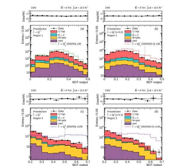
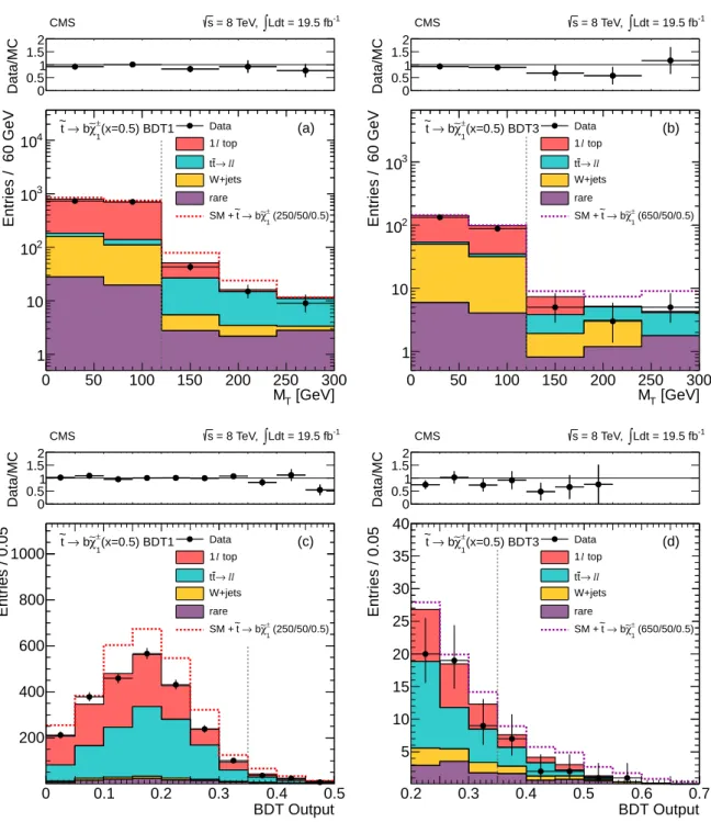
BDT distributions after the preselection are shown in Fig. 4 for four of the 16 BDTs (two tight and two loose BDTs). The data are in agreement with the MC simulation of SM processes.
4.3.2 Cut-based signal regions
For theet → tχe 0
1 model, two types of signal regions are distinguished: those targeting “small ∆M” and those targeting “large ∆M”, where ∆M ≡ met−m
e
χ0. Both categories include the requirement that the azimuthal angular difference between the two leading jets and the EmissT vector exceed 0.8 radians, in addition to the requirement that the value of the hadronic top
χ2 be less than 5. The MWT2 > 200 GeV requirement is applied only for the large ∆M signal
regions. Within each set, the SRs are distinguished by four successively tighter EmissT require-ments: Emiss
T >150, 200, 250, and 300 GeV. For theet →bχe
+model, the same approach is followed as for
et → tχe 0
1 by defining two sets of signal regions, one for small∆M and one for high ∆M, where ∆M here is the mass difference
8 5 Background estimation methodology 200 300 400 500 600 700 100 200 300 400 500 600 mt~ [GeV] M = Mtop t t 10 m [GeV]0 1 ~ 200 300 400 500 600 700 100 200 300 400 500 600 2 (low M) 3 (high M) mt~ [GeV] M = MW t b 1+ bW 1 0 (x=0.25) m [GeV]0 1 ~ 1 (off-shell W) 1 (low M) 200 300 400 500 600 700 100 200 300 400 500 600 2 (medium M) 3 (high M) mt~ [GeV] M = MW t b 1 + bW 1 0 (x=0.5) m [GeV]0 1 ~ 4 (off-shell W) 1 (low M) 200 300 400 500 600 700 100 200 300 400 500 600 2 (medium M) 3 (high M) 4 (low mass) mt~ [GeV] M = MW t b 1 + bW 1 0 (x=0.75) m [GeV]0 1 ~
Figure 3: The regions used to train the BDTs, in the m e
χ01 vs. met parameter space, for (a) the et →tχe
0
1scenario, and for (b) theet →bχe
+x = 0.25, (c) 0.5, and (d) 0.75 scenarios. The dashed lines correspond to ∆M ≡ m et−mχe 0 1 = Mtop foret → tχe 0 1, and∆M ≡ mχ+1 −mχe 0 1 = MW for et→bχe +.
between the chargino and the LSP. Just as in theet→tχe 0
1case, SRs are distinguished by increas-ingly tighter requirements on ETmiss. Since in the case ofet→bχe
+the signal has no top quark in its decay products, the requirement on the hadronic top χ2is not used. The large∆M selection includes the MT2Wrequirement, as well as the requirement that the leading b-tagged jet have pT larger than 100 GeV.
4.3.3 Signal regions summary
To summarize, this search uses two complementary approaches: one a cut-based approach and the other a BDT multivariate method. Correspondingly, there are two distinct sets of signal regions. In the BDT case, the SRs are defined by requirements on the BDT outputs. The BDT SRs provide the primary result, since the BDT method has better expected sensitivity. There are a total of 16 cut-based SRs (eight each for theet →tχe
0
1andet →bχe
+cases) and 18 BDT SRs (six for theet→tχe
0
1mode and 12 for theet →bχe
+mode). The expected number of background events in the SRs varies between approximately 4 and 1600 (see Section 8).
5
Background estimation methodology
The SM background is divided into four categories that are evaluated separately. The largest background contribution after full selection is tt production in which both W bosons decay leptonically (tt → ``), but one of the leptons is not identified. The second largest background consists of tt production in which one W boson decays leptonically and the other hadroni-cally (tt→ ` +jets), as well as single-top-quark production in the s- and t-channels: These are
BDT output 0 0.2 0.4 0.6 Entries / 0.05 10 2 10 3 10 4 10 5 10 6 10 7 10 Data1 l top ll → t t W+jets rare (250/50) x30 0 1 χ∼ t → t ~ Preselection 0 χ∼ t → t ~ Region 1 (a) -1 Ldt = 19.5 fb ∫ = 8 TeV, s CMS Data/MC 0 0.51 1.52 BDT output 0 0.1 0.2 0.3 0.4 0.5 Entries / 0.05 10 2 10 3 10 4 10 5 10 6 10 Data top l 1 ll → t t W+jets rare (250/50/0.5) x30 ± 1 χ∼ b → t ~ Preselection (x=0.5) ± χ∼ b → t ~ Region 1 (b) -1 Ldt = 19.5 fb ∫ = 8 TeV, s CMS Data/MC 0 0.51 1.52 BDT output 0.2 0.3 0.4 0.5 0.6 0.7 Entries / 0.05 1 10 2 10 3 10 4 10 Data top l 1 ll → t t W+jets rare (650/50) x100 0 1 χ∼ t → t ~ Preselection 0 χ∼ t → t ~ Region 4 (c) -1 Ldt = 19.5 fb ∫ = 8 TeV, s CMS Data/MC 0 0.51 1.52 BDT output 0.2 0.3 0.4 0.5 0.6 0.7 Entries / 0.05 1 10 2 10 3 10 4 10 Data top l 1 ll → t t W+jets rare (650/50/0.5) x100 ± 1 χ∼ b → t ~ Preselection (x=0.5) ± χ∼ b → t ~ Region 3 (d) -1 Ldt = 19.5 fb ∫ = 8 TeV, s CMS Data/MC 0 0.51 1.52
Figure 4: Comparison of data and MC simulation for sample BDT outputs. (a)et→tχe 0
1scenario in training region 1; (b)et→bχe
+scenario with x=0.5 in training region 1; (c)
et→tχe 0
1scenario in training region 4; (d)et → bχe
+ scenario with x = 0.5 in training region 3. Only the event preselection is applied, and in all cases the last bin contains the overflow. Events in the signal regions are further selected by requiring MT > 120 GeV and by applying BDT requirements as indicated by the vertical dashed lines. We also overlay expectations for possible signals with met = 250 GeV and m
e
χ01 = 50 GeV (panels (a) and (b)) and met = 650 GeV and mχe 0 1 = 50 GeV (panels (c) and (d)). For display purposes, these are scaled up by factors of 30 and 100 respectively.
collectively referred to as “single-lepton-top-quark” processes. The third largest background consists of a variety of SM processes with small cross sections, including tt events produced in association with a vector boson (ttW, ttZ, ttγ), processes with two (WW, WZ, ZZ) and three (WWW, WWZ, WZZ, ZZZ) electroweak vector bosons, and single-top-quark production in the tW-channel. These processes are collectively referred to as the “rare” processes. The fourth and final background contribution is from the production of W bosons with jets (W+jets). The multijet contribution to the background is negligible in the signal regions due to the require-ment of a high-pT isolated lepton, large MT, large EmissT , and a b-tagged jet. Here, “multijet” refers to events composed entirely of jets, without a lepton, W or Z boson, or top quark. Backgrounds are estimated from MC simulations, with small corrections (see below). The sim-ulation is validated in control regions (CRs) designed to enrich the data sample in specific
10 5 Background estimation methodology
sources of background while maintaining kinematic properties that are similar to those in the signal regions (see Section 6). In the CRs the kinematic variables used in the cut-based and BDT selections are examined to verify that they are properly modeled. A key distribution in each CR is that of MTafter the cut-based or BDT selection requirements, since MT >120 GeV is the final criterion that defines each signal region. The data/MC comparison of the number of events with MT > 120 GeV is then a direct test of the ability of the method to correctly predict the SM background in the signal regions.
The CR studies are designed to extract data/MC scale factors to be applied to the MC predic-tions for the background in the signal regions. We find that the only scale factor required is related to an underestimation of the MT tail for single-lepton-top-quark and W+jets events, as discussed in more detail in Section 6.
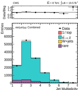
Jet Multiplicity 1 2 3 4 5 6 7 8 Entries 0 1000 2000 3000 4000 5000 6000 7000 Data top l 1 ll → t t W+jets rare Combined µ µ e/ µ ee/ -1 Ldt = 19.5 fb ∫ = 8 TeV, s CMS Data/Bkg 0.60.8 1 1.2 1.4
Figure 5: Comparison of the jet multiplicity distributions in data and MC simulation in the sample dominated by tt→ ``events.
The selection of signal events requires at least four hadronic jets. As mentioned above, the dominant background consists of tt → ``events with one unidentified lepton. These events satisfy the signal region selection only if there are two additional jets from initial- or final-state radiation (ISR/FSR) or if there is one such jet in conjunction with a second lepton identified as a jet (e.g., in the case of hadronic τ-lepton decays). To validate the modeling of ISR/FSR, a data control sample of tt → `` events is defined by requiring the presence of exactly two opposite-sign leptons (electrons or muons) in events satisfying dilepton triggers. To suppress the Z+jets background that is present in this control sample, same-flavor (ee or µµ) events with an invariant mass in the range 76< m``< 106 GeV are rejected, the presence of at least one b-tagged jet is required, and minimum requirements are imposed on EmissT . We then compare the distribution of the number of jets in data and MC simulation, as displayed in Fig. 5. The fraction of tt→ ``events with three or more jets is found to be in agreement with the expectation from the MC simulation within a 3% statistical uncertainty.
To minimize systematic uncertainties associated with the tt production cross section, integrated luminosity, lepton efficiency, and jet energy scale, the tt MC backgrounds at high MT are al-ways normalized to the number of events in data in the transverse-mass peak region, defined as 50 < MT < 80 GeV, after subtracting the contribution from rare backgrounds. We refer to this normalization factor as the “tail-to-peak ratio”. Background contributions from rare
processes are taken directly from the simulated samples. Their rates are normalized using the corresponding NLO cross sections.
6
Control region studies
Three CRs are used in this analysis. A sample dominated by tt → ``events is obtained by requiring the presence of two leptons (CR-2`). A sample dominated by a mixture of tt → ` +
jets and tt→ ``events is obtained by requiring the presence of a lepton and one isolated track or hadronic τ-lepton candidate (CR-`t). A sample dominated by W+jets events is obtained by vetoing events with b-tagged jets (CR-0b).
In all CRs, we apply the various SR selections and compare data and MC yields with MT > 120 GeV after normalizing the MTdistribution to the transverse-mass peak region as described in Section 5. In the case of CR-2`, the definition of MT is ambiguous because there are two identified leptons; we take the MT value constructed from the leading lepton and the EmissT vector.
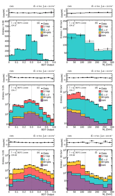
The BDT output distribution trained inet→tχe 0
1region 1 (BDT1) is shown in Fig. 6 for the three control regions. The MTdistribution after the BDT signal region requirement is also displayed (in the case of CR-0b this is corrected using the scale factor discussed below). Similar levels of agreement between data and MC simulation are found for the other SR-like selections.
For CR-2`and CR-`t, the number of data events with MT >120 GeV is consistent with the MC prediction. The level of agreement is used to assess a systematic uncertainty for the tt → ``
background prediction. The uncertainty ranges from 5% for the loosest signal regions to 70% for the tightest signal regions, reflecting the limited statistical precision of the control samples after applying the MT and BDT requirements. The fraction of events in CR-2`and CR-`t with MT >120 GeV that could be from stop pair production varies between approximately 1% and 20%, depending on the CR and the masses of the top squark and the LSP. This contribution is always much smaller than the statistical uncertainty on the data event counts.
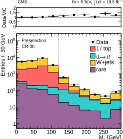
In the case of CR-0b, the transverse-mass distribution of events exhibits a small excess at high MT with respect to the MC prediction. This discrepancy, illustrated in Fig. 7 using the high-statistics samples of the preselection level, is attributed to imperfect modeling of the tails of the Emiss
T resolution in W+jets events. The data/MC agreement in the CR-0b MT tail can be restored by rescaling the W+jets contribution by a factor of 1.2±0.3, as seen for example in Fig. 6, bottom right. We find that this factor is insensitive to the details of the selection of the kinematic variables in Table 1 for the CR-0b event sample.
The observation that the simulation underestimates the MTtail in the W+jets sample suggests that a similar effect should exist in the single-lepton-top-quark background. However, the MT tail is more populated for the W+jets background than for the single-lepton-top-quark background, due to a significant contribution from very off-shell W bosons. This contribution is much less pronounced for the single-lepton-top-quark background because, ignoring the top-quark width, the lepton-neutrino mass M`νcannot exceed the difference between the top-and bottom-quark masses, M`ν < Mtop−Mb. This bound can be violated only if both the top quark and W boson from top quark decays are off-shell. For this reason the scale factor of 1.2±0.3 measured in W+jets events cannot be simply applied to the single-lepton-top-quark simulated sample. The scale factor is larger in the single-lepton-top-quark sample because the fraction of events that have MT > 120 GeV due to ETmissmismeasurement is larger than in the W+jets sample.
12 6 Control region studies BDT Output 0 0.1 0.2 0.3 0.4 0.5 0.6 Entries / 0.08 100 200 300 400 500 600 700 800 Data top l 1 ll → t t W+jets rare BDT1 Loose 0 1 χ∼ t → t ~ l CR-2 (a) -1 Ldt = 19.5 fb ∫ = 8 TeV, s CMS Data/MC 0.50 1 1.52 [GeV] T M 0 50 100 150 200 250 300 Entries / 60 GeV 50 100 150 200 250 Data top l 1 ll → t t W+jets rare BDT1 Loose 0 1 χ∼ t → t ~ l CR-2 (b) -1 Ldt = 19.5 fb ∫ = 8 TeV, s CMS Data/MC 0.50 1 1.52 BDT Output 0 0.1 0.2 0.3 0.4 0.5 0.6 Entries / 0.05 10 2 10 3 10 4 10 Data top l 1 ll → t t W+jets rare BDT1 Loose 0 1 χ∼ t → t ~ t l CR-(c) -1 Ldt = 19.5 fb ∫ = 8 TeV, s CMS Data/MC 0.50 1 1.52 [GeV] T M 0 50 100 150 200 250 300 Entries / 30 GeV 10 2 10 3 10 Data top l 1 ll → t t W+jets rare BDT1 Loose 0 1 χ∼ t → t ~ t l CR-(d) -1 Ldt = 19.5 fb ∫ = 8 TeV, s CMS Data/MC 0.50 1 1.52 BDT Output 0 0.1 0.2 0.3 0.4 0.5 0.6 Entries / 0.05 10 2 10 3 10 4 10 5 10 Data1 l top ll → t t W+jets rare BDT1 Loose 0 1 χ∼ t → t ~ CR-0b (e) -1 Ldt = 19.5 fb ∫ = 8 TeV, s CMS Data/MC 0 0.51 1.52 [GeV] T M 0 50 100 150 200 250 300 Entries / 30 GeV 1 10 2 10 3 10 4 10 5 10 Data top l 1 ll → t t W+jets rare BDT1 Loose 0 1 χ∼ t → t ~ CR-0b (f) -1 Ldt = 19.5 fb ∫ = 8 TeV, s CMS Data/MC 0 0.51 1.52
Figure 6: Comparison of data and MC simulation for the distributions of MTand BDT output for the control regions associated with the BDT trained in region 1 for theet→tχe
0
1scenario. The MT distributions are shown after the “BDT1 loose” requirement indicated by vertical dashed lines on the BDT output plots. (a)-(b): CR-2`; (c)-(d): CR-`t; (e)-(f): CR-0b. The vertical dashed lines in the MT plots correspond to the MT > 120 GeV selection requirement. For CR-0b, the scale factors are applied to the MC distribution in the MT tail. The last bin in all distributions contains the overflow.
[GeV] T M 0 50 100 150 200 250 300 Entries / 30 GeV 1 10 2 10 3 10 4 10 5 10 Data top l 1 ll → t t W+jets rare Preselection CR-0b -1 Ldt = 19.5 fb ∫ = 8 TeV, s CMS Data/MC 0 0.51 1.52
Figure 7: Comparison of data and MC simulation for the MTdistribution in the CR-0b control region, after the preselection. The MT tail is underestimated by the simulation. A scale factor derived from this control region is used to correct the predictions of the W+jets and single-lepton-top-quark backgrounds. The last bin of the distribution includes the overflow.
Following the arguments given above, a lower bound on the data tail-to-peak ratio for the single-lepton-top-quark sample (Rtop) can be obtained by scaling the MC value of Rtopby the W+jets scale factor (1.2±0.3). Conversely, an upper bound for Rtopis Rtop = RW+jets, where RW+jetsis the tail-to-peak ratio for W+jets in the data, i.e., its MC value scaled up by 1.2±0.3. This is an overestimate of the true value of Rtopbecause, as mentioned above, the MT tail is more populated for the W+jets sample than for the one-lepton-top sample. Since the true value of Rtop lies between these two extremes, we take the average of the upper and lower bounds. The resulting scale factor for Rtop with respect to its uncorrected MC result lies be-tween 1.5 and 2, depending on the signal region. The associated uncertainty includes the sta-tistical uncertainty in the data/MC scale factor from CR-0b, and half the difference between these upper and lower bounds.
7
Systematic uncertainties of the background prediction
All backgrounds except for the rare contribution are normalized to data in the MT-peak region, so the statistical uncertainties of the data and MC yields in the MT-peak region contribute to the uncertainty of the background predictions in the high-MT signal regions. This normalization is repeated after varying the W+jets background yield in the MT-peak region by ±50% to estimate the associated systematic uncertainty.
For the tt → ``background, the dominant uncertainty is assessed by comparing the data and MC yields in the high-MTregions of the CR-2`and CR-`t samples after applying the kinematic requirements for the corresponding signal region. This uncertainty varies between 5% and 70%. The uncertainty for the modeling of additional jets from radiation in tt → ``events results in a 3% uncertainty on the dilepton background. The uncertainty from the limited number of events in the tt→ ``MC sample also contributes, particularly in the tight signal regions. An additional uncertainty is associated with the efficiency to identify a second lepton (e, µ, or one-prong hadronic τ-lepton decay) as an isolated track. We verify that the simulation
re-14 8 Results
produces the efficiency of the isolated track requirement through studies of Z→ ``events in data, and we assign a systematic uncertainty of 6%. An uncertainty of 7%, based on studies of the efficiency for τ-lepton identification in data and simulation, is applied to events with a hadronic τ-lepton in the hadronic τ-lepton veto acceptance. We also verify the stability of the tt→ ``MC background prediction by comparing the results of the nominalPOWHEGsample with those obtained using MADGRAPH andMC@NLO, by varying the MADGRAPH scale pa-rameters for renormalization and factorization, as well as the scale for the matrix element and parton shower matching, up and down by a factor of two, and by varying the top-quark mass in the range 178.5 to 166.5 GeV. Since the resulting background predictions are consistent within the systematic uncertainties discussed above, we do not assess an additional uncertainty from the tt MC stability tests.
The uncertainty of the W+jets background prediction is dominated by the uncertainty from the tail-to-peak ratio, as determined from data/MC comparisons in the CR-0b control region. The main uncertainty for the single-lepton-top-quark background arises from the difference in the tail-to-peak ratios for W+jets and single-lepton-top-quark events.
Table 2: The bottom row of this table shows the relative uncertainty (in percent) of the total background predictions for theet→tχe
0
1BDT signal regions. The breakdown of this total uncer-tainty in terms of its individual components is also shown.
et→tχe
0 1
Sample BDT1–Loose BDT1–Tight BDT2 BDT3 BDT4 BDT5
MT-peak data and MC (stat) 1.0 2.1 2.7 5.3 8.7 3.0
tt→ ``Njetsmodeling 1.7 1.6 1.6 1.1 0.4 1.7
tt→ ``(CR-`t and CR-2`tests) 4.0 8.2 11.0 12.5 7.2 13.8
2nd lepton veto 1.5 1.4 1.4 0.9 0.3 1.4
tt→ ``(stat.) 1.1 2.8 3.4 7.0 7.4 3.3
W+jets cross section 1.6 2.2 2.8 1.7 2.7 2.2
W+jets (stat.) 1.1 1.9 2.0 4.6 10.8 5.2
W+jets SF uncertainty 8.3 7.7 6.8 8.1 9.7 8.6
1− `top (stat.) 0.4 0.8 0.8 1.4 4.4 1.2
1− `top tail-to-peak ratio 9.0 11.4 12.4 19.6 28.5 9.1
Rare processes cross section 1.8 3.0 4.0 8.1 15.7 0.7
Total 13.4 17.1 19.3 27.8 38.4 20.2
The main contributors to the rare SM backgrounds are pp→ttZ and pp→ttW; these processes have not yet been measured accurately. As mentioned in Section 3, we normalize their rates to the respective NLO cross-section calculations [31, 32]. We assign an overall conservative uncertainty of 50% to account for missing higher order terms, as well as possible mismodeling of their kinematical properties (see for example the discussion of Ref. [31]).
The systematic uncertainties for theet → tχe01 BDT analysis are summarized in Table 2. The uncertainties for all other signal regions are presented in Appendix A.1.
8
Results
A summary of the background expectations and the corresponding data counts for each signal region is shown in Table 3 for theet → tχe01 BDT analysis, Table 4 for theet → tχe01 cut-based analysis, Table 5 for theet → bχe+BDT analysis, and Table 6 for theet → bχe+ cut-based anal-ysis. Figure 8 presents a comparison of data with MC simulation for the MTand BDT-output distributions of events that satisfy a loose and a tightet → tχe
0
1BDT signal-region requirement. Equivalent plots foret→bχe
+are shown in Fig. 9. The M
Tand BDT output distributions for the other signal regions are presented in Appendix A.2.
Table 3: The result of theet → tχe01 BDT analysis. For each signal region the individual back-ground contributions, total backback-ground, and observed yields are indicated. The uncertainty includes both the statistical and systematic components. The expected yields for two example signal models are also indicated (statistical uncertainties only). The first and second numbers in parentheses indicate the top-squark and neutralino masses, respectively, in GeV.
et→tχe
0 1
Sample BDT1–Loose BDT1–Tight BDT2 BDT3 BDT4 BDT5
tt→ `` 438±37 68±11 46±10 5±2 0.3±0.3 48±13 1`top 251±93 37±17 22±12 4±3 0.8±0.9 30±12 W+jets 27±7 7±2 6±2 2±1 0.8±0.3 5±2 Rare 47±23 11±6 10±5 3±1 1.0±0.5 4±2 Total 763±102 124±21 85±16 13±4 2.9±1.1 87±18 Data 728 104 56 8 2 76 et→tχe 0 1(250/50) 285±8.5 50±3.5 28±2.6 4.4±1.0 0.3±0.3 34±2.9 et→tχe 0 1(650/50) 12±0.2 7.2±0.2 9.8±0.2 6.5±0.2 4.3±0.1 2.9±0.1
The observed and predicted yields agree in all signal regions within about 1.0–1.5 standard deviations. Therefore, we observe no evidence for top-squark pair production. We note that there is a tendency for the background predictions to lie somewhat above the observed yields; however, the yields and background predictions in different signal regions are correlated, both for the BDT and cut-based analysis. The interpretation of the results in the context of models of top-squark pair production is presented in Section 9.
Table 4: The result of theet → tχe 0
1 cut-based analysis. For each signal region the individual background contributions, total background, and observed yields are indicated. The uncer-tainty includes both the statistical and systematic components. The expected yields for two example signal models are also indicated (statistical uncertainties only). The first and second numbers in parentheses indicate the top-squark and neutralino masses, respectively, in GeV.
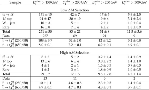
Sample ETmiss>150 GeV ETmiss>200 GeV ETmiss>250 GeV ETmiss>300 GeV
Low∆M Selection tt→ `` 131±15 42±7 17±5 5.6±2.5 1`top 94±47 30±19 9±6 3.1±2.4 W+jets 10±3 5±1 2±1 1.0±0.4 Rare 16±8 7±4 4±2 1.8±0.9 Total 251±50 83±21 31±8 11.5±3.6 Data 227 69 21 9 et→tχe 0 1(250/50) 108±3.7 32±2.0 12±1.2 5.2±0.8 et→tχe 0 1(650/50) 8.0±0.1 7.2±0.1 6.2±0.1 4.9±0.1 High∆M Selection tt→ `` 8±2 5±2 3.2±1.4 1.4±0.9 1`top 13±6 6±4 3.0±2.2 1.4±1.0 W+jets 4±1 2±1 1.5±0.5 0.9±0.3 Rare 4±2 3±1 1.8±0.9 1.0±0.5 Total 29±7 17±5 9.5±2.8 4.7±1.4 Data 23 11 3 2 et→tχe 0 1(250/50) 10±1.1 4.6±0.8 2.3±0.5 1.4±0.4 et→tχe 0 1(650/50) 4.9±0.1 4.7±0.1 4.3±0.1 3.7±0.1
9
Interpretation
The results of the search are interpreted in the context of models of top-squark pair production. As discussed in Section 3, we separately consider two possible decay modes of the top squark,
16 9 Interpretation [GeV] T M 0 50 100 150 200 250 300 Entries / 30 GeV 10 2 10 3 10 4 10 5 10 Data top l 1 ll → t t W+jets rare (250/50) 0 1 χ∼ t → t ~ SM + BDT1 Loose 0 1 χ∼ t → t ~ (a) -1 Ldt = 19.5 fb ∫ = 8 TeV, s CMS Data/MC 0.50 1 1.52 [GeV] T M 0 50 100 150 200 250 300 Entries / 60 GeV -1 10 1 10 2 10 3 10 Data top l 1 ll → t t W+jets rare (650/50) 0 1 χ∼ t → t ~ SM + BDT4 0 1 χ∼ t → t ~ (b) -1 Ldt = 19.5 fb ∫ = 8 TeV, s CMS Data/MC 0.50 1 1.52 BDT Output 0 0.2 0.4 Entries / 0.05 200 400 600 800 1000 1200 1400 1600 Data top l 1 ll → t t W+jets rare (250/50) 0 1 χ∼ t → t ~ SM + BDT1 Loose 0 1 χ∼ t → t ~ (c) -1 Ldt = 19.5 fb ∫ = 8 TeV, s CMS Data/MC 0 0.51 1.52 BDT Output 0.2 0.3 0.4 0.5 0.6 0.7 Entries / 0.10 0 5 10 15 20 25 30 Data top l 1 ll → t t W+jets rare (650/50) 0 1 χ∼ t → t ~ SM + BDT4 0 1 χ∼ t → t ~ (d) -1 Ldt = 19.5 fb ∫ = 8 TeV, s CMS Data/MC 0 0.51 1.52
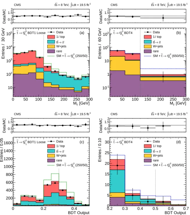
Figure 8: Comparison of data and MC simulation for the distributions of BDT output and MT corresponding to the tightest and loosest signal region selections in theet → tχe
0
1scenario. The MT distributions are shown after the requirement on the BDT output, and the BDT out-put distributions are shown after the MT > 120 GeV requirement (these requirements are also indicated by vertical dashed lines on the respective distributions). (a) MT after the loose cut on the BDT1 output; (b) MT after the cut on the BDT4 output; (c) BDT1 output after the MT cut; (d) BDT4 output after the MT cut. Expected signal distributions for mχe01 = 50 GeV and m
et = 250 GeV or 650 GeV are also overlayed, as indicated in the figures. In plot (b), the bin to the right of the vertical line contains all events with MT > 120 GeV, and has been scaled by a factor of 1/3 to indicate the number of events per 60 GeV. In all distributions the last bin contains the overflow.
[GeV] T M 0 50 100 150 200 250 300 Entries / 60 GeV 1 10 2 10 3 10 4 10 Data top l 1 ll → t t W+jets rare (250/50/0.5) ± 1 χ∼ b → t ~ SM + (x=0.5) BDT1 ± 1 χ∼ b → t ~ (a) -1 Ldt = 19.5 fb ∫ = 8 TeV, s CMS Data/MC 0 0.51 1.52 [GeV] T M 0 50 100 150 200 250 300 Entries / 60 GeV 1 10 2 10 3 10 Data top l 1 ll → t t W+jets rare (650/50/0.5) ± 1 χ∼ b → t ~ SM + (x=0.5) BDT3 ± 1 χ∼ b → t ~ (b) -1 Ldt = 19.5 fb ∫ = 8 TeV, s CMS Data/MC 0 0.51 1.52 BDT Output 0 0.1 0.2 0.3 0.4 0.5 Entries / 0.05 200 400 600 800 1000 Data top l 1 ll → t t W+jets rare (250/50/0.5) ± 1 χ∼ b → t ~ SM + (x=0.5) BDT1 ± 1 χ∼ b → t ~ (c) -1 Ldt = 19.5 fb ∫ = 8 TeV, s CMS Data/MC 0 0.51 1.52 BDT Output 0.2 0.3 0.4 0.5 0.6 0.7 Entries / 0.05 5 10 15 20 25 30 35 40 Data top l 1 ll → t t W+jets rare (650/50/0.5) ± 1 χ∼ b → t ~ SM + (x=0.5) BDT3 ± 1 χ∼ b → t ~ (d) -1 Ldt = 19.5 fb ∫ = 8 TeV, s CMS Data/MC 0 0.51 1.52
Figure 9: Comparison of data and MC simulation for the distributions of BDT output and MT corresponding to the tightest and loosest signal region selections in the x = 0.5et → bχe
+ sce-nario with an on-shell W boson. The MT distributions are shown after the requirement on the BDT output, and the BDT output distributions are shown after the MT >120 GeV requirement (these requirements are also indicated by vertical dashed lines on the respective distributions). (a) MT after the cut on the BDT1 output; (b) MT after the cut on the BDT3 output; (c) BDT1 output after the MT cut; (d) BDT3 output after the MT cut. Expected signal distributions for x = 0.5 with m
e
χ01 = 50 GeV and met = 250 GeV or 650 GeV are also overlayed, as indicated in the figures. In all distributions the last bin contains the overflow.
18 9 Interpretation
Table 5: The result of theet → bχe+ BDT analysis. For each signal region the individual back-ground contributions, total backback-ground, and observed yields are indicated. The uncertainty in-cludes both the statistical and systematic components. The expected yields for several example signal models are also indicated (statistical uncertainties only). The first number in parenthe-ses indicates the top-squark mass, the second the gluino mass, and the third the chargino mass parameter x. The units of the two mass values are GeV.
et→bχe +x=0.25 Sample BDT1 BDT2 BDT3 tt→ `` 18±4 2.2±1.3 1.2±1.0 1`top 10±5 4.0±1.8 1.5±0.8 W+jets 3±1 2.0±0.7 0.7±0.3 Rare 4±2 1.6±0.8 1.0±0.5 Total 35±6 9.8±2.4 4.4±1.4 Data 29 7 2 et→bχe +(450/50/0.25) 19±2.9 11±2.2 5.2±1.5 et→bχe +(600/100/0.25) 8.8±0.8 7.5±0.8 5.6±0.7 et→bχe + x=0.5
Sample BDT1 BDT2–Loose BDT2–Tight BDT3 BDT4
tt→ `` 40±5 21±4 4±2 6±2 100±16 1`top 24±10 15±7 4±3 4±2 33±12 W+jets 5±1 5±1 2±1 3±1 5±1 Rare 8±4 8±4 3±1 4±2 8±4 Total 77±12 50±9 13±4 17±4 146±21 Data 67 35 12 13 143 et→bχe +(250/50/0.5) 45±7.6 24±5.2 5.7±2.4 5.2±2.6 55±8.1 et→bχe +(650/50/0.5) 3.5±0.4 9.5±0.7 5.6±0.5 8.3±0.6 3.2±0.4 et→bχe +x=0.75 Sample BDT1 BDT2 BDT3 BDT4 tt→ `` 37±5 9±2 3.1±1.3 248±22 1`top 17±9 6±5 1.6±1.6 188±70 W+jets 4±1 4±1 1.6±0.6 22±6 Rare 4±2 4±2 1.8±0.9 20±10 Total 61±10 22±6 8.1±2.3 478±74 Data 50 13 5 440 et→bχe +(250/50/0.75) 115±13 21±5.6 8.0±3.7 518±28 et→bχe +(650/50/0.75) 3.9±0.4 8.4±0.6 6.8±0.6 5.5±0.5
et → tχe01 andet → bχe+ → bWχe01, each with 100% branching fraction. Using the results of Section 8, we compute 95% confidence level (CL) cross section upper limits for top-squark pair production in the m
e
χ01vs. metparameter space. Then, based on the expected pp→etet
∗production rate, these cross section limits are used to exclude regions of SUSY parameter space. For the et → bχe
+scenario, the mass of the intermediate e
χ±1 is specified by the parameter x defined in
Section 3.
In setting limits, we account for the following sources of systematic uncertainty associated with the signal event acceptance and efficiency. The uncertainty of the integrated luminosity deter-mination is 4.4% [62]. Samples of Z → ``events are used to measure the lepton efficiencies, and the corresponding uncertainties are propagated to the signal event acceptance and effi-ciency. These uncertainties are 3% for the trigger efficiency and a combined 5% for the lepton identification and isolation efficiency, where we also account for additional uncertainties in the modeling of the lepton isolation due to the differences in the hadronic activity in Z → ``and SUSY events. The uncertainty of the efficiency to tag bottom-quark jets results in an uncertainty for the acceptance that depends on model details but is typically less than 1%. The energy scale
Table 6: The result of theet → bχe+ cut-based analysis. For each signal region the individual background contributions, total background, and observed yields are indicated. The uncer-tainty includes both the statistical and systematic components. The expected yields for sev-eral sample signal models are also indicated (statistical uncertainties only). The first number in parentheses indicates the top-squark mass, the second the gluino mass, and the third the chargino mass parameter x. The units of the two mass values are GeV.
Sample EmissT >100 GeV EmissT >150 GeV EmissT >200 GeV EmissT >250 GeV
Low∆M Selection tt→ `` 875±57 339±23 116±14 40±9 1`top 658±192 145±70 41±24 14±9 W+jets 59±15 21±5 8±2 4±1 Rare 70±35 33±17 16±8 8±4 Total 1662±203 537±75 180±28 66±13 Data 1624 487 151 52 et→bχe +(450/50/0.25) 47±3.3 33±2.7 19±2.0 8.7±1.4 et→bχe +(600/100/0.25) 15±0.7 13±0.7 11±0.6 7.9±0.5 et→bχe +(250/50/0.5) 419±17 157±9.9 52±5.4 21±3.4 et→bχe +(650/50/0.5) 14±0.6 13±0.5 11±0.5 8.4±0.4 et→bχe +(250/50/0.75) 854±26 399±18 144±10 56±6.4 et→bχe +(650/50/0.75) 17±0.7 16±0.6 13±0.6 11±0.5 High∆M Selection tt→ `` 25±5 12±3 7±2 2.9±1.5 1`top 35±10 15±6 6±3 2.7±1.8 W+jets 9±2 5±1 2±1 1.8±0.6 Rare 9±5 7±3 4±2 2.4±1.2 Total 79±12 38±7 19±5 9.9±2.7 Data 90 39 18 5 et→bχe +(450/50/0.25) 30±2.7 23±2.3 15±1.8 7.3±1.3 et→bχe +(600/100/0.25) 11±0.6 9.7±0.6 8.4±0.6 6.1±0.5 et→bχe +(250/50/0.5) 37±4.8 23±3.8 11±2.6 5.0±1.7 et→bχe +(650/50/0.5) 11±0.5 9.8±0.5 8.6±0.4 6.7±0.4 et→bχe +(250/50/0.75) 32±5.2 23±4.4 11±2.9 3.6±1.4 et→bχe +(650/50/0.75) 9.2±0.5 8.4±0.5 7.5±0.4 6.3±0.4
of hadronic jets is known to 1–4%, depending on η and pT, yielding an uncertainty of 3–15% for the signal event selection efficiency. The larger uncertainties correspond to models for which the difference between the masses of the top squark and LSP is small.
The experimental acceptance for signal events depends on the level of ISR activity, especially in the small∆M region where an initial-state boost may be required for an event to satisfy the selection requirements, including those on Emiss
T , MT, and the number of reconstructed jets. The modeling of ISR in MADGRAPHis investigated by comparing the predicted and measured
pT spectra of the system recoiling against the ISR jets in Z+jets, tt, and WZ events. Good agreement is observed at lower pT, while the simulation is found to over predict the data by about 10% at a pT value of 150 GeV, rising to 20% for pT > 250 GeV. The predictions from the MC signal samples are weighted to account for this difference, by a factor of 0.8–1.0, depending on the pTof the system recoiling against the ISR jets, and the deviation of this weight from 1 is taken as a systematic uncertainty. Further details are given in Appendix B.
Upper limits on the cross section for top-squark pair production are calculated separately for each SR, incorporating the uncertainties of the acceptance and efficiency discussed above, using the LHC-style CLs criterion [63–65]. For each point in the signal model parameter space, the observed limit is taken from the signal region with the best expected limit. The results from the
20 9 Interpretation
BDT analysis are displayed in Fig. 10. The corresponding results from the cut-based analysis, and maps of the most sensitive signal regions for each of the top-squark decay modes, are presented in Appendix A.3. The cross section limits from the BDT analysis improve upon those from the cut-based analysis by up to approximately 40%, depending on the model parameters. Our results probe top squarks with masses between approximately 150 and 650 GeV, for neu-tralinos with masses up to approximately 250 GeV, depending on the details of the model. For theet → tχe01search, the results are not sensitive to the model points with m
et−mχe 0
1 = Mtop be-cause theχe
0
1 is produced at rest in the top-quark rest frame. However the results are sensitive to scenarios with m
et−mχe 0
1 < Mtop in which the top quark in the decayet → tχe 0
1 is off-shell, including regions of parameter space with the top squark lighter than the top quark.
The acceptance depends on the polarization of the top quarks in theet → tχe 0
1 scenario, and on the polarization of the charginos and W bosons in theet → bχe
+scenario. These polarizations depend on the left/right mixing of the top squarks and on the mixing matrices of the neutralino and chargino [36, 37]. The exclusion regions obtained in the nominalet → tχe
0
1 scenario with unpolarized top quarks are compared to those obtained with pure left-handed and pure right-handed top quarks in Fig. 11 (left). The limits on the top-squark andχe
0
1 masses vary by±10– 20 GeV depending on the top-quark polarization.
In theet → bχe
+ scenario, the acceptance depends on the polarization of the chargino, and on whether the Wχe
0 1 χe
±
1 coupling is left-handed or right-handed. In the nominal interpretations for theet → bχe
+models presented in Fig. 10, the signal events are generated with an unpolar-ized chargino and a left/right-symmetric Wχe
0 1 χe
±
1 coupling. We have studied the dependence of our results on these assumptions. We find that the scenarios in which the limits deviate the most from the nominal result correspond to right-handed charginos with either a right-handed Wχe
0 1 χe
±
1 coupling (maximum sensitivity) or a left-handed Wχe 0 1 χe
±
1 coupling (minimum sen-sitivity). This is shown for theet → bχe+ x = 0.5 model in Fig. 11 (right). The corresponding results for the x=0.25 and 0.75 scenarios can be found in Appendix A.3.
Mixed-decay scenarios, i.e., scenarios with non-zero top-squark decay branching fractions into bothet → tχe
0
1andet → bχe
+, have not been considered here. However, our results can be used to draw useful conclusions about these possibilities. We must distinguish between two typical SUSY spectra: one in which the chargino and LSP are nearly mass-degenerate, and the other in which the chargino is considerably heavier. In the degenerate case, corresponding to x ≈0, the acceptance is small for top-squark pairs with one or moreet→bχe+decays. This is because the visible decay products in theχe
+
1 → χe 0
1+X process are soft and likely to escape detection. Thus, to a good approximation, in these scenarios the top-squark pair cross section limit can be extracted by scaling the corresponding limit in the 100%et →tχe
0
1model byB2, whereBis the branching fraction foret→tχe
0
1. Exclusion regions for a few choices ofBare shown in Fig. 12. In the mixed case with a chargino much heavier than the LSP, a conservative approximate cross section limit can be obtained as σ(pp→etet∗) <min(σ0/B
2
, σ+/(1− B)2), where σ0and σ+are the cross section limits for the 100%et →tχe01and 100%et →bχe+scenarios, respectively, andB is the branching fraction defined above. (The limits σ0 and σ+shown in Fig. 10 are available electronically [66].) This approach is conservative as it uses only one out of the three possible decay modes of the top-squark pair. It should also be noted that in the heavier-chargino sce-nario it is possible for one additional neutralino (χe
0
2) to be nearly degenerate with the chargino. The decayet → tχe
0
2 followed by, for example,χe 0
2 → Zχe 0 1or Hχe
0
1 would then also be possible. This would further complicate the interpretation of the experimental results.
[GeV] t ~ m 100 200 300 400 500 600 700 800 [GeV]0 1 χ∼ m 0 50 100 150 200 250 300 350 400 upper limit [pb] σ -3 10 -2 10 -1 10 1 10 2 10 unpolarized top BDT analysis 0 1 χ ∼ t → t ~ *, t ~ t ~ → pp Observed (±1σtheory) ) σ 1 ± Expected ( -1 Ldt = 19.5 fb ∫ = 8 TeV, s CMS W = m 1 0 χ ∼ - mt ~ m t = m 1 0 χ ∼ - mt ~ m [GeV] t ~ m 200 300 400 500 600 700 800 [GeV] 1 0 χ∼ m 0 50 100 150 200 250 300 350 400 upper limit [pb] σ -3 10 -2 10 -1 10 1 10 2 10 BDT analysis + 1 χ ∼ b → t ~ *, t ~ t ~ → pp Observed (±1σtheory) ) σ 1 ± Expected ( 0 1 χ ∼ + 0.75 m t ~ = 0.25 m ± 1 χ ∼ m -1 Ldt = 19.5 fb ∫ = 8 TeV, s CMS W = m 0 1 χ ∼ - m ± 1 χ ∼ m [GeV] t ~ m 300 400 500 600 700 800 [GeV]0 1 χ∼ m 0 50 100 150 200 250 300 350 400 upper limit [pb] σ -3 10 -2 10 -1 10 1 10 2 10 BDT analysis + 1 χ ∼ b → t ~ *, t ~ t ~ → pp Observed (±1σtheory) ) σ 1 ± Expected ( 0 1 χ ∼ + 0.5 m t ~ = 0.5 m ± 1 χ ∼ m -1 Ldt = 19.5 fb ∫ = 8 TeV, s CMS W = m 0 1 χ ∼ - m ± 1 χ ∼ m [GeV] t ~ m 200 300 400 500 600 700 800 [GeV] 1 0 χ∼ m 0 50 100 150 200 250 300 350 400 upper limit [pb] σ -3 10 -2 10 -1 10 1 10 2 10 BDT analysis + 1 χ ∼ b → t ~ *, t ~ t ~ → pp Observed (±1σtheory) ) σ 1 ± Expected ( 0 1 χ ∼ + 0.25 m t ~ = 0.75 m ± 1 χ ∼ m -1 Ldt = 19.5 fb ∫ = 8 TeV, s CMS W = m 0 1 χ ∼ - m ± 1 χ ∼ m
Figure 10: Interpretations using the primary results from the BDT method. (a)et → tχe 0 1model; (b)et → bχe + model with x = 0.25; (c) et → bχe + model with x = 0.50; (d) et → bχe + model
with x =0.75; The color scale indicates the observed cross section upper limit. The observed, median expected, and±1 standard deviation (σ) expected 95% CL exclusion contours are indi-cated. The variations in the excluded region due to±1σ uncertainty of the theoretical predic-tion of the cross secpredic-tion for top-squark pair producpredic-tion are also indicated.