Convolutional Neural Networks for Transient Candidate
Vetting in Large-Scale Surveys
Fabian Gieseke,
1,2
?
Steven Bloemen,
3,4
Cas van den Bogaard,
1
Tom Heskes,
1
Jonas Kindler,
5
Richard A. Scalzo,
6,7,8
Val´
erio A.R.M. Ribeiro,
3,9,10,11
Jan van Roestel,
3
Paul J. Groot,
3
Fang Yuan,
6,7
Anais M¨
oller,
6,7
Brad E. Tucker,
6,7
1Institute for Computing and Information Sciences, Radboud University, P.O. Box 9010, 6500 GL Nijmegen, The Netherlands 2Department of Computer Science, University of Copenhagen, Sigurdsgade 41, 2200 Copenhagen, Denmark
3Department of Astrophysics/IMAPP, Radboud University, P.O. Box 9010, 6500 GL Nijmegen, The Netherlands 4NOVA Optical InfraRed Instrumentation Group, Oude Hoogeveensedijk 4, 7991 PD Dwingeloo, The Netherlands 5Institute of Cognitive Science, University of Osnabr¨uck, Wachsbleiche 27, 49090 Osnabr¨uck, Germany
6Research School of Astronomy and Astrophysics, Australian National University, Canberra, ACT 2611, Australia 7ARC Centre of Excellence for All-Sky Astrophysics (CAASTRO), Australia
8Centre for Translational Data Science, University of Sydney, Darlington, NSW 2008, Australia
9CIDMA, Departamento de F´ısica, Universidade de Aveiro, Campus de Santiago, 3810-193 Aveiro, Portugal 10Instituto de Telecomunica¸c˜oes, Campus de Santiago, 3810-193 Aveiro, Portugal
11Department of Physics and Astronomy, Botswana International University of Science and Technology, Private Bay 16, Palapye, Botswana
Accepted XXX. Received YYY; in original form ZZZ
ABSTRACT
Current synoptic sky surveys monitor large areas of the sky to find variable and transient astronomical sources. As the number of detections per night at a single telescope easily exceeds several thousand, current detection pipelines make intensive use of machine learning algorithms to classify the detected objects and to filter out the most interesting candidates. A number of upcoming surveys will produce up to three orders of magnitude more data, which renders high-precision classification systems essential to reduce the manual and, hence, expensive vetting by human experts. We present an approach based on convolutional neural networks to discriminate between true astrophysical sources and artefacts in reference-subtracted optical images. We show that relatively simple networks are already competitive with state-of-the-art systems and that their quality can further be improved via slightly deeper networks and additional preprocessing steps – eventually yielding models outperforming state-of-the-art systems. In particular, our best model correctly classifies about 97.3% of all “real” and 99.7% of all “bogus” instances on a test set containing 1,942 “bogus” and 227 “real” instances in total. Furthermore, the networks considered in this work can also successfully classify these objects at hand without relying on difference images, which might pave the way for future detection pipelines not containing image subtraction steps at all.
Key words: surveys – techniques: image processing – methods: data analysis – supernovae: general
1 INTRODUCTION
A number of large optical survey telescopes such as Skymap-per (Keller et al. 2007), the Palomar Transient Fac-tory (PTF, Rau et al. 2009), and Pan-STARSS1 (Kaiser et al. 2010) are searching for transient events. New
genera-? E-mail: [email protected]
tion surveys will be able to scan large amounts of the sky faster and deeper allowing searches for extremely rare or hitherto undiscovered events, such as possible electromag-netic counterparts of gravitational wave sources (see, e. g.,
Nissanke et al. 2013;Smartt et al. 2016). Those surveys will increase our statistical samples of more common events, such as supernovae, for experiments in cosmology and
tal physics (Riess et al. 1998;Schmidt et al. 1998;Perlmutter et al. 1999).
The detection of rare transient events among the vast majority of relatively constant sources is an important yet challenging task. Most surveys use difference imaging to find variable stars and transients. This is usually achieved by per-forming a pixel-by-pixel subtraction of a pre-existing tem-plate image from the image of interest. Astrophysical sources that are variable or were absent in the template image re-main, while constant sources – which represent the vast ma-jority of the detected sources – are removed at the pixel level. During the difference imaging process, the template image is aligned and resampled to take into account distortions in the target image, and a convolution is done to match the point-spread function in all regions of the image (see, e. g.,
Alard & Lupton 1998;Alard 2000).
While this process, in principle, allows one to very ef-ficiently find rare transient events, in practice many of the resulting images contain a large number of “bogus” objects. These “bogus” objects trigger source finding algorithms, but rather than being of astrophysical nature, they are, in re-ality, artefacts. Such artefacts can result from a variety of processes such as issues with image processing (e. g., bad alignment at the subtraction step, between the template and target images), detector imperfections, atmospheric disper-sion and cosmic rays passing through the detector.
The number of potential detections can be very large, with thousands of events per night produced by current syn-optic surveys, and millions of detections per night expected from future surveys such as the Large Synoptic Sky Sur-vey (LSST,Ivezic et al. 2008). The classification of the de-tections as either “real” or “bogus” sources is a necessary but daunting task, which will become an even more seri-ous problem in the future. Manual verification by humans is expensive and, most likely, impossible to conduct for the amounts of data expected. For this reason, automatic de-tection algorithms that yield both a high purity and a high completeness will play an essential role for future transient surveys.
Machine learning aims at constructing models that can perform classification tasks in an automatic manner (Hastie et al. 2009;Murphy 2012). One particular subfield of ma-chine learning techniques, called deep learning (LeCun et al. 2015), has gained considerable attention during the past few years. Deep learning algorithms have successfully been ap-plied to a variety of real-world tasks. Two recent trends have sparked the interest in such algorithms: (1) the dramatic in-crease of data volumes in almost any field, which, in turn, has produced a massive amount of labelled data that can be used to train and evaluate the models; and (2) the enormous increase in compute power, particularly due to massively-parallel devices such as graphics processing units (GPUs), which led to a significant reduction of the practical runtime needed to generate deep architectures (Coates et al. 2013).
This paper aims at improving the automatic identifica-tion of transient sources in astronomical images. A stan-dard approach, usually implemented in current detection pipelines, is based on extracting features from photomet-ric images, such as the fluxes of the detected sources. Given such a representation of the objects at hand, one resorts to well-established machine learning algorithms. The most widely used approaches are currently based on some kind of
dimension reduction (e.g., by conducting a principal com-ponent analysis in the preprocessing phase or by extracting physically-motivated features such as magnitudes or param-eters that reflect the shape of the point spread function) and a subsequent application of classification methods such as random forests, support vector machines, nearest neighbour techniques, or (standard) artificial neural networks (e. g.,
Bloom et al. 2012;Brink et al. 2013;Goldstein et al. 2015;
Morii et al. 2016;Wright et al. 2015;Buisson et al. 2015). Some recent works also resort to deep neural networks (here, the term “deep” refers to the number of hidden layers in a network, see Section2for details). For example, a recent ap-proach resorts to a neural network with three hidden layers that is applied given physically-motivated features (Morii et al. 2016). Another approach is based on recurrent neural networks with up to two hidden layers, given time series data that stems from flux values extracted from different obser-vations (Charnock & Moss 2016). Note that these schemes also resort to an explicit feature extraction step that is con-ducted in the preprocessing phase.
This paper focuses on improving current detection pipelines and classification systems by means of convolu-tional neural networks (LeCun et al. 1989,2015). In contrast to “standard” deep architectures, convolutional neural net-works do not rely on a feature extraction step conducted in the preprocessing phase. Instead, these models “learn” good features based on the raw input image data. While convolu-tional neural networks have already been considered in the context of astronomy (Dieleman et al. 2015b;Kim & Brun-ner 2016), we present the first application of such models for the task of transient vetting. In this paper we make use of a dataset compiled in the framework of the Skymapper supernova searches (Scalzo et al. 2017).
2 BACKGROUND
In this section, we provide some machine learning back-ground related to the techniques used in this work.
2.1 Random Forests Revisited
Random forests depict ensembles of individual classification trees (Breiman 2001; Hastie et al. 2009;Murphy 2012). In general, ensemble methods are among the most successful models in machine learning. This is especially true for ran-dom forests, which often yield high accuracies while being, at the same time, conceptually very simple and resilient against small changes of the involved parameter assignments. Since their introduction more than a decade ago, random forests have been extended and modified in various manners. A standard random forest consists of many individual trees (e. g., classification or regression trees), where each tree is built in a slightly “different” way (see below) and the ensem-ble combines the benefits of all of them, see Figure1.
The trees of a random forest are usually constructed in-dependently from each other. Each tree is built from top to bottom, where the root corresponds to all training instances and the leaves to subsets of the training data. During the construction, each internal node is recursively split into two children such that the resulting subsets exhibit a higher “pu-rity”. The overall process stops as soon as the leaves are
(a) Tree 1 (b) Tree 2 (c) Tree 3 Figure 1. A random forest built for 50 training points. Each tree of the ensemble is built from top to bottom and at each node, slightly different “splits” are used – resulting in different tree structures. The construction takes place until the leaves are pure, meaning that only patterns belonging to the same class are given in a single leaf (resulting in less than 50 leaves in this case). For splitting up the nodes, one resorts to different criteria such as the mean squared error for regression scenarios or the Gini index for classification tasks. A random forecasts combines the predictions made by the individual trees.
“pure” (i. e., they only contain patterns with the same label) or as soon as some other stopping criterion is fulfilled. The original way of building a random forest is based on subsets of the training patterns, one subset for each tree to be built, called bootstrap samples (Breiman 2001). These subsets are drawn uniformly at random (with replacement) to obtain slightly different training sets and, hence, trees.
The quality of a node split is measured in terms of the gain in purity, which, in turn, is measured via differ-ent metrics depending on the desired outcome. Typical met-rics include, for example, the mean squared error for the regression case or the Gini index for classification prob-lems (Breiman 2001). For example, a pure split would be one yielding children containing only instances belonging to the same class, therefore, no further splits are required (Breiman 2001;Hastie et al. 2009;Murphy 2012).
Given a new, unseen instance, one can obtain a predic-tion for each single tree by traversing the tree from top to bottom based on the splitting information stored in the in-ternal nodes until a leaf node is reached. The labels stored in this leaf are then combined to obtain the prediction for a single tree (e. g., by considering the mean for regression sce-narios). The overall prediction of the random forest is based on a combination of the individual predictions. For regres-sion scenarios, one usually simply averages the predictions. For classification settings, one can resort to a majority vote. In summary, the individual trees of a random forest can be seen as “different” experts, whose opinions are combined to obtain a single overall prediction for a new instance.
2.2 Deep Convolutional Neural Networks
Below we briefly introduce convolutional neural networks. For a more detailed description, we refer the reader to the excellent overview by LeCun et al. (2015) and the articles with applications to astronomical research (e.g., Dieleman et al. 2015b;Kim & Brunner 2016).
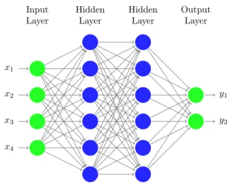
x1 x2 x3 x4 y1 y2 Hidden Layer Hidden Layer Input Layer Output Layer
Figure 2. A standard fully-connected artificial neural network with two hidden layers. The nodes of the network are called neu-rons and the output of each neuron corresponds to the weighted sum of its input neurons, transformed by an activation function. The output layer contains one neuron for each class and, given an input instance, outputs the corresponding class probabilities (in the case of classification scenarios).
2.2.1 Artificial Neural Networks
Convolutional neural networks are special types of the stan-dard artificial neural networks (ANNs) (Hastie et al. 2009;
Murphy 2012), which, in turn, consist of collections of in-terconnected nodes. In a nutshell, a multilayered artificial neural network is based on several layers, where the output of a given layer serves as input for the next layer. The first layer is called the input layer and the last layer the output layer. In between, there requires at least on hidden layer. For standard artificial neural networks, these layers are fully connected, meaning that all nodes of a given layer are con-nected to all nodes of the next layer (Figure2).1
The input layer is specified via the available input data. For example, given a feature vector x ∈ Rd extracted from an image (e. g., a set of magnitudes), each of the feature values x1, . . . , xdcorresponds to one of the input nodes of the input layer. Similarly, the output layer is determined by the learning task at hand. For a binary classification problem (e. g., “bogus” vs. “real”), the output layer consists of two nodes that, for a given input instance, eventually output the class probabilities for each of the classes (note that in this special case, a single output node is sufficient since the classes are mutually exclusive).
The output of the first hidden layer is obtained via the weights W1associated with the connections between the in-put layer and the first hidden layer. More specifically, the output of layer j is given by the transformation rule
xj = f (Wjxj−1+ bj), (1)
where Wj is the weight matrix associated with the
connec-tions between layer j − 1 and j, bj a vector containing so-called bias values associated with layer j, and f : RK → RK
1 For convolutional neural networks, this is usually not the case except for the last layers (see below).
a so-called activation function with K being the total num-ber of neurons in layer j. Note that the transition from layer j −1 to j basically corresponds to applying a standard linear model followed by an element-wise application of the acti-vation function f (Hastie et al. 2009; Murphy 2012). The dimensions of all involved vectors and matrices depend on the number of nodes and connections between the nodes. For example, for the transition from the input to the first hid-den layer in Figure2, we have x0∈ R4, x1∈ R6, W1∈ R6×4,
and b1 ∈ R6. Popular choices for the activation function f: RK → RK are
• the linear activation function [ f (x)]i= xi,
• the rectified activation function [ f (x)]i = max(0, xi), • or the softmax activation function [ f (x)]i=ÍKexi
j=1ex j
for i = 1, . . ., K. Hence, the layers of a neural network iter-atively transform the feature representation x ∈ Rd of an input instance. Finally, the vector at the last hidden layer is transformed to only a single output neuron for standard regression scenarios or to multiple output neurons for clas-sification or multivariate regression scenarios. Note that the different layers can resort to different activation functions, except for the last one, the output layer, which is some-what restricted by the learning task at hand. For regres-sion tasks, one usually makes use of a linear activation func-tion, whereas the softmax activation function is a common choice for classification scenarios. Hence, given a new in-stance x ∈ Rdfor which one would like to obtain a prediction (e. g., if it is of type “bogus” or “real”), one consecutively ap-plies the transformation rule (Equation1), which eventually yields the output vector y. For regression scenarios, y ∈ R1 corresponds to the prediction made by the network for the input x, whereas the vector y ∈ RC contains the class proba-bilities given classification scenarios with C possible classes. Training such a neural network basically corresponds to finding weights such that the network performs well on new, unseen data (e. g., fewer misclassifications). Various op-timization techniques can be applied (e. g., variants of gradi-ent descgradi-ent) so that the output of the network becomes more consistent with the class labels given for the training data. The so-called learning rate γ > 0 is a parameter used by many of the underlying optimisation techniques that affects the size of the weight updates (e. g., similar to the step-size of standard gradient descent). The learning rate is a parameter that needs to be specified beforehand (as the network struc-ture itself) and is usually tuned via grid search (i. e., various assignments are tested and one resorts to the training data to evaluate the induced quality).
Another important parameter is the number of epochs, which usually correspond to a full pass over the available training data or to processing a certain batch of a fixed size of training instances (most optimisation techniques process the training instances iteratively). For the latter option, the batch size determines the number of instances processed per single epoch (Hastie et al. 2009).
2.2.2 Convolutional Neural Networks
In recent years, so-called deep networks have become more and more popular. Here, the term “deep” is related to the number of hidden layers. A special type of such deep
archi-tectures are convolutional neural networks, which consist of multiple layers of different types. Such networks have been successfully applied in the context of many application do-mains. We will focus on image-based input data for the de-scription of convolutional neural networks.
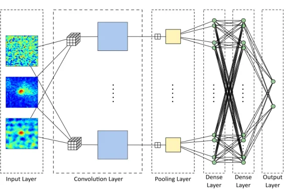
A typical convolutional neural network with multiple hidden layers is shown in Figure 3. As standard artificial networks, convolutional neural networks also exhibit an in-put and an outin-put layer. Furthermore, the last hidden layers often correspond to standard fully-connected dense layers as well. In contrast, the first hidden layers are conceptually very different and consist of various types of layers. The most prominent types, applied in this work, are convolutional lay-ers, pooling laylay-ers, and dropout layers:
• Convolutional layers: Such layers form the basis for con-volutional neural networks and yield so-called feature maps by sliding a small window of weights across the input feature maps that stem from the previous layer (the input images of the input layer form the initial feature maps). In a nutshell, each feature map of a given layer stems from convolving all input feature maps using a set of filters (weight matrices), one filter for each input feature map. For example, in Fig-ure3, we have, for each feature map in the first hidden layer, three filters of size 3 × 3 that are used to convolve all three input feature maps. The sum of all these convolved images correspond to the term Wjxj−1in equation (1). Afterwards,
a matrix of bias values is added to this sum image, followed by an element-wise application of an activation function f .
• Pooling layers: This is the second prominent type of lay-ers. Pooling layers are used to decrease the number of learn-able parameters (the filters/weight matrices). More pre-cisely, such a pooling layer reduces the sizes of the fea-ture maps by aggregating pixel values. For example, a max-pooling layer considers patches within each feature map and replaces each patch by the maximum value in that patch (e. g., in Figure3, each feature map of the previous layer is processed via patches of size 2 × 2, leading to new feature maps of half the size). Naturally, other operations can be applied such as taking the mean of a given pixel patch.
• Dropout layers: These guard against overfitting, in which the trained network relies heavily on aspects of the training data that do not generalise well to new, unseen data. Dropout layers randomly omit hidden units by setting their value to zero with a user-defined probability p ∈ (0, 1) such that other hidden units cannot fully rely on them (such tech-niques are also used in standard artificial neural networks). Thus, these layers force the network to rely on more units, preventing a reliance on noise or artefacts (dropout layers are not shown in Figure3 since dropout basically only af-fects the underlying optimisation process).
Therefore, convolutional layers aim to extract features that are somewhat invariant against translation. Note that there are also significantly less weights/connections for such convolutional layers (only the values given in the fil-ters/weight matrices have to be learnt). Similarly, pooling layers make the network invariant against small transitions and reduce the number of nodes in the network (i. e., pixels in the feature maps). These two modifications often signif-icantly increase the classification performance of such net-works compared to standard fully-connected artificial neural networks.
Convolu�on Layer Pooling Layer Dense Layer Dense Layer Output Layer Input Layer
Figure 3. A convolutional neural network with one convolutional and one pooling layer, followed by two fully connected standard hidden layers and an output layer. Prior to the fully-connected hidden layers, the pixel-based feature maps are flattened, meaning that all pixel values of all feature maps of the previous layers are concatenated to form a single vector. Generally, by resorting to multiple convolutional and pooling layers, convolutional neural networks are capable of learning a hierarchical feature representation of the input instances – starting with simple features at early layers and more complex features towards the end.
3 DEEP TRANSIENT DETECTION
In this section we provide details of the different models considered for this paper in order to detect transients.
3.1 Imaging Data
Our models were trained on early science operations, prior to April 2015, imaging data from the Skymapper Supernova and Transient Survey. The difference imaging pipeline is de-scribed in more detail in (Scalzo et al. 2017). The main image processing tools used are the SWarp (Bertin et al. 2002) for astrometric registration and resampling to a common coor-dinate system, SExtractor (Bertin & Arnouts 1996) for source detection and photometry, and HOTPANTS2 for photometric registration and image subtraction. Data for each example include the template image, the target image, and the difference image. In Figure 4we show examples of both “real” and “bogus” taken from the dataset.
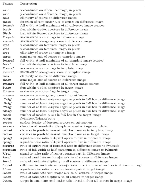
We trained our random forest models on features ex-tracted from the images (Table1), while the convolutional neural networks were applied directly on the images them-selves. To evaluate the performance of each model, we split the available data into a training set and a test set of roughly equal size.
To make the most of our limited number of “real” train-ing instances, we enabled traintrain-ing on multiple distinct detec-tions of the same transient candidate on different nights; this allowed us to sample more real variation in seeing and sky background level for the same candidate than we would if we
2 http://www.astro.washington.edu/users/becker/v2.0/hotpants.html
included only one detection of each candidate. Because we expected the classifier results to also be affected by details of the host galaxy placement and morphology, which would be the same for multiple observations of the same transient, we placed all observations of the same object (e. g., a super-nova) within the same partition (i. e., training or test); this choice enables our training methodology to make honest es-timates of the generalization error to entirely new transient sources with different host galaxy properties. Apart from this constraint, the partition each individual transient can-didate occupied was chosen at random. The training set con-tains 2,237 instances (2,010 “bogus” and 227 “real”) of 851 distinct “bogus” and 140 distinct “real” sky objects. The test set contains 2,236 instances (2,009 “bogus” and 227 “real”) of 851 distinct “bogus” and 141 distinct “real” sky objects.
We removed those instances that were located less than 15 pixels from the edge of a CCD, in both the training and test sets, since the pixel cut-outs we use for our analysis (see Section3.3) would be incomplete in these cases. This yields a final training set with 2,162 instances (1,939 “bogus” and 223 “real”) and a test set containing 2,169 instances (1,942 “bogus” and 227 “real”).
3.2 Baseline: Random Forests & Features
For the use of random forests, we extract various features from the imaging data (see Table1). Most of the features are taken fromBloom et al.(2012). A large fraction of the fea-tures reflect properties of the source in the difference image, as well as some contextual information such as the presence of, and distance from, a nearby neighbour in the template image (Bloom et al. 2012). We supplemented the features
Table 1. Features used as input for the random forest models.
Feature Description
xsub x coordinate on difference image, in pixels ysub y coordinate on difference image, in pixels esub ellipticity of source on difference image
thsub direction of semi-major axis of source on difference image fwhmsub full width at half maximum of all difference image sources f4sub flux within 4-pixel aperture in difference image
f8sub flux within 8-pixel aperture in difference image flagsub sextractor source flags in difference image starsub sextractor star-galaxy score in difference image xref x coordinate on template image, in pixels yref x coordinate on template image, in pixels eref ellipticity of source on template image thref semi-major axis of source on template image
fwhmref full width at half maximum of all template image sources f4ref flux within 4-pixel aperture in template image
flagref sextractor source flags in template image starref sextractor star-galaxy score in template image enew ellipticity of source on difference image
thnew semi-major axis of source on difference image
fwhmnew full width at half maximum of all target image sources f4new flux within 4-pixel aperture in target image
flagnew sextractor source flags in target image starnew sextractor star-galaxy score in target image
n2sig3 number of at least 2-sigma negative pixels in 3x3 box in difference image n3sig3 number of at least 3-sigma negative pixels in 3x3 box in difference image n2sig5 number of at least 2-sigma negative pixels in 5x5 box in difference image n3sig5 number of at least 3-sigma negative pixels in 5x5 box in difference image nmask number of masked pixels in 5x5 box in the target image
Rfwhm fwhmnew/fwhmref ratio
goodcn surface density of detected sources on subtraction
subconv direction of convolution (template-target or target-template) nndref distance in pixels to nearest neighbour source in template image nndnew distance in pixels to nearest neighbour source in target image apsig4 signal-to-noise ratio of 4-pixel aperture flux in difference image apsig8 signal-to-noise ratio of 4-pixel aperture flux in difference image normrms ratio of square root of isophotal area in difference image to fwhmsub normfwhm ratio of full width at half maximum in difference image to fwhmsub Rfref signal-to-noise ratio of nearest counterpart in difference image Raref ratio of candidate semi-major axis to all sources in difference image Reref ratio of candidate ellipticity to all sources in difference image
Dthref difference in candidate semi-major axis direction from all sources in difference image Rfnew signal-to-noise ratio of nearest counterpart in target image
Ranew ratio of candidate semi-major axis to all sources in target image Renew ratio of candidate ellipticity to all sources in target image
Dthnew target in candidate semi-major axis direction from all sources in target image
above with new features intended to capture the global prop-erties of the images - these flag obviously bad (e. g., trailed) images and subtractions. We also included SExtractor er-ror codes and star-galaxy separation scores; the latter pro-vide a redundant output from a different method (neural network) that may capture aspects of point sources not cov-ered by our existing features.
As with many other machine learning models, the clas-sification performance depends on the particular parameter assignments used to generate the random forest. However, random forests are usually very robust against small modi-fications, i. e., given reasonable parameter assignments, the validation performance is often very similar. The main pa-rameters that need to be tuned are: (1) the number of es-timators, (2) the number of features tested per split, (3)
if bootstrap samples are used or not, and (4) the stopping criterion used. Furthermore, variations of classical random forests exist such as the extremely randomised trees (Geurts et al. 2006), which consider “random” thresholds as potential splitting candidates.
For our analysis, we have tested different random for-est variants and parameter assignments. However, for sim-plicity, we only report results of a single configuration (all others yielded very similar performances). In particular, we consider the Gini index to measure the impurity of the inter-nal node splits, make use of 500 trees built using a bootstrap sample, resort to fully-grown trees, and test√d features per node split, where d is the number of overall features
consid-(a) Bogus (b) Real
Figure 4. “Best” case examples of three “bogus” and three “real”. The columns represent the template, target, and difference images per field (from left to right) and the rows represent different fields. The different colours along with the colour bars illustrate the pixel intensities per image. For “real” sources, there is usually no flux in the centre on the template image. However, there may be “misleading” instances very close to the centre of the image (which, ideally, would no longer be present in the difference image). The majority of the instances in the dataset are simple cases. As shown in our experiments, there is still a significant number of difficult instances outstanding, which can be very challenging for machine learning models to identify correctly. The unit of the colour scale is in counts.
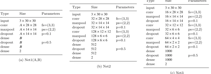
Type Size Parameters
input 3 × 30 × 30 conv A ×28 × 28 fs=(3,3) maxpool A ×14 × 14 ps=(2,2) dropout A ×14 × 14 p=0.1 dense B dropout B p=0.5 dense B dense 2 (a) Net1(A,B)
Type Size Parameters
input 3 × 30 × 30 conv 32 × 28 × 28 fs=(3,3) maxpool 32 × 14 × 14 ps=(2,2) dropout 32 × 14 × 14 p=0.1 conv 128 × 12 × 12 fs=(3,3) maxpool 128 × 6 × 6 ps=(2,2) dropout 128 × 6 × 6 p=0.1 dense 512 dropout 512 p=0.5 dense 512 dense 2 (b) Net2
Type Size Parameters
input 3 × 30 × 30 conv 16 × 28 × 28 fs=(3,3) maxpool 16 × 14 × 14 ps=(2,2) dropout 16 × 14 × 14 p=0.1 conv 32 × 12 × 12 fs=(3,3) maxpool 32 × 6 × 6 ps=(2,2) dropout 32 × 6 × 6 p=0.1 conv 64 × 4 × 4 fs=(3,3) maxpool 64 × 2 × 2 ps=(2,2) dropout 64 × 2 × 2 p=0.1 dense 1000 dropout 1000 p=0.5 dense 1000 dense 2 (c) Net3
Table 2. Network structures considered in this work (‘fs’ denotes the filter size of the convolutional layer, ‘ps’ the pooling size of the pooling layer and ‘p’ the dropout probability). A and B are parameters determining the input sizes of the layers.
ered.3 We also tested various other parameter assignments, which all yielded very similar classification accuracies (as long as a sufficiently large amount of trees was considered).
3 We use
Python 2.7 and the scikit-learn package (version 0.18) (Pedregosa et al. 2011) for processing and analysing the data. More precisely, we make use of the sklearn.ensemble.RandomForestClassifier class as the random forest implementation and initialise the model using the following parameters: bootstrap=True, n_estimators=500, min_samples_split=2, criterion="gini", and max_features="sqrt".
3.3 Network Structures & Parameters
While convolutional neural networks have been success-fully applied to several real-world tasks (see, e. g., LeCun et al. 2015), choosing the best-performing network structure (w.r.t. the classification performance on the test set) is often based on trial-and-error. Very deep structures might be dis-advantageous given “simple tasks”. On the other hand, too simplistic structures might not be able to adapt to the learn-ing task at hand and, thus, may yield unsatisfactory results as well. Therefore, the goal is to consider models that are complex enough to capture the characteristics of a learning task and that are, at the same time, not too complex. This is
related to the so-called bias-variance tradeoff (Hastie et al. 2009), which describes the well-known problem in machine learning of finding models with the right complexity such that they perform well on unseen data, and to the optimi-sation process itself. For example, deeper models generally exhibit more model parameters that need to be tuned/fitted, whereas in shallower networks one usually tunes less parame-ters. In this paper, we tackled this problem by starting with very simple and shallow convolutional networks and then increasing the complexity of the networks step-wise adding further convolutional layers. As will be shown in our ex-perimental evaluation, simple convolutional neural networks already yield very promising classification results. Further-more, due to their simplicity, one gains insight into how and why these networks perform so well. Additionally, the per-formance may be improved by means of data augmentation and further preprocessing steps.
The network structures considered in this paper are pre-sented in Table 2. Unless stated otherwise, the input lay-ers correspond to the three input images that are available (i. e., template, target, difference). Each network contains at least one max-pooling, convolutional, and dropout layers. The final layers are fully connected, followed by a softmax activation function to obtain class probabilities (“bogus” vs. “real”). The corresponding parameters for each layer are pro-vided in the table. We considered 1,000 training iterations for all networks without any data augmentation (see be-low) and 5,000 for the ones with data augmentation. Here, a training iteration refers to processing a batch of 128 training images.
For the convolutional neural network approaches, we cropped the images to a size of 30 × 30 pixels and made use of the Python package nolearn (version 0.6.1.dev0).4 More precisely, we made use of the nolearn.lasagne.NeuralNet class and initialised the models with different parameters and layers (see Table2). We complemented Net2 and Net3 with data augmentation steps that were conducted on-the-fly per training iteration (i.e., per batch of 128 training in-stances). In particular, we rotated each image by 90◦, 95◦, 100◦, 180◦, 185◦, 190◦, 270◦, 275◦, and 280◦. Subsequently, all “real” instances were flipped horizontally and vertically. Note that we did not apply any translation augmentation step since it is guaranteed that all “real” instances are cen-tred (up to 1 or 2 pixels).5 Resampling of the augumented images was done in a manner to perserve the flux using the scipy.ndimage.interpolation.rotate function. Since the data augumentation step essentially yields a significantly larger dataset, we increased the number of training iterations (5,000 instead of 1,000). For all networks, we resorted to the nolearn default settings to initialise the weights of all layers (i.e., Glorot with uniformly sampled weights) (Glorot & Ben-gio 2010). Furthermore, to train the networks, we resorted to Adam updates with learning rateγ = 0.0002 (Kingma &
4 The nolearn package implements various wrappers for the Lasagne package, which, in turn, depicts a lightweight library for the well-known Theano package (see,Nouri 2014;Dieleman et al. 2015a;Theano Development Team 2016, for details).
5 We also conducted some experiments with very small transla-tion steps, which, however, did not lead to an improvement w.r.t. the classification performance.
Ba 2014). The overall process aimed to minimise the cat-egorical cross entropy as objective with L2 regularisation (objective_lambda2=0.025).
We made use of standard low-cost gaming graphics pro-cessing units (GPUs), such as Nvidia GeForce GTX 770, to speed up the training and validating processes. Training the models was the most time-consuming phase of the two pro-cesses. Here, each training iteration (i.e., processing a batch of 128 images) took about 0.5 to 5 seconds depending on the network architecture and the particular GPU being used. Note, however, that the network models considered in this work can all be generated in a couple of minutes (e.g., 1000 training iterations for the shallow networks) or hours (e.g., 5000 training iterations and the deeper networks).
4 ANALYSIS
We compared the performance of the random forests ap-proach, currently used in data processing pipelines, with those of different convolutional neural networks described above.
4.1 Experimental Setup
All experiments resorted to data described in Section 3.1
to generate and evaluate the models. In the following, we assume that the label for a “real” instance is +1 and the one for a “bogus” instance is −1. We split the data into a “training part”, used for generating the corresponding mod-els, and a “testing part”, used for the final evaluation of the models’ classification performances. We also shuffle the training dataset prior to training the different models. Note that none of the final test instances are shown to the model during the training phase. Therefore, the results indicate the performance of the classifiers on new, unseen data (given the same distribution of objects).
For fitting the random forest model, we resort to all instances given in the training set. For the convolutional networks, we use 95 percent of the (potentially augmented) training set to actually fit the models, whereas five percent are used as a holdout validation set to monitor the objec-tive values. It is worth mentioning that, for all networks considered, the objective values steadily descreased during the fitting process on both these parts of the training set up to a certain point, where additional epochs did not lead to any significant changes anymore. Furthermore, the ob-jectives on both subsets were very close to each other, indi-cating that the convolutional neural networks did not overfit on the training set. Hence, both the employed regularization as well as the dropout layers seem to be effective measures against overfitting in this context.
Our datasets are inbalanced with regards to more “bo-gus” than “real” instances (approximately one “real” instance out of 10 instances). The inbalance is relevant when assess-ing the performance of a given model. A classifier that sim-ply assigns the class “bogus” to all instances might already achieve very high accuracy, is, however, usually not help-ful from a practical point of view since all “real” instances would be missed. For this reason, it is crucial to consider an evaluation criteria that takes such class inbalances into
account. The evaluation criteria considered are based on dif-ferent types of correct and incorrect classifications:
• True positives (tp): Is defined as the number of “real” instances that are correctly classified as “real”.
• False positives (fp): Is defined as the number of “bogus” instances that are misclassified as “real”.
• True negatives (tn): Is defined as the number of “bogus” instances that are correctly classified as “bogus”.
• False negatives (fn): Is defined as the number of “real” instances that are misclassified as “bogus”.
The commonly used accuracy of a classifier is then given by (t p+tn)×(tp+tn+ f p+ f n)−1. Further, the purity (also called
precision) is given by t p × (t p+ f p)−1 and the completeness (also called recall ) by t p × (t p+ f n)−1. Another measure that combines the above numbers into a single number (still being meaningful for unbalanced data) is the so-called Matthews correlation coefficient (MCC) (Matthews 1975):
t p × tn − f p × f n
p((tp+ f p)(tp + f n)(tn + f p)(tn + f n)) (2) Here, an MCC of +1.0 corresponds to perfect predictions, −1.0 to total disagreement between predictions and the true classes, and 0.0 to a “random guess”.
For a new instance, all models considered in this work output some kind of class probability value. More precisely, we consider softmax non-linearities for all convolutional neu-ral networks and the mean predicted class probabilities of all trees for the random forest model (here, the class probability for a single tree is simply the fraction of the samples that belong to that class in a leaf). Unless stated otherwise, we will resort to the default “threshold” of 0.5 to decide for a class label; we will analyse the influence of other thresholds at the end of our experimental evaluation.
From a practical point of view, training convolutional neural networks often takes much longer than training other machine learning models such as random forests. However, these models usually only need to be generated from time to time if new training data becomes available. Computing predictions for new, unseen instances takes considerably less time. This renders the networks described in this work appli-cable in the context of upcoming surveys with correspond-ing pipelines processcorrespond-ing hundreds of thousands of candidate sources per night.
4.2 Results
We start by providing an overall comparison of various clas-sification models and will subsequently analyse some of the models along with certain modifications in more detail.
4.2.1 Classification Performance
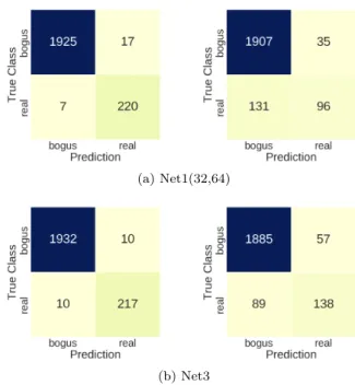
A meaningful evaluation measure (also for unbalanced data) are confusion matrices containing both the number of cor-rectly classified instances as well as the number of misclassifi-cations. The confusion matrices for various models, obtained via the test set, are shown in Figure5. It can be seen that each method performs reasonably well, but some of the mod-els yield a significantly smaller number of misclassifications. In particular, one can make the following observations:
• Random Forest: The standard random forest performs reasonably well, which indicates that the features extracted from the difference images capture the main characteristics of the learning task. In total, 34 instances are misclassified out of all 2,169 instances, which corresponds to an MCC of 0.915. Note that a similar performance can be obtained by slightly different random forest models that stem from differ-ent splitting mechanisms or parameter assignmdiffer-ents (see Sec-tion3.2). However, none of these variants yielded an MCC better than 0.925.
• Shallow Networks: The conceptually very simple and shallow networks with only a single convolutional layer al-ready yield a surprisingly good performance that is com-petitive with the one of the random forest. The MCCs for the Net1(32,64), Net1(64,128), and Net1(128,256) are 0.937, 0.951 and 0.933, respectively. We will investigate these net-works and their classification performances in more detail below.
• Deeper Networks: The deeper networks with two or three convolutional layers yield a slightly better classifica-tion performance than the shallow networks. Applying data augmentation steps prior to training the networks seem to further reduce the number of misclassifications (see below). The MCC for Net2 and Net3 without any further data aug-mentation and transformation steps are 0.949 and 0.954, re-spectively. Net3 only misclassifies 21 out of the 2,169 in-stances and, hence, 13 less than the random forest (in par-ticular, it misses less “real” sources that are assigned to the “bogus” class).
It is worth mentioning that the classification perfor-mance is, in general, very similar for slightly different con-volutional neural networks, i. e., neither the particular net-work structure nor the involved parameters seem to have a significant influence on the final classification performance. The conclusion one can draw at this point is that standard “out-of-the-box” convolutional neural networks seem to be well-suited for the task at hand and that even relatively sim-ple networks yield a performance that is competitive with state-of-the-art approaches.
4.2.2 Shallow Networks
Although being conceptually very simple, the shallow net-works already yield a very good classification performance. This is actually surprising since the images are obtained un-der different observational conditions (such as the phases of the moon) that will lead to background levels that differ from image to image even though the same region/object is observed. Intuitively, “subtracting” this background level in the preprocessing phase should simplify the learning problem and is, for this reason, also part of other ap-proaches (Brink et al. 2013). However, we observed that such a normalisation step in the preprocessing phase actually de-creases the classification performances of the networks, both for the shallow and deeper models.
To investigate why the shallow networks already perform so well, we consider the simplest architecture, Net1(32,64), which only contains a single convolutional layer. In Figure 6, the activations of the feature maps in-duced by a “bogus” and a “real” instance are shown. In both instances, there appears to be feature maps that activate on
(a) Random Forest (b) Net1(32,64) (c) Net1(64,128) (d) Net1(128,256) (e) Net2 (f) Net3 Figure 5. Confusion matrices for each of the considered models. While the random forest already achieves a good classification perfor-mance, the different networks, also the simple ones, seem to yield competitive or even slightly better results.
(a) “bogus” (b) “real”
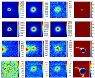
Figure 6. Activations (feature maps) of the convolutional layer of Net1(32,64) given a “bogus” and “real” source, respectively. The top row shows the three input images that are available for each instance. Below the red line, the 32 feature maps are provided that are induced by the convolutional layer of Net1(32,64).
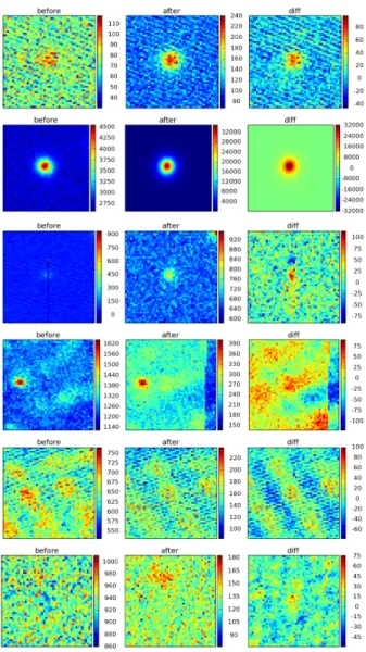
the background (“dark centre”), while other maps activate on different parts of the centre. This suggests that the net-work can distinguish between the source itself and the back-ground, thus being able to classify images relatively unhin-dered by different levels of noise. We also consider occlusion maps (Zeiler & Fergus 2014) for Net1(32,64). To determine if a certain area of an image is important for the classification, one can mask this area and see how this affects the predic-tion of the model. In Figure7, occlusion maps are shown for several “real” and “bogus” instances. In these occlusion maps, the value of a pixel (x, y) represents the predicted probability of the correct class by the model, after all pixels in a 3 × 3 square centred on pixel (x, y) have been set to zero. Using the occlusion maps, one can gain insight into the way the model makes its predictions. For the “real” sources, occluding pixels in the centre of an image causes misclassifications, while oc-cluding the edges of the image has little to no effect. This is a good sign, as any other behaviour could indicate a reliance on artefacts or patterns in other regions of the image than the center. For the “bogus” instances, occluding any part of the image often makes little to no difference in classification. This indicates that the network learns that the absence of a source is an indicator for “bogus” and as such, obscuring the “bogus” source will still result in a correct classification.
In summary, as expected, the shallow networks seem to
Figure 7. Input images along with occlusion maps (right col-umn) for two “bogus” (top) and two “real” (bottom) sources. The different colours along with the colour bars illustrate the pixel intensities for each of the three left images per row, whereas they sketch the different probabilities for the occlusion map in the rightmost image per row. For the “real” sources, the centres of the input images seem to be important, whereas for the “bogus” instances, obscuring any part of the image appears to have little effect.
mainly focus on the centre (e. g., “is there anything in the centre in the target image”).
4.2.3 Data Augmentation
One of the main challenges that needs to be addressed is the shift from the given training data to completely new, unseen objects. Since the number of “real” sources is very small (e. g., only very few distinct supernovae objects are known and, hence, available for training), one has to develop a system that cannot only detect similar objects, but also new “real” sources whose image representation is related, but different (e. g., a rotated version of an image contain-ing a star, supernova, or artefact). A simple yet effective approach to improve the generalisation performance of con-volutional neural networks is to augment the training data, see Section3.3for details and the particular augmentation steps conducted. Note that we only apply the augmentation on the training, the test set is not modified.
The results for the deeper networks, Net2 and Net3, enhanced with the data augmentation steps are shown in Figure8. Given that we increase the number of instances in
(a) Net2 (b) Net3
Figure 8. Confusion matrices for Net2 and Net3 with data aug-mentation steps conducted in the preprocessing phase.
the training data with augmentation, we also increase the number of training iterations from 1,000 to 5,000. The con-fusion matrices in Figure8show that the addition of a data augmentation step can further improve the classification per-formance with Net3 only causing 14 overall misclassifications for the test dataset. We expect further data augmentations steps to be helpful as well in this context, see Section5.
4.2.4 Analysis of Misclassifications
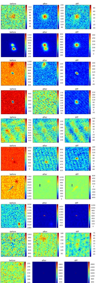
Both Net2 and Net3 only misclassify a small number of test instances. In Figures 9 and 10, all misclassifications made by Net3 (with data augmentation) are shown. For the first type of error, “bogus” objects misclassified as “real”, com-mon examples are due to non-uniform background noise in the template and/or target images, or deficits in the tem-plate image that, after convolution, resemble point sources in the difference image. For the other type of error, “real” instances misclassified as “bogus”, a single object (with mul-tiple observations) is misclassified (top six images). This is very reasonable since it is generally very hard for any model to distinguish varying stars and multiple follow-up observa-tions of a new supernova. However, from a practical per-spective, such cases can easily be handled by flagging such a source as “real” the first time it is observed (and correctly classified as “real”). The remaining two (last two rows) de-pict a low signal-to-noise detection of a faint supernova near the core of its host galaxy, and an asteroid moving quickly enough to show a trail in the target image.
The two deeper convolutional neural networks yield sig-nificantly less misclassifications as the baseline random for-est approach (see the appendix for some misclassifications made by the random forest). Interestingly, the misclassifi-cations differ slightly, i. e., the ones of Net3 do not form a subset of those misclassified by the random forest. We will see that this can actually be beneficial when combining the different classifiers.
4.2.5 Less Input
The networks considered so far are trained on all three input images that are available for each instance. By providing all the data, the networks can automatically determine which input images are important (see discussion above concerning the weights). A natural question is whether a competitive performance can also be achieved using less input data. We consider two settings: (1) Using only the template and target
Figure 9. Misclassifications made by Net3 with data augmen-tation (“bogus” instances misclassified as “real”). The different colours along with the colour bars illustrate the pixel intensities per image.
images and (2) using only the difference image. Note that the latter setting usually forms the basis for other techniques that extract features from the difference images only.
We focus on the simplest network considered in this work, Net1(32,64), and the best-performing one, Net3 with data augmentation. The induced confusion matrices are shown in Figure11. By comparing this figure to Figure 5, it can be seen that using only template and target images yields a competitive performance compared to using all three input images. This may seem surprising due to the majority of the existing schemes being based on difference imaging. The results, however, clearly indicate that the reduced set of input images is sufficient for approaching the task at hand. This depicts a desirable outcome since one might be able to omit image subtraction steps in future detection pipelines. Further, the networks trained using only the difference im-ages yield a significantly worse classification performance. Hence, using only this type of information seems to be not enough for convolutional neural networks in this context.
Figure 10. Misclassifications made by Net3 with data augmen-tation (“real” instances misclassified as “bogus”). The different colours along with the colour bars illustrate the pixel intensities per image.
4.2.6 Ensembles
A common way to improve the classification performance is to consider ensembles of different models. As mentioned above, random forests depict ensembles of classification or regression trees and usually yield a significantly better
per-(a) Net1(32,64)
(b) Net3
Figure 11. Classification performance of Net1(32,64) and Net3 (with data augmentation) in case only the template and target (left) or the difference images (right) are provided to the networks.
(a) E1 (b) E2
Figure 12. Confusion matrices for two ensemble classifiers. E1 combines three different neural networks. E2 two neural networks and a random forest.
formance than the individual models. We consider two en-sembles E1 and E2:
• E1: Net2 (data augmentation), Net3 (data augmenta-tion), Net1(32,64) (template and target images only), and Net3 (data augmentation, template and target images only). • E2: Net2 (data augmentation), Net3 (data augmenta-tion), and the random forest model.
The results are shown in Figure12. It can be seen that en-sembling reduce the number of misclassifications. Further-more, incorporating the random forest appears to be benefi-cial, potentially due to features that capture the character-istics of special cases.
The improvements over the best-performing single con-volutional neural networks are really small and, due to the relatively small test dataset, we do not argue that the en-sembles outperform the individual classifiers. Nevertheless, the ensembles might exhibit a slightly better performance on completely new, unseen data since the combination of many different classifiers usually yield more “stable” results.
4.2.7 Receiver Operating Characteristic (ROC) Analysis All results reported so far are based on the default threshold of 0.5 for deciding which class an instance should belong to given the probability scores. For random forests, this simply corresponds to a majority vote among the individual trees. For the convolutional neural networks, it means the class with the highest probability. In general, many more “bogus” than “real” instances are observed in practice and one might want to adapt the choice for the threshold. For example, one might prefer finding more “real” sources at the cost of an in-crease in false positives (i. e., “bogus” instances misclassified as “real”). This naturally depends on the number of human experts being available for manual inspection of all instances classified as “real” sources by the model.
To quantify the performance of a model across a range of thresholds, one can make use of so-called receiver operating characteristic (ROC) curves (Fawcett 2006). Here, the recall t p · (t p+ f n)−1 = tp · P−1 is also called true positive rate (TPR), where P denotes the number of all positive (“real”) instances. Accordingly, one can define the false positive rate (FPR) as f p · ( f p+ tn)−1 = f p · N−1, where N corresponds to all negative (“bogus”) objects. A classifier assigning only the class “real” to all instances would therefore achieve an optimal TPR of 1.0, but also a potentially very large FPR. Ideally, one would like to have a large TPR and a small FPR; a ROC curve captures this trade-off.
In Figure 13 the ROC curves for various models are shown. Of the models plotted, Net3 has the best perfor-mance, which we can verify by calculating the area under the ROC curve (AUC). The AUC values for the models are given in Table3. To test the significance of the differences in AUC values, we apply two statistical tests for ROC curves: the so-called DeLong (DeLong et al. 1988) and the boot-strap (Hanley & McNeil 1983) methods. In both cases, we test the null hypothesis that the performance of both models is the same against the alternative hypothesis that Net3 per-forms better than the random forest (one-sided test). This results in p-values of 0.0359 and 0.0352, respectively, indi-cating that Net3 has a significantly better performance than the state-of-the-art random forest approach. Even though this improvement seems small, it could result in a large de-crease in false positives due to the large number of transient candidates that are generated each night.
The confusion matrix for NET1(32,64) shows that we have a TPR of 0.956 for the standard threshold of 0.5. By moving right on the ROC curve, both the TPR and FPR increase and the decision of which FPR is still deemed ac-ceptable is up to the user. In the case of transient vetting, the optimal threshold is determined by the capability to do follow-up studies on the possible transients and the will-ingness to search through a lot of extra “bogus” candidates to find a couple more transients. Such decisions have to be made per project and based on the human resources that are available to manually check the output of the processing pipelines.
5 CONCLUSIONS AND OUTLOOK
We propose deep convolutional neural networks for the task of detecting astrophysical transients in future all-sky survey
Table 3. AUC for the different models.
Model AUC
Random forest 0.9907 Net1(32,64) 0.9914
Net3 0.9972
E2 0.9946
Figure 13. ROC curves for various models. The individual per-formances for a threshold of 0.5 are marked for each curve.
telescopes. The currently used state-of-the-art approach is based on feature extraction and a subsequent application of random forest algorithms. In our experimental evalua-tion, we demonstrate that even conceptually simple net-works yield a competitive performance, which can be im-proved further via deeper architectures, data augmentation steps, and ensembling techniques. It is also worth mention-ing that the networks considered also perform well (or even better) by just using template and target images, i.e., the networks do not rely on image subtraction. This might pave the way for future classification pipelines not containing im-age subtraction preprocessing steps.
The machine learning models proposed in this work can be adapted and extended in various ways. Future telescope projects will produce significantly more data and we expect that taking such additional training instances into account will be beneficial to further improve the classification perfor-mances. The detection of extremely rare objects or artefacts will always depict a problem (even with better models due to many more objects being considered per night). Appropri-ate data preprocessing and augmentation steps conducted in the training phase might be one way to handle such in-stances correctly. In addition, adapting deep convolutional neural networks to the specific needs of the tasks at hand might be essential to cope with upcoming learning scenarios in this field (e. g., by considering specific loss functions that are suitable for extremely unbalanced datasets). We plan to investigate such important and interesting extensions in the near future.
ACKNOWLEDGEMENTS
FG and VARMR acknowledge financial support from the Radboud Excellence Initiative. VARMR further acknowl-edges financial support from FCT in the form of an ex-ploratory project of reference IF/00498/2015, from CIDMA strategic project UID/MAT/04106/2013, and from Enabling Green E-science for the Square Kilometer Array Research Infrastructure (ENGAGE SKA), POCI-01-0145-FEDER-022217, funded by Programa Operacional Competitividade e Internacionaliza¸c˜ao (COMPETE 2020) and FCT, Portugal.
REFERENCES
Alard C., 2000,A&AS,144, 363
Alard C., Lupton R. H., 1998,ApJ,503, 325 Bertin E., Arnouts S., 1996, A&AS,117, 393
Bertin E., Mellier Y., Radovich M., Missonnier G., Didelon P., Morin B., 2002, in Bohlender D. A., Durand D., Handley T. H., eds, Astronomical Society of the Pacific Conference Se-ries Vol. 281, Astronomical Data Analysis Software and Sys-tems XI. p. 228
Bloom J. S., et al., 2012,PASP,124, 1175 Breiman L., 2001, Machine Learning, 45, 5
Brink H., Richards J. W., Poznanski D., Bloom J. S., Rice J., Negahban S., Wainwright M., 2013,Monthly Notices of the Royal Astronomical Society,435, 1047
Buisson du L., Sivanandam N., Bassett B. A., Smith M., 2015, MNRAS,454, 2026
Charnock T., Moss A., 2016, preprint, (arXiv:1606.07442) Coates A., Huval B., Wang T., Wu D. J., Catanzaro B. C., Ng
A. Y., 2013, in Proceedings of the 30th International Confer-ence on Machine Learning (ICML). JMLR.org, pp 1337–1345 DeLong E. R., DeLong D. M., Clarke-Pearson D. L., 1988,
Bio-metrics, pp 837–845
Dieleman S., et al., 2015a, Lasagne: First release., doi:10.5281/zenodo.27878, http://dx.doi.org/10.5281/ zenodo.27878
Dieleman S., Willett K. W., Dambre J., 2015b, Monthly Notices of the Royal Astronomical Society, 450, 1441
Fawcett T., 2006, Pattern Recognition Letters, 27, 861
Geurts P., Ernst D., Wehenkel L., 2006, Machine Learning, 63, 3 Glorot X., Bengio Y., 2010, in Proceedings of the Thirteenth In-ternational Conference on Artificial Intelligence and Statistics AISTATS. pp 249–256
Goldstein D. A., et al., 2015,AJ,150, 82
Hanley J. A., McNeil B. J., 1983, Radiology, 148, 839
Hastie T., Tibshirani R., Friedman J., 2009, The Elements of Statistical Learning. Springer
Ivezic Z., et al., 2008, preprint, (arXiv:0805.2366)
Kaiser N., et al., 2010, in Ground-based and Airborne Telescopes III. p. 77330E,doi:10.1117/12.859188
Keller S. C., et al., 2007,Publ. Astron. Soc. Australia,24, 1 Kim E. J., Brunner R. J., 2016, preprint, (arXiv:1608.04369) Kingma D. P., Ba J., 2014, CoRR, abs/1412.6980
LeCun Y., Boser B., Denker J. S., Henderson D., Howard R. E., Hubbard W., Jackel L. D., 1989, Neural Computation, 1, 541 LeCun Y., Bengio Y., Hinton G., 2015, Nature, 521, 436 Matthews B. W., 1975, Biochimica et Biophysica Acta, 405, 442 Morii M., et al., 2016, preprint, (arXiv:1609.03249)
Murphy K. P., 2012, Machine Learning: A Probabilistic Perspec-tive. The MIT Press
Nissanke S., Kasliwal M., Georgieva A., 2013,ApJ,767, 124 Nouri D., 2014, nolearn: scikit-learn compatible neural network
library.https://github.com/dnouri/nolearn
Pedregosa F., et al., 2011, Journal of Machine Learning Research, 12, 2825
Perlmutter S., et al., 1999,ApJ,517, 565 Rau A., et al., 2009,PASP,121, 1334 Riess A. G., et al., 1998,AJ,116, 1009
Scalzo R., et al., 2017, preprint, (arXiv:1702.05585) Schmidt B. P., et al., 1998,ApJ,507, 46
Smartt S. J., et al., 2016,MNRAS,462, 4094
Theano Development Team 2016, arXiv e-prints, abs/1605.02688 Wright D. E., et al., 2015,MNRAS,449, 451
Zeiler M. D., Fergus R., 2014, in European Conference on Com-puter Vision. pp 818–833
APPENDIX A: MISCLASSIFICATIONS
FiguresA1andA2show misclassifications made by the ran-dom forest baseline. All false positives instances are given in Figure A1, whereas only a subset is given for the false negatives in FigureA2.
This paper has been typeset from a TEX/LATEX file prepared by the author.
Figure A1. A subset of the “bogus” objects misclassified as “real” by the random forest model. The different colours along with the colour bars illustrate the pixel intensities per image.
Figure A2. A subset of the “real” objects misclassified as “bogus” by the random forest model. The different colours along with the colour bars illustrate the pixel intensities per image.