Pairs Trading: Strategy
Refinements
Trabalho Final na modalidade de Dissertação apresentado à Universidade Católica Portuguesa
para obtenção do grau de mestre em Finanças
por
Ricardo Jorge Madureira Ribeiro
sob orientação deProf. Doutor Paulo Alves Dr. João Novais
Universidade Católica Portuguesa abril de 2015
Acknowledgments
I would like to thank my father, my mother and my sister for giving me the opportunity to realize this master, for having supported me in every step of my life and I am grateful for that every day.
I also thank my girlfriend for the help, the patience and all the love shown during all this time, this thesis would not be the same without you.
I would like to express my deepest appreciation to Prof. Doutor Paulo Alves and Dr. João Novais for the help, the guidance and all the advices given during this period.
A big thanks to Prof. Doutor Ricardo Ribeiro for the help with the statistical platforms.
Last but not least, I want to express my gratitude to Prof. Doutor Ricardo Cunha for providing us a master with an excellent quality.
Abstract
In this paper, we apply the pairs trading strategy, original presented by Nunzio Tartaglia in mid-80´s, for the period between 2004 and 2014, to stocks listed in the London Stock Exchange. Our trading strategy seems to be highly profitable, with an average 6-month excess return of 15.39%. The strategy also proved to have better results when faced trouble economic environments like the subprime crisis.
We have implemented several add-ons to the strategy, aiming to reduce its risk. A new liquidity restriction was implemented in selecting pairs so that the strategy is not constrained by any concerns about liquidity problems. Another implementation was the creation of stop loss strategies based on number of days with losses and by loss percentage, which, however, proved to be unrewarding on the attempt to maximize the returns. On the other hand, by proving the unfeasibility of the stop loss strategies, we also proved the robustness of our strategy because we perceive that even if the return of the pair is going down for consecutive days or for a certain percentage, it ends up converging.
Keywords: Pairs trading; Relative-value strategy; Refinements; Stop loss strategy;
Table of contents
1. Introduction ... 1
1.1 Requirements for the implementation of the strategy ... 3
2. Literature Review ... 6
3. Methodology ... 15
3.1 The beginning of the strategy ... 15
3.2 Creation of pairs ... 16
3.3 Closeness measure ... 17
3.4 Trigger moment and decision on what position to take ... 19
3.5 Excess return of a position ... 21
3.6 Limitations of the strategy (in general) ... 21
3.7 Refinements ... 23
3.7.1 Specific liquidity ... 23
3.7.2 Introducing bid and ask prices ... 25
3.7.3 Stop loss strategies ... 26
4. Results ... 27
4.1 Unconditional strategy compared to specific liquidity strategy ... 27
4.2 Profit/Losses: Where are they coming from? ... 30
4.3 Specific liquidity restriction strategy and introduction of stop losses ... 35
4.4 Detailed results of the strategies ... 38
4.5 Pairs trading: market neutral strategy or correlation to the market? ... 40
5. Conclusion and future work ... 42
List of figures
Figure 1: Example of pair formation and trading ... 16
Figure 2: Example of the creation of pairs with 4 firms ... 17
Figure 3: Normalized returns of a pair in the formation period... 18
Figure 4: Trading period of a pair ... 20
Figure 5: Number of pairs in each trading period ... 24
List of tables
Table 1: Sample per industry ... 15 Table 2: Results of both strategies using the top 20 pairs without any restriction. ... 28
Table 3: Results of both strategies using the limited pairs by specific liquidity restriction. ... 28
Table 4: Detailed results of limited pairs strategy ... 31 Table 5: Detailed results of trades (of the limited pairs strategy) that went positive and negative and closed before the last day and in the last day. ... 34
Table 6: Results of the limited pairs’ strategy with the bid and ask prices and with the inclusion of 4 different stop loss strategies ... 36
Introduction
Over the last years, many strategies have been developed by financial and banking institutions in order to obtain steady profits while, at the same time, attempt to decrease their risk. Pairs trading is an example of such developments, attributed to Nunzio Tartaglia while working at Morgan Stanley. Tartaglia joined a team of mathematicians, physicists and computer scientists, and tried to develop quantitative arbitrage strategies with automated trading systems which, at that time, was something really innovator (Vidyamurthy, 2004). Tartaglia and his group started to apply their new strategy in 1987 and many other started to follow and soon it became a common strategy for hedge funds (Gatev et al., 2006) and financial institutions, but has yet to catch the interest of academics.
The base for the strategy is the identification of trading pairs – a set of two stocks (or any other financial instrument) that we will track during certain period of time and, if certain criteria are met, traded on. For two stocks to be considered as a trading pair, they must satisfy two conditions: i) have similar daily price patterns over a certain period; and ii) be exposed to similar systematic risk during the trading period1. However, we can mitigate part of the risk that arises from the non-systematic risk, which is the risk that is intrinsic to a firm or sector, by choosing pairs arbitrarily, without taking into account their specific sector.
We can use a metaphor to give an overview about pairs trading, presented by Whistler (2004). Let’s imagine a motorway and a service road which are parallel between each other. The service road will follow the motorway really
1 The systematic risk is a type of risk that derives from macroeconomic factors (Bodie, Kane, & Marcus, 2013).
closely, except when a terrain, a house or other obstacle appears in the middle of the two roads. But, after that obstacle, the motorway and a service road will converge and will be close again.
One can describe the pairs trading strategy as follows. All pairs of stocks are followed over one year (formation period) and those ones with very high price changes correlation will be selected. Then, the selected pairs will be tracked during 6 months (trading period) and a trading position is open in both stocks (short in the stock with relatively higher normalized prices and long in the stock with relatively lower normalized prices) when the normalized prices of the stocks diverge above a certain level. Based on historical statistical correlation, the strategy assumes that normalized prices will very likely converge. The larger the spread, the greater the potential profits. Finally, a position is closed when the normalized prices of the stocks converge and “cross” or when we reached the end of the trading period.
Hereupon, we can assume that we are selling the “overvalued” securities and buying the “undervalued” securities and, in that sense, trying to profit from future prices adjustments, which makes pairs trading a relative-value investment strategy. However, it’s not easy to determine if the price is over or undervalued because, in order to do that, we need to know the true value of the security in absolute terms, which is not an easy achievement. The pairs trading strategy overcomes this problem by using the relative pricing (that’s why it is called a relative-value investment strategy). If two securities are similar, have similar characteristics and an identical behaviour, we assume that their prices changes must be the same or, at least, similar. As Vidyamurthy (2004) states, for our strategy “the specific price of the security is not important. (…) it is only important that the prices of the two securities be the same”. On the other hand, Tartaglia puts the psychological aspect as an explanation of pairs trading saying
that “… human beings don’t like to trade against human nature, which wants to buy stocks after they go up not down.” (Hansell, 1989).
Throughout our study, it will also be important to understand how pairs trading strategy reacted in a troubled economic environment, which is embedded in our study by including the subprime crisis that was developed in United Kingdom between 2007 and 2009 (www.bloomberg.com). When the peak occurred, United Kingdom government intervened with actions as the “bank rescue package” (action taken due to severe fall of the stock exchange and due to a huge concern about the stability of the British banks) and the “Bonus Supertax” (tax for banker’s bonuses to avoid the risk of new crisis in banking sector). Therefore, it would be relevant to see the reaction of pairs trading returns in these specific years.
1.1 Requirements for the implementation of the strategy
In order to implement the strategy, a market inefficiency must be present (an imbalance). The point is to detect that inefficiency and, consequently, obtain profit until the moment the market agents realize that this inefficiency exists and correct it.As said above, our best pairs are the ones that have a similar systematic risk and also close variations between themselves. Considering this, they should also have a high price movement correlation over time, meaning that we should not find large differences in price movements. Assuming that no shock happens2 and that the two pairs meet the two conditions presented before, we can assume that we have a risk-free portfolio. In other words, this means that if we take a long position in one stock of the pair and a short position on the other stock of the same pair, we would have a portfolio without any excess return
2 This is valid only if no idiosyncratic shock occurs. In the presence of such a shock, for instance the release of
and also without any risk. This happens because when one stock goes up, the other one will follow this increase, otherwise, the law of one price (from now on called LOP) and their conditions would be broken.
The LOP is a concept based on several conditions but, in general, states that a stock must have the same price in different markets, already including the exchange rates and the transaction costs. Otherwise, an arbitrage opportunity will exist simply from buying the stock with the lower price in one concrete market, and selling that same stock, but in other market where it has a higher price.
One of the conditions of the LOP states that if two financial instruments have the same value and risk drivers, the relative price of the two should result in a stable relationship (again, if no idiosyncratic shock happens). If this condition is not met, we have an arbitrage opportunity that should be exploited. This rationale was the backbone of Gatev, Goetzmann, & Rouwenhorst (2006). They based their study on violations of the LOP, exploiting situations where the price between the two stocks of the pair differed more than two historical standard deviations. Later, we will develop the results obtained in their research and our view about it, nonetheless, by looking at this simple explanation, we can see that the strategy followed exactly the situations that the LOP predicts. Gatev et al. (2006) followed the pairs for one year, and then analysed them by measuring the closeness between the two stocks. After that year, if no idiosyncratic shock happens, the prices of the two stocks should still have a stable relation. Therefore, Gatev et al. (2006) looked at the daily price of the two stocks and if the difference between the two became larger than two historical standard deviations, they went short on the winner (in this case, the stock that went up) and went long on the loser (in this case, the stock that went down). The reason for doing this is due to the fact that, in the future, the gap that exists between this two stocks will probably become null, this is, the price will converge to
meet the principle of the LOP above mentioned. Let’s imagine that the price of the stock that previously went up, now goes down, converge and “cross” the price of the stock that previously went down and that now, for this purpose, remained the same. As Gatev et al. (2006) had short the stock that went up, this convergence will generate a positive excess return.
Another characteristic of pairs trading, stated by Gatev et al. (2006), is that it is a market neutral strategy. Market neutral strategies, according to Vidyamurthy (2004), “are strategies that are neutral to market returns, that is, the return from the strategy is uncorrelated with the market return.” However, Gatev et al. (2006), also stated that “pairs trading might simply be more profitable in times when the stock market performs poorly.”
2. Literature Review
As pointed out above, pairs trading strategy nowadays is used by hedge funds and financial institutions but there is not a lot of researches developed by the academic community.
There are two studies that, because of their importance, marked pairs trading strategy academic literature. The first one, called “Pairs Trading: Performance of a Relative-Value Arbitrage Rule” (Gatev et al., 2006) and the second one, called “Pairs Trading and Accounting Information” (Papadakis & Wysocki, 2007).
Gatev et al. (2006) were the firsts to introduce pairs trading strategy academically, as we presented before. The implementation of pairs trading in their study has two stages. The first, being the formation period (12months) that represents the period of formation of pairs, and the trading period (6 months) that represents the period where they trade the pairs that were formed before. Besides, Papadakis & Wysocki (2007) followed this method, as we will also do. To form the pairs, Gatev et al. (2006) downloaded all the US stocks from CRSP daily files since 1962 until 2002, dropping the ones that had, at least, one day with no trade to ensure that in their sample they only had liquid stocks and, at the same time, this served to reduce the list of stocks and, consequently, simplify the pairs’ formation. Papadakis & Wysocki (2007) followed the same method (changing only the dates to 1981-2006), however, as we said before, we decided to use the London Stock Exchange. As also said, we chose the period between January of 2004 and June of 2014.
Thereafter, Gatev et al. (2006) formed the pairs by combining, in pairs, all the stocks without any restriction and using the normalized returns (including reinvested dividends) in order to compute the closeness variable. We decided to
follow their method, despite the fact that, Papadakis & Wysocki (2007) had changed the way to compute the pairs.
In Papadakis & Wysocki (2007) research they split the stocks in quintiles based in their 12-month stock return on the formation period. After, inside of each quintile, they split again the stocks in quintiles based on their 6-month return of the first half of the formation period. Finally, it was by using this method that they reached what they intended. They achieved 25 groups of stocks (each quintile of the first 5 quintiles created unfolds to new 5 quintiles, so they had 5x5=25 groups of stocks) that had similar profiles, this is, “the same co-movement over the 6-month and the 12-month horizons” (Papadakis & Wysocki (2007)). This appears to be harder and time consuming when compared to only creating a combination of all the pairs like Gatev et al. (2006) did, but, on the other hand, it can save some time afterwards, when it’s needed to compute the closeness measure.
The closeness variable was computed as the sum of the squared daily differences between the returns of each stock in the pair. By sorting them from the lowest to the highest, they had the closeness measure of all the pairs. Afterwards, Gatev et al. (2006) looked at the top 5, top 20 and top 20 after top 100 (101-120) and started trading after the last day of the formation period (thus beginning the trading period).
Gatev et al. (2006) started to trade in the beginning of every month in the sample period (except, of course, the first 12 months that were used to create the pairs). However, they used the close price of the stocks to compute the losses/gains in the trading period. This could be an almost irrelevant problem when considering stocks that have high liquidity and, consequently, also have a low bid-ask spread. Having a low bid-ask spread means that the bid and the ask price are near to each other, which implies that they are near to the close price, meaning that supply and demand are almost synchronized. Conversely
for stocks that, for some reason, do not have high liquidity this could be an issue of greater importance. Once they used the close price to enter into a long/short position in these stocks, they didn’t take into account the gap that existed between the bid and ask prices.
This could lead to some problems in Gatev et al. (2006) study because the average excess return presented by them at the first instance would be biased upward. What this means is that, implicitly, when they decided to use the price, they were using an approach to bid quotes when they bought the stocks that had performed bad, and an approach to ask quotes when they sold the stocks that had performed good.
Nevertheless, they recognized this issue. In order to avoid it, they “initiate positions in each pair on the day following the divergence and liquidate on the day following the crossing” (Gatev et al., 2006). However, by doing this, it functions like the example of a short blanket, simply meaning that if you try to cover your shoulders, you uncover your feet and if you try to cover your feet, you uncover your shoulders. This means that when they decided to wait one day to open the position after the pairs diverge more than two historical standard deviations, and to close the position after they converge and “cross”, they were not acting according to the strategy that they studied and initially presented. In practice this means that they were delaying the opening and the closing of the position in almost two days because they used the close price of the day after the “cross”.
Up to this point, Papadakis & Wysocki (2007) used the exact same strategy to compute their first results, which they eventually called “unconditional pairs trading strategy” (from Gatev et al. 2006), and, therefore, they had the same problem with the daily prices. Although they followed the same strategy, Papadakis & Wysocki (2007) presented a formula to the strategy to track the pairs’ position over the trading period (this formula was first presented by
Andrade et al. in their study in 2005). This may not be considered an improvement, however, it can be useful to understand which three positions our strategy can take. So, in order to make it easier to understand, they used a tri-state indicator variable, the "𝐼𝑡𝐴𝐵"as they called:
(1)
𝐼𝑡𝐴𝐵 ≡
0 𝑛𝑜𝑡 𝑜𝑝𝑒𝑛 +1 𝑠ℎ𝑜𝑟𝑡 𝐴; 𝑙𝑜𝑛𝑔 𝐵 −1 𝑙𝑜𝑛𝑔 𝐴; 𝑠ℎ𝑜𝑟𝑡 𝐵
This indicator serves to show what position we should take when a pair is open. A and B represent two stocks of one pair. +1 means that stock A has been outperforming stock B. -1 means the opposite, that stock B has been outperforming stock A. 0 means that the prices didn’t diverge more than two historical standard deviations. This indicator is of great importance because it helps us on tracking the stocks along the trading period using only three stages. This will be the methodology that we will follow in our work, in order to find the position that we have to take in each stock and this choice was made in order to simplify the trade.
As we said before, until this moment, Papadakis & Wysocki (2007) followed the exact same strategy to compute their first results, however, at this stage, we already added two new improvements to the strategy. One of them serves to avoid the close daily price problem. This means that daily prices will not be a problem in our study because we will use ask and bid prices to our strategy (to buy and sell, respectively), thus, we will not have to delay our entrance in the market. Under these circumstances we don’t have to deal with data biased by bid-ask bounce. We can now follow the strategy studied and enter into the market on the day the pairs actually diverge, and exit the market on the day the pairs converge. The other improvement we already introduced was the specific liquidity measure. We will address this topic later (section 3.7.1), though we can
already say that we introduced this new restriction to reduce some liquidity problems of the strategy.
First, we will look at the results achieved by Gatev et al. (2006). For the unrestricted stocks (stocks that were not paired by industry, sector or other restriction) in the simple strategy, without waiting one day to open and to close positions (the biased strategy), they found an average excess monthly return of 1.31% for the top 5 pairs, 1.44% for the top 20 pairs and 1.08% for the top 101-120 pairs. On the other hand, after adding the rule of “one day waiting” (as we explained before, open/close a position one day after the pairs diverge and converge respectively), the profits from this strategy dropped to 0.75% for the top 5 pairs, 0.895% for the top 20 pairs and 0.795% for the top 101-120 pairs.
Gatev et al. (2006) also computed some trading statistics that were relevant to compare afterwards with our own results. On the top 5 pairs, they found that, on average, 4.81 pairs open a position during the trading period and that the average number of round-trips per pair was 2.02. In other words, in a trading period, normally, a pair performs about 2.02 complete trades (by complete we mean a trade that opens and closes). Also, the average duration of an open position is 3.75 months. They also tested pairs trading in separated sectors but concluded that it was profitable in all of them and not only limited to one or a few sectors.
On their study, they detected that pairs trading “performed well over difficult times for U.S. Stocks.” (Gatev et al. 2006). They found that when the U.S. stock market had a decline, pairs trading strategy performed better than in any other period. On the other hand, when the U.S. stock market had his best years during the sample period (mid-1990s), pairs trading strategy had almost insignificant profits. With this evidences, they suggested that “pairs trading might simply be more profitable in times when the stock market performs poorly.”(Gatev et al. 2006). This is a crucial point for our study. As we already
introduced before, our strategy was realized in a particular economic environment that includes the subprime crisis. It will be interesting to see how pairs trading performed in this particular years and see if their statement was accurate. To summarize, Gatev et al. (2006) applied this strategy from 1962 until 2002 and had an average annualized excess returns of about 11% for self-financing portfolios of pairs. Also, one of the main conclusions is that the robustness of the excess returns suggests that the profit of the pairs trading strategy comes from the temporary mispricing of close substitutes.
We should now consider the results presented by Papadakis & Wysocki (2007). They started to compute the results by applying the same exact strategy that Gatev et al. (2006) had presented a year before but using their own study years (1981-2006). They found an average monthly excess return of 0.62%. Comparing to the study of Gatev et al. (2006) (0.895%) the profitability is lower and that’s justified by the authors with the inclusion of more recent periods in their analyses. The position was normally open when the price diverged more than 5.47% and the average time that a pair remained open was 3.6 months, while the average number of pairs that were traded during the trading period was 19 (on the top 20).
After matching their strategy with the one created by Gatev et al. (2006), they searched for improvements that could be added to the first strategy and, for that reason, they looked for the impact of accounting information events (earnings announcements and analysts’ earnings forecasts) on the profitability of the strategy. Hereupon, they checked the profitability of pairs that opened after a) an earnings announcement and b) a clustered analyst forecasts. For the first one (a)), they recognized that pairs that opened after an earnings announcement represented 9% of all the trades of a period (trading period) and the average monthly excess return of these pairs was 0.07% (statistically insignificant) compared to the 0.62% of the unconditional method. This means
that they concluded that pairs that opened in a short period after earnings announcements were unprofitable.
For the second one (b)), they found that pairs that opened after a clustered analyst forecasts represented 14% of all the trades of the period (19% if we look at the period between 1994 and 2006, which can be justified by the increase of analysts activity and also clustered analyst forecast on this period). The average monthly excess return for this type of positions was -0.12%, again, compared to the 0.62% of the unconditional method. Lastly, they assumed that pairs that opened in a short period after a clustered analyst forecast event were unprofitable and “the relative drift in individual prices offsets the potential for convergence in the stock prices of the pair firms” (Papadakis & Wysocki, 2007).
After achieving these results, they searched for the trades that closed in those same situations (after an earnings announcement and after a clustered analyst forecast revision), and tried to find ways where they could have more profit, knowing now that the stock prices suffer some drifts when a significant accounting event happens. They tried to delay the close of the position after a significant accounting event took place, even if the prices of the stocks in the pair crossed. The justification for this option comes from the accounting events, meaning that they assumed that the cross had happened because the drift of the prices was due to the accounting event that occurred. By delaying the close of the position, they are changing the strategy proposed by Gatev et al. (2006). This new strategy will generate higher profits if:
After the cross, the price of the stock they went short keeps falling;
After the cross, the price of the stock they went long keeps rising;
Both situations mentioned above occur.
Thus, after the cross, they kept tracking the performance of the pairs after 5, 10 and 15 trading days (corresponding to 1, 2 and 3 weeks of trade), excluding only the cases where the close of the position matched with the end of the
trading period. Through implementing this type of strategy, they proved that the strategy could be improved in 0.08%, 0.17% and 0.22% by delaying the close of the position in 5, 10 and 15 days, correspondingly. They also explored for the profit they could get by delaying the close of the position in non-event periods and concluded that there were no gains, compared to Gatev et al. (2006) strategy, and this indicates a “concentration of drift around accounting related events.” (Papadakis & Wysocki, 2007).
They also applied the exact same strategy after a clustered analyst forecast revision event occurred. Compared to Gatev et al. (2006), they got an increase of 0.02%, 0.15% and 0.31% by delaying the close of the position in 5, 10 and 15 trading days, respectively. Hereupon, we can conclude that we can get an increase on the profits by delaying the close of the position if an earnings announcement event or a clustered analyst forecast revision event occurs.
Do & Faff (2010) performed a study in order to detect if pairs trading strategy (using US stocks) was still profitable after adding trading costs, like commissions and short-selling fees, in the period between 1963 and 2011. Accordingly, after all these costs were added to the strategy, pairs trading proved to be profitable in this period but in no way can be compared to the high profitability found in Gatev et al. (2006) research. They also concluded that this strategy has better returns in periods of crisis, like the global financial crisis in the late-2000s. Part of our study includes this timeline, and that will be crucial in order to compare these results with the ones that we obtained in this period of crisis.
Andrade et al. (2005) also applied one year before the strategy that was presented by Gatev et al. (2006), using the Taiwan Stock Exchange and achieved two conclusions. The first one was that the pairs trading strategy applied in this market, between the periods of 1994 to 2002, had an annual excess return of 10.18%. Furthermore, they found that “returns cannot be explained by exposure
to known sources of systematic risk.” (Andrade et al., 2005). Also, and even more important, they established that the profitability of pairs trading was linked to uninformed trading shocks, and, therefore, they also showed that “uninformed net buying is significantly correlated with a pair’s initial price divergence” (Andrade et al., 2005). Finally, they concluded that the pairs trading strategy had a low risk exposure because a position “is effectively hedged by an offsetting position with similar factor loadings” (Andrade et al., 2005).
3. Methodology
3.1 The beginning of the strategy
To implement the pairs trading strategy, we started by focusing our study on the London Stock Exchange. We chose this specific index because the most well-known studies were conducted with US stocks and we wanted to: a) extend the literature by studying other markets; and b) analyse if the results hold in a different institutional setting.
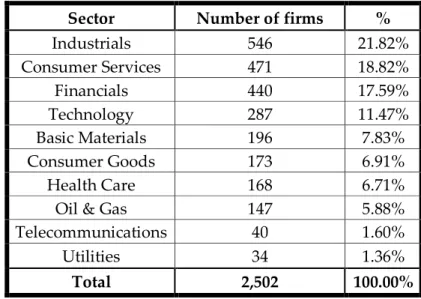
Our period of analysis started in the beginning of 2004 and ended in June, 2014. Afterwards, we will explain how we created the formation and trading periods. We retrieve our data from Datastream, creating a sample of all London Stock Exchange listed firms. We then dropped firms with total assets equals to zero or not available. This is a very quick way to filter inactive, delisted or suspended firm. Our final sample comprises 2,502 firms, as in Table 1 below:
Sector Number of firms %
Industrials 546 21.82% Consumer Services 471 18.82% Financials 440 17.59% Technology 287 11.47% Basic Materials 196 7.83% Consumer Goods 173 6.91% Health Care 168 6.71%
Oil & Gas 147 5.88%
Telecommunications 40 1.60%
Utilities 34 1.36%
Total 2,502 100.00%
3.2 Creation of pairs
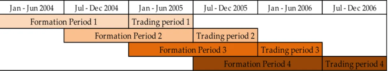
After the creation of our database, we started to create the pairs. We began a formation period in every 6 months. With this choice, and by not opting to do a formation period each calendar year, we will not have to wait 6 months every year to start a trading period and, therefore, we will have 19 trading periods instead of having just 10 trading periods. Below, in figure 2, it is possible to understand how did we created each formation and trading period:
Before we started to compute the possible pairs, we added one restriction. For every 6 months of our analysis, we dropped all the stocks that haven’t had, at least, 120 trading days on those 6 months. If a stock didn’t had more than 120 trading days in a 6-month window, it would be dropped out from all the formation periods in which it was inserted. For example, if a stock that during the 6-month window, comprehended between January of 2005 and June of 2005, didn’t trade for more than 120 days, it would be dropped out from two formation periods: the formation period that started in July of 2004 and that extended until June of 2005, and the formation period that started in January of 2005 and that extended until December of 2005. Once we know that the trading days can differ between 129 and 132 days, depending on the year, we will only have liquid stocks on our entire sample because we will never be trading a stock that in its formation period proved to be illiquid. We have then computed all the possible pairs, applying just one restriction, which was not to repeat
Jan - Jun 2004 Jul - Dec 2004 Jan - Jun 2005 Jul - Dec 2005 Jan - Jun 2006 Jul - Dec 2006 Trading period 1 Trading period 2 Trading period 3 Trading period 4 Formation Period 4 Formation Period 1 Formation Period 2 Formation Period 3
pairs that were already created (i.e., if we have the pair AB, we don’t want the pair BA). We can see below, on Figure 3, an example:
Mathematically, what we did was to create all the possible combinations without repeating any of them, by applying this formula:
(2) 𝑛!
𝑟! ∗ (𝑛 − 𝑟)!
where “n” represents the number of firms we have and “r” represents how many firms we want to combine at one time and, in pairs trading strategy, as the name already implies, “r” will always be equal to 2 because the goal is to find pairs.
3.3 Closeness measure
Afterwards, we followed the price through the formation period and we normalized the returns (including reinvested dividends) of this period to day 1. After having all the returns of this period for all the pairs, we computed the closeness measure. We did this by taking the normalized returns, subtracting one to the other, day by day, and squaring them and then, finally, summing all
Companies A B C D BD CD Pairs AB AC AD BC
these daily differences. Below, in Formula 2, is the mathematical description of this step: (3)
Closeness
𝑠𝑡𝑜𝑐𝑘 𝑎|𝑠𝑡𝑜𝑐𝑘 𝑏= ∑
(
𝑛 𝑖=1𝑃𝑎
i + 1𝑃𝑎
i−
𝑃𝑏
i + 1𝑃𝑏
i)
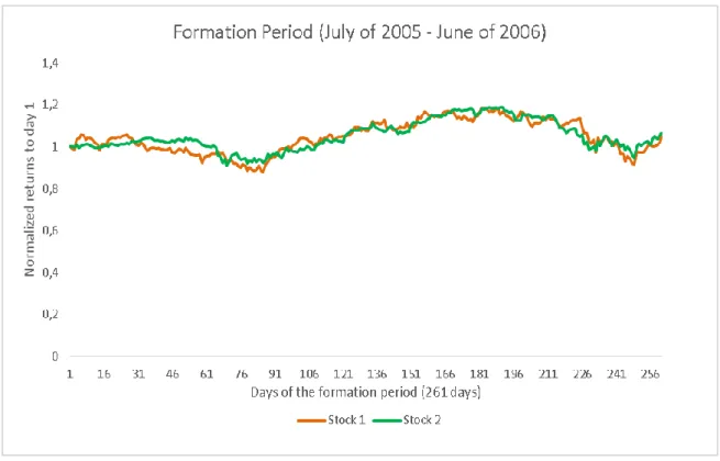
2Subsequently, by summing all these differences and sorting them from the lowest to the highest, we will have an ordered list by the closeness of stocks in the pairs. The first pair of the list is the pair that has the lower closeness measure, meaning, the pair that has the two firms with the greater relationship between each other on our formation period, and ending on the pair that has the highest closeness measure, this is, the pair that has the two firms with the worst relationship between each other on our formation period. Below, in Figure 4, we have a sample of the normalized returns to day 1 in a formation period of a pair that we used to trade:
In the figure above, we have the example of the formation period comprehended between July of 2005 and June of 2006. As we can see by the similar variations, this stock had a closeness measure really low, because the variations were stable over the period and they stayed really close from each other.
3.4 Trigger moment and decision on what position to
take
We already explained before that we open a position every time the normalized prices of the two stocks of the pair diverge more than two historical standard deviations. As we can see in Formula 4 presented below, a position is open when: (4)
|
𝑃𝑎i+1 𝑃𝑎i−
𝑃𝑏i+1 𝑃𝑏i| > ±
2
×
StDev
(
𝑃𝑎i+1 𝑃𝑎i−
𝑃𝑏i+1 𝑃𝑏i)
We know that we will short the stock that had an increase in his relative price and that we will long the stock that had a decrease in his relative price. We used the tri-state indicator variable, as exposed previously in Figure 1, in order to know what position we should take.
In Formula 5, we have the mathematically explanation:
(5)
If
𝑃𝑎𝑃𝑎i+1i
>
𝑃𝑏i+1
𝑃𝑏i
,
long on stock b and short on stock a (+1 on tri-statevariable)
If
𝑃𝑎𝑃𝑎i+1i
<
𝑃𝑏i+1
𝑃𝑏i
,
long on stock a and short on stock b (-1 on tri-statevariable)
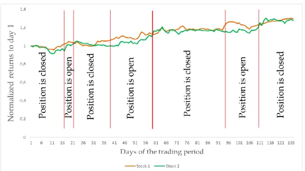
Below, in Figure 6, we have an example of the same pair we presented before in Figure 4, but now, related to its trading period:
Still, as we can see in Figure 5, we applied our strategy and we trade three times during the whole trading period. We opened a position on the day 17 and we closed on the day 22 and, as we can see in the figure, that was the day the prices crossed. Again, we opened a position on the day 40 and closed on the day 60. The third trade started on the day 94 and finished on the day 111. This serves as an example for what we did in all the trading periods of our sample.
3.5 Excess return of a position
Later, we had to compute the return of each position that opened. In order to do that, we used this simple formula:
(6)
(
𝑂𝑝𝑒𝑛 𝑝𝑟𝑖𝑐𝑒 𝑠 −𝐶𝑙𝑜𝑠𝑒 𝑃𝑟𝑖𝑐𝑒 𝑠𝑂𝑝𝑒𝑛 𝑃𝑟𝑖𝑐𝑒 𝑠+
𝐶𝑙𝑜𝑠𝑒 𝑝𝑟𝑖𝑐𝑒 𝑙 −𝑂𝑝𝑒𝑛 𝑃𝑟𝑖𝑐𝑒 𝑙𝑂𝑝𝑒𝑛 𝑃𝑟𝑖𝑐𝑒 𝑙
)
However, we can have two limitations while computing the returns for our position. The first one that may arise is when a pair, after opening, does not close until the last day of the trading period. Every time this happens, we will follow Gatev et al. (2006) and assume that we close the position on the last day of the trading period, with the price that corresponds to that same day. The second limitation that can appear is when a company is delisted from the stock exchange. In this case, we will again follow their study and use the delisting return or the last available price.
3.6 Limitations of the strategy (in general)
The strategy can face some limitations which can be avoided (or, at least, reduced) by hedge funds and financial institutions, but not so easily for a “normal” investor. We will now identify two types of limitations: technical and financial.
The technical limitation is related to entering and exiting the market. A “normal” investor doesn’t have the same conditions to access the market as a financial institution, namely the order has to be processed before being sent to the market. And, for this reason, some of the prices used to calculate the returns
may not be available when starting or ending the trading, mostly due to delays in orders being processed.
As to the financial limitations, we can see the strategy limited by problems with margin calls3. As stressed above, the strategy is based on the convergence
of prices. However, that could not happen in the first few days, or even months. If in that period, the prices continue to diverge, a margin call will be sent out by the financial institution and, if that call is not fulfilled because of liquidity problems, the position may be closed, therefore not allowing to wait for the convergence of the prices of the stocks and, thus, having to assume a negative return. In addition, a position might have to be open on several pairs at the same time, which means that funds must be available at all time.
Since the pairs trading strategy uses, at least, one long position and one short position, two other financial problems can be found. One, is that the price of taking a long and a short position is not being taken into account on the results, this is, the trading costs and fees, which will surely make the results seem better than they actually are. In addition, the differences between “normal” investors and financial institutions have again an important role, because this strategy could be profitable for investors with low trading costs and fees, but it can be shown unprofitable to “normal” investors.
3.7 Refinements
3.7.1
Specific liquidity
One aspect that was not addressed in all the studies presented was the question of the liquidity of the stocks. One stock of the pair can be really different from the other in terms of trading size and liquidity. Therefore, a liquidity problem can be found if we intent to trade the highest-valued company with the lowest-valued company since we would not be able to enter or exit the market in the exact moment we want.
To solve this question, after computed and sorted (from the lowest to the highest) the closeness variable, we restring the top 20 pairs of each formation period and we added a new restriction. To apply that restriction, first we computed the specific liquidity formula:
(7)
𝑆𝑝𝑒𝑐𝑖𝑓𝑖𝑐 𝑙𝑖𝑞𝑢𝑖𝑑𝑖𝑡𝑦
𝑡=
𝑋̅ (𝑇𝑢𝑟𝑛𝑜𝑣𝑒𝑟 𝑏𝑦 𝑣𝑜𝑙𝑢𝑚𝑒
𝑖, 𝑡∗ 𝑃𝑟𝑖𝑐𝑒
𝑖, 𝑡)
After implementing this formula, the restriction that we applied was that in the two stocks that constituted a pair, one could not be twice or half the other in their formation period in terms of specific liquidity. If, for instance, one investor wants to take a lot of positions (or invest a high quantity of money) in the above-mentioned trade, that would prove to be almost impossible to do since the liquidity of the lowest-valued company would not allow this to happen. Therefore, by implementing this specific liquidity restriction, we are dropping these, for this purpose called, “anomalous” pairs and, subsequently, it will not let us trade pairs like those.
Previously, when we dropped stocks that didn’t had more than 120 trading days in each 6 month window, we took control about liquidity problems in
general. That is to say that we had already dropped stocks that, because of their specific characteristics, didn’t attract investors to invest in them or that, due to market regulators, transactions were not allowed for a certain period of time.
Thus, now the problem was not the trading days that a company had, but it was the trading size of both firms in the pair that mattered. The specific liquidity restriction allowed us to only have pairs that, not only looked similar in terms of historical returns, but that were also really similar in their size characteristics. There could be a number of reasons to apply this restriction but the main one is that we can be forced to close a position because the stocks crossed and that may not be possible in that exact moment because the liquidity of one of the stocks might not be enough to support this process.
This is a new refinement and, from now on, we will assume that this is a restriction that cannot be ruled out from our strategy, otherwise we will have results that can’t actually be achieved.
After we applied this restriction to the top 20 pairs, we ended up with an average of 6.74 pairs per trading period. Below, in figure 5, we can see the number of pairs in each trading period:
3.7.2
Introducing bid and ask prices
As stated in section 2, all the studies presented used close prices to compute the trade, this is, they used the same price to buy and sell the stocks. However, we know that this is not the way that stocks are bought and sold in the market. To perform this action, bid and ask prices are the prices that are used to sell and buy one stock, respectively, and for this reason we added them to compute the returns of the positions.
With the introduction of bid and ask prices in our own study, we didn’t need to wait one day to open or close our position. For this purpose, we will assume that we open and close our position on the exact day that the normalized prices crossed. However, even though we solved the problem of not applying bid and ask prices in the studies presented, this brought us another problem to solve.
We used the close bid and ask prices to compute the profit/loss of our trade. This is an issue because if we only have close prices, we cannot trade in that exact day since the market is closed. This could only be solved if we had intra-day prices, which would allow us to open/close our position in the exact moment when the cross occurs. Nevertheless, intra-day prices were not accessible to us, at least, for all the period of our sample. However, even if they were, it would be a long and arduous process to compute all the returns and trades for those intra-day prices. Once having the close prices and knowing that we can’t trade after the market closes, we will assume in our study that we will open and close our position in the exact moment the market opens in the next morning but with the close price of the day before. This is not the only way to solve this problem, but it seemed the best approach.
3.7.3
Stop loss strategies
In addition to the improvements that we already made to the unconditional strategy of Gatev et al. (2006) until this point, we sought to implement some other refinements that we thought that could help us improve the efficiency of the strategy, or, at least, that would prove the robustness of our strategy. For that reason, we developed a new strategy, but now implementing stop losses for every position we took on the market. We divided these stop losses in three types: a) stop losses per days, b) stop losses per percentage of loss and c) a mix between the two mentioned before. Within each of these parameters, namely in a) we created two types of stop losses per days: i) a stop loss after 5 consecutive days in continuous loss and ii) a stop loss after 10 consecutive days in continuous loss. In b) we implemented a stop loss after the percentage of loss reached 15%. In c) we created a mix of a) and b), triggering the stop loss when we were losing for 5 consecutive days or when we reached 15% in losses.
4. Results
4.1 Unconditional strategy compared to specific
liquidity strategy
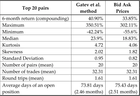
We cannot compare previous results to ours, mostly because previous studies focused on US markets and covered a different period. To calibrate our results, as much as possible, we have first implemented the strategy as close as possible to prior literature. Namely, we start by selecting the top 20 pairs without any restriction as in Gatev et al. (2006). We then implemented some modifications. The first modification was to apply a liquidity restriction (section 3.7.1) when selecting pairs. Another modification was the use of bid and ask prices, instead of the closing price (section 3.7.2). Results are in table 2 and 3:
Top 20 pairs Gatev et al. method
Bid Ask Prices
Limited pairs by specific liquidity restriction Gatev et al. method Bid Ask Prices
6-month return (compounding) 40.90% 33.85% 6-month return (compounding) 16.39% 15.39%
Maximum 350.51% 302.11% Maximum 175.63% 221.41%
Minimum -42.24% -55.6% Minimum -27.62% -30.23%
Median 23.9% 18.83% Median 18.04% 17.46%
Kurtosis 4.72 4.06 Kurtosis 7.44 9.58
Skewness 2.02 1.82 Skewness 2.29 2.74
Standard Deviation 0.95 0.82 Standard Deviation 0.44 0.55
Number of pairs (mean) 20 20 Number of pairs (mean) 6.74 6.74
Number of trades (mean) 32.31 32.31 Number of trades (mean) 10.94 10.94
Round trips (mean) 1.61 1.61 Round trips (mean) 1.60 1.60
Average days of an open position
73.81 days (2.46 months)
75.43 days (2.51 months)
Average days of an open position 75.52 days (2.52 months) 77.12 days (2.57 months)
Table 3: Results of both strategies using the limited pairs by specific liquidity restriction
Table 2: Results of both strategies using the top 20 pairs without any
First and foremost, before analysing the results, we should focus on the number of pairs we ended up by applying the specific liquidity restriction. As we already explained, that restriction was applied to the top 20 pairs (Table 2) and, in average, we ended with 6.74 pairs per trading period (Table 3). As we pointed out before, this restriction is something that we consider that has to be a part of our strategy in order to level the firms between themselves.
Looking at the results, our first conclusion is that Gatev et al. (2006) study was biased upwards, even with the addition of the “one day waiting rule”. Considering the top 20 pairs, the difference of trading using close daily price or using close bid and ask prices, was of 7.05% on the 6-month excess return (compounding). Also, as was expected, the average days that a position remains open is higher when using the bid and ask prices (2.51 months) than when using just the daily prices (2.46 months) because if a position is closed because the trading period ended, the strategy presented by Gatev et al. (2006) has less trading days, since it started one day after our strategy but closed at the same time.
We can also compare the value that was reached using daily prices (2.46 months) to the one that was found by Gatev et al. (2006) in their research for the top 20 pairs (3.76 months). Despite the differences in the time period between the two researches, we can state that trades using stocks from London Stock Exchange had fewer days with an open position than the trades with US stocks.
Nonetheless, we can go further, and compare the average number of trades per trading period between our and Gatev et al. (2006) research. In our study, we established that, on average, we had 32.32 number of trades per trading period, while they found that the average number of trades per trading period was 37.834. Again, despite the differences in the time period between the two
4 Gatev et al. (2006) doesn’t present this value on their study, however, we can try to determine an approximate
round-studies, we can assert that the average number of trades per trading period is higher in the US stocks than in the London Stock Exchange.
With regard to the elements referred, it may be pointed out that by changing from “top 20 pairs” to specific liquidity pairs, the number of round trips stayed almost the same (1.62 and 1.60, respectively). The number of trades reduced as a consequence of having less pairs (32.32 to 10.95, respectively) and the average number of days with an open position increased in, approximately, 2 days, which means that the pairs that were deleted had an average number of days with an open position lower than the pairs that we ended up after the specific liquidity restriction. Also, the standard deviation of the results is reduced in this process, which means that the risk of our strategy also reduced.
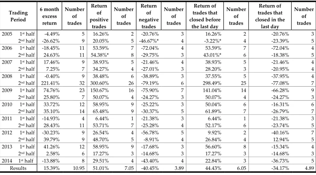
4.2 Profit/Losses: Where are they coming from?
Considering that strategies that use daily prices are biased upwards and that strategies that don’t include a specific liquidity restriction are not possible to carry out (or, at least, we will always assume the risk of not being corresponded on the market), the most appropriate is the strategy that includes the specific liquidity restriction and, at the same time, uses the bid and ask prices. Following the presented results of the strategy with limited pairs, we wanted to understand where our profits/losses came from.
Thus, we divided our results in 2 groups, which were:
Return of positive trades and return of negative trades;
Return of trades that closed before the last day and return of trades that closed in the last day.
Trading Period 6 month excess return Number of trades Return of positive trades Number of trades Return of negative trades Number of trades Return of trades that closed before
the last day
Number of trades Return of trades that closed in the last day Number of trades 2005 1st half -4.49% 5 16.26% 2 -20.76% 3 16.26% 2 -20.76% 3 2nd half -26.62% 9 20.05% 5 -46.67%* 4 -3.22%* 4 -23.39% 5 2006 1st half -18.45% 11 53.59% 7 -72.04% 4 53.59% 7 -72.04% 4 2nd half 24.63% 11 54.38%* 8 -29.75% 3 43.01%* 6 -18.38% 5 2007 1st half 17.46% 9 38.93% 5 -21.46% 4 38.93% 5 -21.46% 4 2nd half 7.25% 7 34.27% 4 -27.01% 3 28.20% 3 -20.95% 4 2008 1st half -0.40% 9 38.48% 6 -38.89% 3 37.55% 5 -37.95% 4 2nd half 221.41% 32 300.60% 26 -79.19% 6 298.49% 25 -77.08% 7 2009 1st half 74.76% 23 150.67% 16 -75.90% 7 141.04% 14 -66.28% 9 2nd half 25.80% 7 50.07% 4 -24.27% 3 50.07% 4 -24.27% 3 2010 1st half 33.72% 12 58.95% 9 -25.22% 3 50.04% 6 -16.31% 6 2nd half 35.10% 14 65.48% 9 -30.37% 5 61.89% 7 -26.79% 7 2011 1st half -14.93% 4 6.44% 1 -21.38% 3 6.44% 1 -21.38% 3 2nd half 28.43% 11 53.71% 7 -25.28% 4 52.17% 6 -23.74% 5 2012 1st half -30.23% 9 26.54% 4 -56.78% 5 9.92% 2 -40.16% 7 2nd half 39.79% 9 48.70% 5 -8.91% 4 26.84% 4 12.94% 5 2013 1st half 41.26% 12 58.95% 9 -17.68% 3 56.60% 8 -15.34% 4 2nd half 2.58% 6 17.27% 3 -14.68% 3 17.27% 3 -14.68% 3 2014 1st half -13.88% 8 29.51% 4 -43.40% 4 22.84% 3 -36.73% 5 Results 15.39% 10.95 51.01% 7.05 -40.45% 3.89 44.43% 6.05 -34.17% 4.89
After examining table 4, we can conclude that the number of trades that ended with profit (7.21) was higher than the number of trades that ended with a loss (3.74). However, this does not need to happen for the success of the strategy. We could lose in most positions if that loss is compensated by the positions we won.
Moreover, the number of trades that closed before the last day of the trading period (6.05) was higher than the number of trades that closed in the last day of the trading period (4.89). However, even more relevant, is to look at the returns of this two items. The trades that closed in the last day of the trading had a 6-month excess return (compounding) of -34.17%. We can point out two reasons for this bad outcome: one of them is that some pairs open near the end of the trading period and don’t have time to converge, thus having a bad result. The other reason is that some pairs open in the beginning of the trading period and keep diverging from the point we opened and never converge until the end of the trading period.
We should also take into account the results of trades that closed before the last day of the trading period. Of course, this result would be positive (44.43%) because if the position was closed before the last day of the trading period, it is because the normalized prices of the two stocks converged and crossed, meaning that we had profit in all the situations where we closed before the last day (except the pairs that were forced to close because one of the firms was delisted from the index).
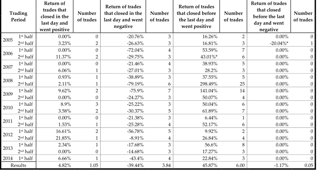
Additionally, inside of this last group, we divided it again in two new groups, which were:
• Return of trades that didn't close before the last day and went positive and return of trades that didn't close before the last day and went negative;
• Return of trades that closed before the last day and went positive and return of trades that closed before the last day and went negative.
Trading Period
Return of trades that closed in the
last day and went positive
Number of trades
Return of trades that closed in the last day and went
negative
Number of trades
Return of trades that closed before
the last day and went positive
Number of trades
Return of trades that closed before the last
day and went negative Number of trades 2005 1 st half 0.00% 0 -20.76% 3 16.26% 2 0.00% 0 2nd half 3.23% 2 -26.63% 3 16.81% 3 -20.04%* 1 2006 1 st half 0.00% 0 -72.04% 4 53.59% 7 0.00% 0 2nd half 11.37% 2 -29.75% 3 43.01%* 6 0.00% 0 2007 1 st half 0.00% 0 -21.46% 4 38.93% 5 0.00% 0 2nd half 6.06% 1 -27.01% 3 28.2% 3 0.00% 0 2008 1 st half 0.93% 1 -38.89% 3 37.55% 5 0.00% 0 2nd half 2.11% 1 -79.19% 6 298.49% 25 0.00% 0 2009 1 st half 9.62% 2 -75.9% 7 141.04% 14 0.00% 0 2nd half 0.00% 0 -24.27% 3 50.07% 4 0.00% 0 2010 1 st half 8.9% 3 -25.22% 3 50.04% 6 0.00% 0 2nd half 3.58% 2 -30.37% 5 61.89% 7 0.00% 0 2011 1 st half 0.00% 0 -21.38% 3 6.44% 1 0.00% 0 2nd half 1.53% 1 -25.28% 4 52.17% 6 0.00% 0 2012 1 st half 16.61% 2 -56.78% 5 9.92% 2 0.00% 0 2nd half 21.85% 1 -8.91% 4 26.84% 4 0.00% 0 2013 1 st half 2.34% 1 -17.68% 3 56.6% 8 0.00% 0 2nd half 0.00% 0 -14.68% 3 17.27% 3 0.00% 0 2014 1st half 6.66% 1 -43.4% 4 22.84% 3 0.00% 0 Results 4.82% 1.05 -39.44% 3.84 45.87% 6.00 -1.17% 0.05
Many conclusions can be drawn regarding this table. The first one is that, per each trading period, in average, 1.05 trades closed in the last day of the period and were profitable (with an average 6-month excess return of 4.82%). Also, per trading period, in average, 6 trades closed before the last day of the trading period and were profitable (with an average 6-month excess return of 45.87%).
Besides that, we should also observe the trades that ended with a negative return. On average, per trading period, 3.84 trades closed in the last day of the period and had a negative return (average 6-month excess return of -39.44%). Also, on average, per trading period, 0.05 trades closed before the last day and had a negative return (average 6-month excess return of -1.17%). During all our trading periods, this only happened one time and it was due to the fact that we were forced to close a pair because one of the firms that constituted that pair was delisted from the index.
However, this situation of having a stock of a pair delisted from the index, while they were part of our tradable pairs, happened two times: the one mentioned above, and the other in the second half of 2006, as can be seen on table 5 (anyway, that trade ended up with a positive return).
4.3 Specific
liquidity
restriction
strategy
and
introduction of stop losses
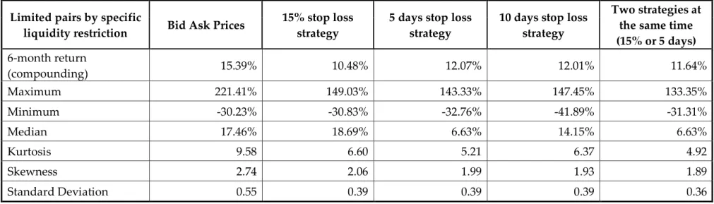
After a detailed analysis of our profits and losses, we intended to see if we could improve our results and, for that reason, we applied the stop losses presented before (section 3.7.3) to this strategy and the results can be seen below, in Table 6:
Limited pairs by specific
liquidity restriction Bid Ask Prices
15% stop loss strategy
5 days stop loss strategy
10 days stop loss strategy
Two strategies at the same time (15% or 5 days) 6-month return (compounding) 15.39% 10.48% 12.07% 12.01% 11.64% Maximum 221.41% 149.03% 143.33% 147.45% 133.35% Minimum -30.23% -30.83% -32.76% -41.89% -31.31% Median 17.46% 18.69% 6.63% 14.15% 6.63% Kurtosis 9.58 6.60 5.21 6.37 4.92 Skewness 2.74 2.06 1.99 1.93 1.89 Standard Deviation 0.55 0.39 0.39 0.39 0.36
Table 6:Results of the limited pairs’ strategy with the bid and ask prices and results of the same strategy with the inclusion of 4 different stop loss strategies
After analysing these results we can assert that none of the strategies with stop losses increased the returns and, therefore, two conclusions emerge. The first one is that none of the strategies proved to be useful to maximize our returns (as can be seen in the returns of each strategy in table 6). However, the market works on a risk/return binomial, where to get a higher return, we need to face a higher risk. Thus, this strategies can be valid if the goal of the investor is to reduce the risk, something that was achieved with the reduction of the standard deviation. The second one is that these results proved the robustness of our strategy. As we introduced in the beginning of our study, after the normalized prices of two stocks of a pair diverged by more than two historical standard deviations, we opened a position and we waited until the moment the existed difference disappeared due to the convergence of the normalized prices. Thus, if the stop losses reduced the returns of the strategy, we can assume that, in most trades, the prices converged after a position was open.
As we can see above in Table 6, all the strategies limited our returns, being the “5 days stop loss strategy” the less harmful. Nevertheless, this strategy is still reducing our returns in 3.32%. The “15% stop loss strategy” is the one that presents the worst results of all. Therefore, the “10 days stop loss strategy” had returns that were near the “5 days stop loss strategy”, but still performed worse than this one.
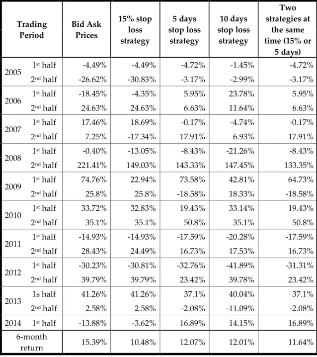
4.4 Detailed results of the strategies
It is now the time for a deeper analysis and to examine the results by trading periods. Below, on table 7, we have the results divided by trading periods and by strategies. Trading Period Bid Ask Prices 15% stop loss strategy 5 days stop loss strategy 10 days stop loss strategy Two strategies at the same time (15% or 5 days) 2005 1 st half -4.49% -4.49% -4.72% -1.45% -4.72% 2nd half -26.62% -30.83% -3.17% -2.99% -3.17% 2006 1 st half -18.45% -4.35% 5.95% 23.78% 5.95% 2nd half 24.63% 24.63% 6.63% 11.64% 6.63% 2007 1 st half 17.46% 18.69% -0.17% -4.74% -0.17% 2nd half 7.25% -17.34% 17.91% 6.93% 17.91% 2008 1 st half -0.40% -13.05% -8.43% -21.26% -8.43% 2nd half 221.41% 149.03% 143.33% 147.45% 133.35% 2009 1 st half 74.76% 22.94% 73.58% 42.81% 64.73% 2nd half 25.8% 25.8% -18.58% 18.33% -18.58% 2010 1 st half 33.72% 32.83% 19.43% 33.14% 19.43% 2nd half 35.1% 35.1% 50.8% 35.1% 50.8% 2011 1 st half -14.93% -14.93% -17.59% -20.28% -17.59% 2nd half 28.43% 24.49% 16.73% 17.53% 16.73% 2012 1 st half -30.23% -30.81% -32.76% -41.89% -31.31% 2nd half 39.79% 39.79% 23.42% 39.78% 23.42% 2013 1s half 41.26% 41.26% 37.1% 40.04% 37.1% 2nd half 2.58% 2.58% -2.08% -11.09% -2.08% 2014 1st half -13.88% -3.62% 16.89% 14.15% 16.89% 6-month return 15.39% 10.48% 12.07% 12.01% 11.64%