UNIVERSIDADE DE ÉVORA
DEPARTAMENTO DE ECONOMIA
DOCUMENTO DE TRABALHO Nº 2008/05
OctoberIs Fuel-Switching a No-Regrets Environmental Policy?
VAR Evidence on Carbon Dioxide Emissions, Energy Consumption and
Economic Performance in Portugal
Alfredo Marvão Pereira * Department of Economics,
College of William and Mary, Williamsburg, VA 23187
Rui Manuel Marvão Pereira ** Thomas Jefferson Program in Public Policy College of William and Mary, Williamsburg, VA 23187
UNIVERSIDADE DE ÉVORA
DEPARTAMENTO DE ECONOMIA
Largo dos Colegiais, 2 – 7000-803 Évora – Portugal Tel. +351 266 740 894 Fax: +351 266 740 807
www.decon.uevora.pt [email protected]
* Email: [email protected] ** Email: [email protected]
Resumo/Abstract:
The objective of this paper is to estimate the impact of carbon dioxide emissions from fossil fuel combustion activities on economic activity in Portugal in order to evaluate the economic costs of policies designed to reduce carbon dioxide emissions. We find that energy consumption has a significant impact on macroeconomic activity. In fact, a one ton of oil equivalent permanent reduction in aggregate energy consumption reduces output by €6,340 over the long term, an aggregate impact which hides a wide diversity of effects for different fuel types. More importantly, and since carbon dioxide emissions are linearly related to the amounts of fuel consumed, our results allow us to estimate the costs of reductions in carbon dioxide emissions from different energy sources. We estimate that marginal abatement costs for carbon dioxide are €45.62 per ton of carbon dioxide per year for coal, €66.52 for oil, €91.07 for gas, €191.13 for electricity and €254.23 for biomass. An important policy implication is that, once the overall economic costs of reducing carbon dioxide emissions are considered, fuel switching is a no-regrets environmental policy capable of reducing carbon dioxide emissions without jeopardizing economic activity and indeed with the potential for generating favorable economic outcomes
Palavras-chave/Keywords: carbon dioxide emissions, energy and the economy, environmental policy, fuel-switching, vector autoregressive model
1
1. Introduction
Carbon dioxide emissions from fossil fuel combustion in Portugal reached 56.950 Mt
CO2 in 2006, according to the Agencia Portuguesa do Ambiente (2006a) (Portuguese
Institute for the Environment, APA hereafter). For the period 1990-2006 they account for
96.2% of total greenhouse gas emissions in the energy sector – the remainder being
methane and nitrogen oxide emissions, and for 68.5% of total greenhouse gas emissions -
the remainder being due to industrial processes, fugitive emissions from fuels, solvent
and other product use, agriculture, and waste.
Environmental policies to reduce carbon dioxide emissions from fossil fuel
combustion have traditionally focused on investment in research, development, and
deployment of energy-efficient technologies, on restructuring the composition of fuel
demand, and on reducing energy consumption. Naturally, the choice and design of such
policies is bound to have an important impact on economic activity [see, for example,
Manne and Richels (1992), Nordhaus (1993), Grubb et al. (1993), Gaskins and Weyant
(1993), Zhang and Folmer (1998), Jorgenson (1998), Hue and Xu (2000) and Lasky
(2003)]. Furthermore, not all policy alternatives are equally feasible in general and much
more so in the case of a small economy like Portugal.
Energy-efficiency improvements have the potential for bringing significant gains in
productivity while reducing the consumption of fossil fuels and greenhouse gas emissions
2 is rather limited. The development of energy-efficient technologies is more of a
long-term prospect and more outside the scope of small or developing economies. Ultimately,
policy instruments that promote fuel switching tend to be the policies of choice.
International studies, however, have often concluded that the fuel switching necessary to
ensure deep cuts in emissions would increase direct energy system costs as a result of a
regulatory-induced shift to more expensive but cleaner fuels. This highlights the
perceived trade-off between reducing carbon dioxide emissions from fossil fuel
combustion activities and economic growth [see, for example, Chen et al. (2005)].
The objective of this paper is to contribute to the design of environmental policy
instruments, and particularly, fuel-switching policies, which minimize the economic costs
of regulation while effectively reducing emissions. We do so by focusing on the
economic impact of final energy demand by type. Then, since carbon dioxide emissions
are linearly related to the amounts of fuel consumed, our estimates of the economic
impact of energy consumption allow us to estimate the marginal abatement costs for
carbon dioxide emissions from fossil fuel combustion by energy source and gain an
appreciation of the costs of policies directed at specific emission sources.
We obtain the economic impact of energy demand by estimating a series of vector
auto-regressive (VAR) models relating output, employment and private investment to
aggregate energy demand or disaggregate energy demand for different types of energy.
This allows us to highlight the dynamic feedback mechanisms among the different
variables and captures both direct and indirect channels through which energy
consumption affects output. As an input to production, energy directly affects output. On
3 - capital and labor. To this effect, empirical evidence suggests that during periods of high
energy prices, the tendency is for firms to switch to less energy-intensive capital
equipment and for more labor-intensive industries to develop [see, for example,
Jorgenson (1998)].
Our methodological approach follows very much the recent trends in the literature.
Recent advances in times-series analysis have stimulated research into the nature of the
relationship between energy consumption and economic activity via the concept of
Granger-causality [see, for example, Masih and Masih (1996), Cheng and Lai (1997),
Asafu-Adjaye (2000), Stern (1993, 2000), and Oh and Lee (2004)]. Although the general
results are mixed, the importance of the dynamic relationship between energy
consumption and output is clear. In fact, bi-directional causality has served as the basis
for generating forecasts of energy consumption based, at least partially, on the level of
economic activity [see, for example, Crompton and Wu (2005), Francis et al. (2007), and
Perobelli et al (2007)]. As a result, vector auto-regressive models have become a standard
approach for forecasting energy consumption [see, for example, Energy Information
Administration (2002)].
Our paper extends the literature to consider the impact of shocks to the demand for
specific types of energy due to climate policy measures on output, employment and
private investment. Climate policy induced reductions in energy consumption generate a
series of responses in economic activity which define the economic costs of regulation.
As a result, we can consider not only the carbon content of the fuel when designing
policies to reduce greenhouse gas emissions, but the impact of that source of energy on
4 compliance with environmental regulation and better understand the economic costs of
fuel switching policy measures.
2. Data and Preliminary Empirical Results
This section describes the basic data set, presents the results of the unit root and
cointegration tests, and addresses the issue of VAR model specification.
2.1Data: sources and description
We use annual data for the period 1977 to 2003 for output, employment, and private
investment, as well as aggregate and disaggregated final demand for energy. Because
this sample period includes years before and after Portugal joined the European Union in
1986, we consider throughout the empirical analysis the possibility of a structural break
in 1986. Economic data was obtained from the Banco de Portugal (1997), Commission of
the European Communities (1999) and Ministério das Finanças (2006). Data for final
demand for energy was obtained from the Energy Balance Sheets published by Direcção
Geral de Energia (Portuguese Department of Energy, DGE hereafter) and is measured in
103 tons of oil equivalent (toe hereafter). Aggregate final demand for energy is defined as
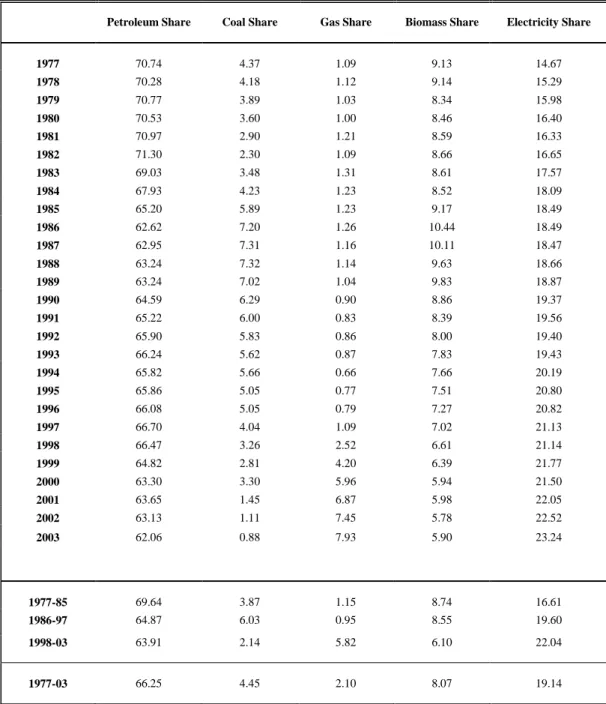
the sum of final demand for petroleum and its derivatives, coal, gas, biomass, and
electricity. See Table 1 for the evolution of the composition of the final demand for
energy.
Data for the final demand for energy products is compiled and published by the DGE.
5 distinction between primary and final energy demand. As a result, the DGE makes
available two data sets – one for the period between 1971 and 1993 and another for the
period between 1990 and 2003 - with a four-year overlap. The data collection
methodology and presentation differs significantly between the two periods and in order
to ensure consistency between the two series, several methodological issues are taken
into consideration as will be mentioned below.
The data for petroleum and its derivatives includes liquefied petroleum gas, gasoline,
diesel and fuel oil. Although the dominant use of petroleum and its derivates is as an
energy source, they are also used as raw materials in the production of, for example,
plastics and asphalt. Petroleum derivatives used as raw materials are not considered in
our data, with the exception of fuel oil. This is because prior to 1985 the DGE accounting
methodology did not distinguish between fuel oil used for energy and non-energy
purposes. Petroleum and its derivatives account for an average of 66.3% of total final
energy demand for the sample period and show a declining trend from 69.6% between
1977 and 1985 to 63.9% in the final years of the sample period.
The data on final demand for coal includes domestic production and imports of
anthracite and bituminous coal. This data set is rather consistent methodologically
throughout the sample period and therefore no adjustments to the published data were
necessary. Coal constitutes 4.5% of total final energy demand for the sample period. Its
weight in total final energy consumption has shown some fluctuations, starting at 3.9% in
the beginning of the sample period reaching a high of 6.0% for 1986 to 1997 and
decreasing to 2.1% in the last five years of the sample period. The virtual extinction of
6 low grade anthracite closed in 1994 - largely contributed to the steady decline in coal
consumption, particularly after 1986.
Data for gas includes coke gas, blast furnace gas, city gas and natural gas. Natural gas
distribution infrastructure developed rapidly after 1998 to become an important
component of the energy system in Portugal. The demand for gas itself has increased
significantly with the introduction of natural gas. In fact, the average share of gas in total
final energy consumption for the period 1977-1985 was 1.2% and rose to 5.8% between
1998 and 2003. Gas consumption grew, on average, at an average annual rate of 24.1%
after the introduction of natural gas in 1998. In our empirical analysis below we fully
consider the possibility of a structural break in 1998 consistent with the introduction of
natural gas.
Final demand for biomass includes registered purchases up until 1993, after which,
data is based upon household surveys and thus reports both purchases and collection of
biomass and forest waste. In order to generate a consistent series in levels, the growth
rate of biomass consumption after 1990 is applied to the earlier level data. We find that
the implied growth rate during the overlapping period 1990-1993 is consistent, albeit
with relatively insignificant deviations. The use of biomass has decreased in relative
importance over the sample period. Between 1977 and 1985, biomass consumption
represents 8.7% of total final energy demand while in the final years of the sample period
biomass consumption accounts for only 6.1% of total final energy demand.
Data for electricity consumption includes cogeneration and heat until 1993, after
which they are accounted for separately. The level values for the overlapping years of
7 show larger variability in the order of 20%. As such we consider level data for electricity
generation until 1993 after which the new data in growth rates is considered to extend
this series. Electricity demand has grown in terms of its relative importance in total
energy consumption. It represents 16.6% of total final energy demand between 1977 and
1985 and 22.0% for the last years of the sample period.
2.2Unit root and cointegration analysis
This section considers the main results from the unit root and cointegration tests. We
use the Augmented Dickey-Fuller (ADF) t-test to test the null hypothesis of a unit root in
the different variables. The optimal lag structure is chosen using the BIC, and
deterministic components and 1986 and 1998 dummies were included if statistically
significant.
We started by applying the ADF t-tests to output, employment, private investment
and aggregate as well as each of the different types of energy consumption, in log-levels,
and consistently found that we cannot reject the null hypothesis of non-stationarity at the
5% level of significance – see Table 2. We then tested for stationarity of all the variables
in growth rates – see also Table 2. The ADF t-tests suggest that the null hypothesis of a
unit root in the growth rates can be rejected for all variables at the 5% significance level.
We take this evidence as a strong indication that stationarity in growth rates is a good
approximation for all variables.
We also test for cointegration among the different variables - output, employment,
private investment and each one of the energy variables. Due to our relatively small
8 procedure to the small sample bias toward finding cointegration when it does not exist
[see, for example, Gonzalo and Lee (1998) and Gonzalo and Pitarakis (1999)].
Following the standard Engle-Granger procedure, we perform four tests for each of
the six cases - aggregate analysis and disaggregated for each of the five types of energy -
each one with a different endogenous variable. This is because it is possible that one of
the variables enters the cointegrating relationship with a statistically insignificant
coefficient. In this case, a test that uses such a variable as the endogenous variable would
not detect cointegration. The optimal lag structure was chosen using the BIC, and
deterministic components and 1986 and 1998 dummies were included if statistically
significant. We apply the ADF t-test to the residuals of the different regressions. Test
results – see Table 3 - uniformly suggest that at the 5% level of significance it is not
possible to reject the null hypothesis of no-cointegration.
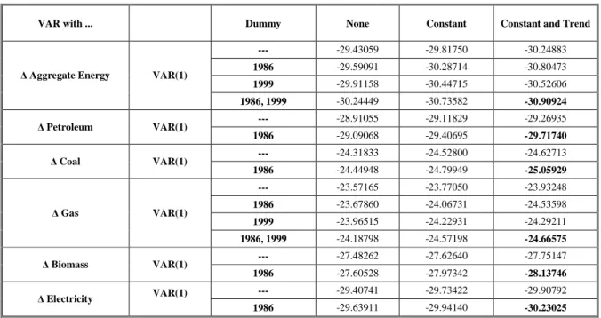
2.3VAR specifications and estimates
We have determined that all of the variables in log-levels are stationary in growth
rates and that they are not cointegrated. Accordingly, we follow the standard procedure
in the literature and determine the specifications of the VAR models in growth rates of
the original variables.
We estimate six VAR models, all of which include output, employment and
investment. In addition, each of the models includes an energy variable – aggregate
energy demand or one of five different types of energy demand. The model specifications
are determined using the BIC - see the test results on Table 4. In terms of the
9 specification with a constant and a trend. Also, we find that the best VAR specifications
include in all cases a structural break in 1986 and, in the cases of the aggregate model and
of the model for gas, a structural break in 1998 as well.
3. Identifying and Measuring the Effects of Energy Demand Shocks
We use the impulse-response functions associated with the estimated VAR models to
examine the effects of innovations in energy demand. This methodology allows dynamic
feedbacks among the different variables to play a critical role, both in the identification of
the shocks in energy demand and in measuring the effects of such shocks.
3.1Identifying shocks in energy demand
The key methodological issue in determining the effects of energy demand on
economic performance is identifying shocks in energy demand that are truly exogenous,
i.e., that are not contemporaneously correlated with innovations in the remaining
variables. We have in mind shocks induced by the introduction of environmental
regulation, from, for example, the policy instruments considered within the APA’s
National Program for Climate Change (2006b) for Portugal with the objective of reducing
carbon dioxide emissions from fossil fuel combustion activities. In dealing with this
issue, we draw from the standard approach in the monetary policy literature [see, for
example, Christiano, Eichenbaum and Evans (1996, 1998), and Rudebusch (1998)]
10 The econometric counterpart to this idea is to imagine a policy function, which relates
the rate of growth of energy demand to the relevant information set. In our case, the
relevant information set includes past and current observations of the growth rates of
output, employment and private investment. The residuals from this policy function
reflect the unexpected component of the growth in energy demand and are uncorrelated
with innovations in the other variables.
In the central case, we assume that the relevant information set for energy demand
includes past but not current values of the other variables. This is equivalent, in the
context of the standard Choleski decomposition, to assuming that shocks in energy
demand lead shocks in the other variables. As such, shocks in energy demand induced by
environmental regulation designed to reduce carbon dioxide emissions, while affecting
contemporaneously the economic performance of the economy are not affected
contemporaneously by such economic performance. This identification strategy seems to
be rather reasonable conceptually. Furthermore, when current values of the other
variables are included in the policy functions, in no case are such variables statistically
significant. This suggests that our identification strategy is rather reasonable also from a
statistical perspective. Nevertheless, and for the sake of completeness, when we report
our general results we also include the range of results across all alternatives within the
Choleski decomposition framework.
The policy functions for aggregate energy demand as well as the different types of
energy demand are reported in Table 5. These policy functions relate the growth in the
energy demand variables to the evolution of output, employment and private investment,
11 changes in energy demand are positively correlated with lagged changes in output and
that most of the other effects are not statistically significant – changes in private
investment seem to have significant lagged negative effects in the case of coal and
biomass and positive in the case of petroleum, but these effects seem to cancel out and do
not persist at the aggregate level.
3.2Measuring the effects of innovations in energy demand variables
We consider the macroeconomic impact of a one percentage point, one-time shock to
the rates of growth of the different types of energy demand. We expect these shocks to
have at least temporary effects on the growth rates of the other variables. However, even
temporary effects on the growth rates of the other variables translate into long-term
permanent level effects for these variables. The impulse-response functions associated
with the VAR estimates and the policy functions described above as well as the
corresponding 90% bands that characterize the likelihood shape are presented in Figures
1 – 6. We observe that without exception the accumulated impulse response functions
converge within a very short time period suggesting that most of the growth rate effects
occur within the first few years after the shocks occur.
The error bands surrounding the point estimates for the accumulated impulse
responses convey uncertainty around estimation and are computed via bootstrapping
methods. We consider 90% intervals although bands that correspond to a 68% posterior
probability are the standard in the literature (Sims and Zha, 1999). Employing one
standard deviation bands narrows the range of values that characterize the likelihood
12 nominal coverage distances may under represent the true coverage in a variety of
situations (Kilian, 1998). Nevertheless, the corresponding 90% error bands for our
accumulated impulse response functions display a high degree of precision in our
estimates. It is important to highlight that our estimates for the effect of innovations in
coal demand show a range of variation that reinforce the very small impact it has on the
economy and includes zero effects.
We estimate the long-term elasticities of the different economic variables with respect
to each type of energy demand. The long-term refers to the time horizon over which the
growth effects of the innovations disappear, i.e., the accumulated impulse-response
functions converge. The accumulated elasticities, therefore, represent the long-term
accumulated percentage point changes in the different variables for one long-term
accumulated percentage point change in energy demand once all the dynamic feedback
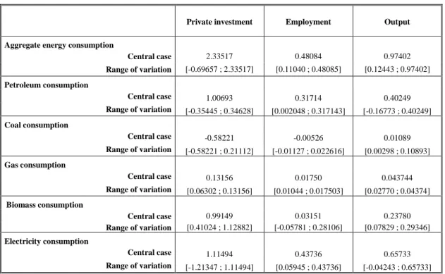
effects have been considered. The estimated elasticities are reported in Table 6.
In turn, the corresponding marginal products measure the changes - in thousands of
euros in private investment and output and in the number of long-term permanent jobs -
for a one ton of oil equivalent accumulated increase in final energy demand. We obtain
these figures by multiplying the average ratios of private investment, employment and
output to energy demand, for the last ten years, by the corresponding elasticities. The
decision to consider the average of the past ten years is designed to reflect the relative
scarcity of final demand for the various types of energy considered without letting these
ratios be overly affected by business cycle variations. Given the introduction of natural
gas in 1998 and the sharp decline in the Portuguese coal mining industry in the last
13 five years of the sample. The estimated marginal products are reported in Table 7. See
section 6 below for a discussion of the sensitivity of our results to the period chosen for
the computation of the marginal effects.
4. On the Economic Effects of Shocks in Energy Demand
Within our methodological framework, changes in final energy demand affect
economic performance throughout time while, simultaneously, changes in output,
employment and investment affect energy demand through the policy function. The
results we now present represent the final outcome of this dynamic process and fully
incorporate all of the dynamic feedbacks resulting from the initial exogenous innovation
in the relevant energy demand variable.
4.1Effects of shocks to aggregate energy consumption
The top section of Table 7 presents the effects of an exogenous shock to aggregate
final energy demand on private investment, employment and output. The empirical
results suggest that, over the long-term, energy demand crowds in both private
investment and employment. The elasticity of private investment with respect to
aggregate energy demand is 2.34, which corresponds to a long-term marginal product of
€3,550 per toe of final energy demand. In turn, the elasticity of employment with respect
to aggregate energy demand is 0.48 which suggests that, over the long term, 0.0083
permanent jobs are created for each additional toe of final energy demand (or 1 job per
14 output over the long-term with an estimated elasticity of output with respect to energy
demand of 0.97, which corresponds to a long-term marginal product of €6,340 per toe.
Our results for the impact of shocks to aggregate energy demand on employment and
output suggest that energy demand has a positive influence on long-term labor
productivity in the economy. As such, the long-term responsiveness of output is greater
than the long-term responsiveness of employment. Specifically, in the long term the
labor-output ratio in the economy responds to shocks to energy demand with an elasticity
of 0.49.
4.2Effects of shocks to different types of energy consumption
Having established that aggregate energy demand has a significant impact on
economic performance, and in order to facilitate compliance with environmental
regulation and appreciate the potential costs associated with fuel switching measures, it is
important to identify the oeconomic impact of the various sources of energy individually.
Indeed, the aggregate effects of energy demand on private investment, employment and
output hide a wide diversity of effects by type of energy. Consider again Table 7 and note
that while all of the sources of energy show a strong and statistically significant impact
on macroeconomic activity the effect of coal on economic activity may be overstated.
Private investment generally responds positively to exogenous shocks in most types
of energy demand. The strongest effects come from shocks to electricity, petroleum, and
biomass demand, with elasticities of 1.11, 1.01, and 0.99. In turn, the elasticity of private
investment with respect to shocks in gas consumption is substantially smaller at 0.13 and
15 In terms of the marginal effects on private investment, biomass and electricity
consumption have the largest impact with long-term marginal products of €22,710 and
€7,900 per toe, respectively. Gas and petroleum consumption have a smaller, yet
important impact on private investment activities, increasing private investment by
€3,056 and €2,360 per toe respectively. Coal demand, however, reduces private
investment by €4,265.
Exogenous shocks to energy demand have an important impact on employment levels
as well. The strongest effect results from electricity consumption with an elasticity of
0.44, followed by petroleum consumption, with an elasticity of 0.32, biomass
consumption with 0.03 and gas consumption with 0.02. On the other hand, the estimated
elasticity of employment with respect to coal consumption is small and negative with a
value of -0.01.
Exogenous shocks in the demand for electricity have the largest impact on
employment in terms of the marginal effects of shocks to final energy demand. An
increase in electricity consumption creates 0.0348 new jobs per toe (1 job per 28.7 toe).
In turn, shocks in the demand for petroleum and biomass generate 0.0084 and 0.0083
new jobs per toe, respectively (1 job per 119.0 and 120.5 toe) while an increase in gas
consumption by a toe corresponds to the creation of 0.0044 new jobs over the long-term
(1 job per 227.3 toe). As with private investment, increased coal consumption has a
negative impact on employment, leading to a loss of 0.0042 jobs (1 job per 238.1 toe).
Given the impact of each type of energy on private investment and employment, the
relative importance of their impact on output is no surprise. Electricity consumption has
16 respect to petroleum and biomass consumption are 0.40 and 0.24, respectively. In turn,
the output elasticities of gas consumption and coal consumption with respect to output
are much smaller at 0.04 and 0.01, respectively. The positive impact of coal on output
highlights uncertainty in the parameter estimates, particularly when we consider the
negative impact induced by the final demand for coal on private investment and
employment. This reflects the fact that the error bands surrounding the point estimates for
coal include zero.
Of the various types of energy considered, shocks to the demand for biomass and
electricity have the largest impact on output in terms of their marginal products. Increases
in final demand for biomass and electricity by a toe generate a long term increase in
output of approximately €23,340 and €19,950, respectively. The remaining effects are
substantially smaller. The effects of increased gas and petroleum consumption on output
are €4,257 and €4,040 per toe, respectively. Coal consumption increases output by
€3,332 per ton but may in fact have a substantially smaller effect.
5. On the Effects of Reductions in Carbon Dioxide Emissions
The economic impact of policies to reduce carbon dioxide emissions from fossil fuel
combustion activities will depend on the type of energy that is targeted by regulation.
Thus, the impact of each type of energy on the macroeconomic variables considered is
central to estimating the economic costs of fuel switching measures.
Reducing carbon dioxide emissions from fossil fuel combustion activities requires a
17 mentioned above, this can be achieved through a direct reduction in the quantity of fuel
consumed or through fuel-switching. This section seeks to explore the relationship
between fuel consumption, carbon dioxide emissions and economic performance by
estimating marginal abatement costs for carbon dioxide emissions resulting from
reductions in fossil fuel consumption from policies targeting specific sources of energy.
5.1On the carbon content of different fossil fuels
The hydrogen and carbon contained in fossil fuels generates the potential for heat and
energy production. Carbon is released from the fuel upon combustion; 99.0% of the
carbon released from the combustion of petroleum, 99.5% from natural gas, and 98.0%
from coal, oxidizes to form carbon dioxide. Thus, the carbon emitted from fossil fuel
combustion activities, once oxidized, can be used to compute the carbon dioxide
emissions by considering the ratio of the molecular weight of carbon dioxide to carbon.
Together, the quantity of fuel consumed, its carbon factor, oxidation rate, and the ratio of
carbon dioxide to carbon are used to compute the amount of carbon dioxide emitted from
fossil fuel combustion activities in a manner consistent with the Intergovernmental Panel
for Climate Change (2006) reference approach. These considerations suggest a linear
relationship between carbon dioxide emissions and fossil fuel combustion activities.
Table 8 presents the relevant information for determining the carbon dioxide emission
factor for each source of energy under consideration. We convert tons of oil equivalent
units to tera-joules of energy to ensure that that the carbon emission factor is in the
appropriate units. We then adjust for incomplete combustion via the oxidation rate and
18 we are ultimately interested in the quantity of carbon dioxide released into the
atmosphere, we multiply the quantity of carbon by 44/12, the ratio of the molecular
weight of carbon dioxide (CO2 – 12 + 16 (2)) to carbon (12).
This information allows us to determine the impact of reducing carbon dioxide
emissions from fossil fuel combustion activities through a reduction in each of the types
of energy considered. We determine the aggregate impact over a twenty year period and
present results on an annual basis. Petroleum combustion generates 3.04 tons of CO2 per
toe. Coal contains the largest quantity of carbon and as a result generates 4.04 t CO2 per
toe. Natural gas, on the other hand, contains the least carbon relative to its hydrogen
content and therefore has the lowest emission factor generating 2.34 t CO2 per toe.
In specific circumstances the carbon released upon the combustion of biomass may be
equal the carbon uptake of the sink during growth and as such biomass combustion as a
fuel source is not included in the national greenhouse gas inventories. As a result, a
closed circuit of biomass growth and combustion to satisfy energy demand is often
recommended as an appropriate method for reducing greenhouse gas emissions.
Although not constrained by climate policy, the effective utilization of biomass for
energy consumption is limited by land and water requirements. Generally, the emission
factor for biomass considered in the national greenhouse gas inventories is 4.59 t CO2 per
toe (APA, 2006a).
The case of electricity is more complex. Carbon dioxide emissions from electricity
consumption depend largely on the composition of the fuels used in generation and the
thermal efficiency of the conversion technologies. Electricity generation in Portugal is
19 biomass - and by hydropower and wind. Thermal power and hydropower tend to exhibit
an inverse relationship in Portugal consistent with the availability of hydrological
resources and precipitation trends. In 2002, hydropower accounted for 17.8% of total
electricity generation, a substantial decrease in comparison to 2001 when hydropower
accounted for 31.5% of total electricity generation. As such the average annual emission
factor for electricity generation over the past ten years is used to determine the effect of
reductions in carbon dioxide emissions from electricity generation.
The carbon dioxide emission factor for electricity was constructed from the energy
balances complied by the DGE and the APA. Primary energy demand for use in
electricity generation, including thermal, hydrological and renewable energy resources,
give a complete picture of the quantity of carbon dioxide produced in the electric power
industry. Each fuel’s carbon dioxide emission factor is used to compute total carbon
dioxide emissions from fossil fuel combustion in the industry. Naturally, the emission
factor for hydrological and renewable energy resources is equal to zero. Total carbon
dioxide emissions are then divided by total electricity demand to determine the industry’s
emission factor, 5.22.
Notice that the aggregate emission factor for electricity is greater than the emission
factor for each fuel source used in the generation of electric power. This results from
inefficiencies in transmission and particularly in generation of electricity. Thermal
efficiencies approach a technical limit and improve with plant size and vintage, but even
under these conditions a greater quantity of the primary fossil fuel vectors, coal, fuel oil
and diesel is required to produce one ton of oil equivalent of electricity, which produces
20 Finally, following a procedure analogous to the computations above allows us to
obtain an aggregate energy carbon dioxide emission factor for the economy. An
approximate carbon dioxide emission factor for aggregate energy consumption can be
calculated by dividing total carbon dioxide emissions in the economy by aggregate
energy demand. The implied average aggregate emissions intensity for aggregate energy
consumption in the economy between 2000 and 2003 is 3.31 t CO2 per toe.
At the aggregate level, carbon dioxide emissions from the final demand for petroleum
account for 59.8% of total carbon dioxide emissions between 1993 and 2003. Electricity
is the second largest source contributing 33.7% of the total carbon dioxide emissions. In
turn, the final demands for coal and gas consumption generate 4.0% and 2.5%,
respectively. Carbon dioxide emissions from biomass are not included in the national
inventory report and have therefore been excluded from total carbon dioxide emissions
used to compute the emission factor for aggregate energy consumption.
5.2Effects of reductions in carbon dioxide emissions by type of fossil fuel
Marginal abatement costs for carbon dioxide emissions from the combustion of
petroleum, coal, gas, biomass and electricity are presented in Table 9. These costs reflect
the impact of carbon dioxide emissions from the final demand for the various
disaggregate energy sources on private investment, employment and output. Reductions
in final demand for coal and petroleum have the lowest cost to economic activity per ton
of carbon dioxide abatement. On the other hand, reducing the final demand for electricity
and biomass implies significantly greater macroeconomic costs, with natural gas
21 We estimate that uniform standards across all energy sources would generate
aggregate marginal abatement costs of €95.74 per ton of carbon dioxide. Private
investment would fall by €53.55; over the long term, 0.0025 permanent jobs would be
lost for every ton of carbon dioxide abatement from uniform standards across the final
demand for each type of energy (1 job for every 400 tons of CO2). These aggregate
effects, however, hide a wide range of effects for policies targeting the final demand for
specific sources of energy.
The macroeconomic impacts of policy innovations in the demand for petroleum are
relatively modest. As a result, marginal abatement costs for carbon dioxide emissions
from petroleum combustion activities are also relatively low. Carbon dioxide abatement
activities associated with petroleum consumption would reduce private investment by
€38.83 and eliminate 0.0028 jobs over the long term per ton of carbon dioxide (1 job for
every 357.1 tons of CO2). Environmental policies that focus carbon abatement activities
on reducing petroleum consumption would cost €66.52 per ton per year.
Marginal abatement costs for carbon dioxide from coal combustion activities are
€45.62 per ton per year, but may be substantially overstated. Because coal has a negative
impact on private investment and employment, environmental policies that target coal
consumption increase private investment by €52.90 per ton and create 0.0010 new jobs (1
job for every 1,000.0 tons of CO2).
While gas generally has the lowest carbon emission factor of all fossil fuels, it has a
very small impact on the economy. Marginal abatement costs for policies that target gas
22 reduction in private investment and the loss of 0.0019 jobs (1 job for every 526.3 tons of
CO2).
Biomass has a large impact on economic activity. Although biomass is not accounted
for in national greenhouse gas inventories, we consider the private investment,
employment and output potential of the carbon embodied in biomass energy resources
and the potential for economic growth therein. The carbon embodied in biomass
generates €254.23 output per ton of carbon dioxide emitted. One ton of carbon dioxide
resulting from biomass combustion increases private investment by €247.32 and creates
0.0018 new jobs (1 job for every 555.6 tons of CO2).
Electricity consumption has a large impact on economic performance. In fact, each
ton of carbon dioxide reduced through abatement activities targeting reductions in
electricity consumption costs €191.13. Similarly, each ton of carbon dioxide abatement
resulting from policies directed at reducing electricity consumption reduces private
investment by €75.64 and eliminates 0.0067 jobs (1 job for every 149.3 tons of CO2).
In general our results suggest that the significant macroeconomic cost differentials
associated with final demand for the various energy sources considered can be exploited
in order to achieve a net reduction in carbon dioxide emissions while promoting
economic growth through selective fuel switching activities. Specifically, our results
suggest that emission reductions achieved through reductions in coal and oil demand
have substantially lower economic costs than equal emission reductions due to cuts in
gas, electricity or biomass consumption.
As a way of illustrating the point, our results allow us to estimate the impact of the 11
23 to comply with the Portuguese commitment under the European Union Burden Sharing
Agreement and which is considered within the National Program for Climate Change in
2006 (Resolucao do Conselho de Ministros n. 104/2006; APA 2006c). Uniform
standards across all final demand energy consumers would reduce GDP by 1.053 billion
euros, or 0.73%.
Given the cost differentials among the various types of energy, however, uniform
standards are far from efficient. In fact, it is clearly possible to simultaneously reduce
emissions while promoting economic activity through well designed fuel switching
measures. To illustrate our point, consider for example, policy measures that promote
fuel switching in cement manufacturing or the chemicals and plastics industry can reduce
carbon dioxide emissions from fossil fuel combustion by 2,500 tons by reducing the
consumption of coal by about 3.8% in the chemical and plastics industry, or 1,237 tons
(5000 tons of CO2 from coal), and offsetting part of the reduction in energy demand by
an increase in natural gas consumption of 1070 tons (2500 tons of CO2 from natural gas)
for a net increase in GDP of 21,054 euros. In fact, given the fact that we cannot
conclusively say that the impact of coal consumption is different from zero and the range
of likely values is relatively limited, the potential gains may be significantly greater. Of
course, further work would be necessary in order to optimize fuel switching policies by
considering the substitution elasticities, the impact of decreasing marginal returns as well
as incentive schemes that can address equity issues in order to implement these types of
fuel switching policies.
24 A key consideration in understanding the relationship between energy consumption
and economic performance, and therefore on the effects of reductions in carbon dioxide
emissions, is the relative scarcity of the energy source under consideration. In the
computations of the marginal effects of shocks in energy demand and thereby on the
marginal abatement costs for different sources we considered the energy to output ratios
for a number of years toward the end of the sample period. The idea is to capture the
scarcity at the margin – the last years of the sample – while minimizing business cycle
variations by not subjecting our estimates to peculiarities associated with a single year,
the last year or the sample period. In Table 10 we report the sensitivity of our estimates
to the period considered in their computation.
Due to the relative stability of petroleum, biomass, electricity, in the computation of
the marginal effects for these fuel types, we consider the average over the last ten years.
Naturally our results are not very sensitive to the time horizon considered. As we
consider shorter periods closer to the end of the sample, petroleum and electricity we find
progressively but only slightly decreasing marginal product and marginal abatement cost
estimates. The opposite is true with biomass. At any rate, our estimates for petroleum,
biomass, and electricity are very stable and robust.
Coal and gas, however, present a significantly different situation. On one hand, the
introduction and expansion of natural gas transportation and distribution infrastructure
after 1998 has contributed to a very significant increase in the final demand for natural
gas. This sharp increase in the consumption of natural gas clearly induces a sharply
decreasing trend in the estimates of its effect on output and of its marginal abatement
25 the recent past together with reductions in the final demand for coal leads to sharply
increasing estimates of its marginal effect on output and of its marginal abatement costs.
Our results discussed in the body of the paper assume ten year averages for the
computation of the effects of petroleum, biomass, and electricity and five years for coal
and gas. Our main conclusion based on these results is that emission reductions achieved
through reductions in coal and oil demand have substantially lower economic costs than
equal emission reductions due to cuts in gas, electricity or biomass consumption. An
important question, however, is how robust this conclusion is to the choice of the time
period for which these figures are calculated. If we were to consider ten-year averages
for all fuel types we would reach the same qualitative conclusion although the marginal
abatement costs of gas consumption would be much higher than reported and for coal
much lower. If on the other hand we were to consider only the last year of the sample we
would be more inclined to consider the costs of reducing coal consumption as on the high
end and the costs of reducing gas on the lower end – a reversal of the main conclusion for
these two types of fuel. Again, it is important to highlight that these results may
substantially overstate the impact of coal on the economy as the likelihood curves include
the possibility of coal having no effect whatsoever. At any rate, the central point that
there are substantial fuel switching opportunities capable of reducing emissions and
indeed generating favorable economic outcomes would stand.
26 The objective of this paper is to empirically estimate the impact of reductions in
carbon dioxide emissions from fossil fuel combustion activities on economic
performance in Portugal in order to evaluate the economic costs of policies to reduce
carbon dioxide emissions and to identify the main guidelines in designing such policies.
We are particularly interested in assessing the possible existence of a trade-off between
reductions in carbon dioxide emissions and economic performance when one considers
the overall economic costs of climate policies by considering the differences in the
economic impact and carbon content across different fuel types.
Empirical results suggest that unanticipated shocks in energy demand have a
significant impact on private investment, employment and output. A permanent one ton
of oil equivalent decrease in aggregate energy consumption decreases output in the long
term by €6,340. This aggregate result, however, hides a great disparity of disaggregate
effects. In fact, a permanent one ton of oil equivalent reduction in biomass and electricity
consumption reduces output in the long term by €23,340 and €19,950 respectively. Gas,
petroleum and coal consumption, on the other hand, have a much smaller impact on
economic activity. A one time, one ton of oil equivalent reduction in gas consumption
reduces output by €4,260; a reduction in petroleum consumption reduces output by
€4,040; and a reduction in coal consumption reduces output by €3,330. These results
suggest that although increases in energy consumption have positive economic effects
across the board, policies that are designed to promote economic performance are better
served if based on increased consumption of biomass and electricity.
These results allow us to estimate the costs of environmental policies designed to
27 dioxide emissions are linearly related to the fuel vector consumed. We estimate that a
uniform reduction across each type of energy would lead to an aggregate marginal
abatement cost of €95.74 per ton of carbon dioxide. This is a first rough estimate of the
overall economic costs of policies designed to reduce carbon dioxide emissions. At this
level one may conclude that uniform, across the board reductions in carbon emissions
would have a clear negative effect on economic activity. Hence, at the aggregate level
there is clear evidence for a trade-off between economic performance and a reduction in
carbon emissions.
Naturally, due to the diverse economic impact of different fuels as well as their
different carbon content, the aggregate marginal abatement costs hide a wide variety of
disaggregated results. The marginal abatement costs for carbon dioxide emissions are
€66.52 per ton of carbon dioxide per year for emissions from oil, €45.62 from coal,
€91.07 from gas, €254.23 from biomass, and €191.13 from electricity. Clearly, emission
reductions achieved through reductions in coal and oil demand have substantially lower
economic costs than equal emission reductions due to cuts in gas, electricity or biomass
consumption. As a corollary, the macroeconomic impact of policies designed to reduce
carbon dioxide emissions will depend crucially on the type of fuel targeted by each policy
and the choice of such policies must be sensitive to their macroeconomic impact, in
addition to the their feasibility, potential capacity for emission reductions, and direct
costs.
There is, however, a more important policy implication from our disaggregated
results. The sharp differences in the marginal abatement costs across different types of
28 tool in minimizing the economic costs of reducing carbon dioxide emissions. Although
direct energy system costs may increase as a result of a regulatory induced shift to higher
cost, low carbon fuels, our results clearly indicate that, once the impact of energy
consumption on economic activity is considered, fuel switching is a no regrets
environmental policy option capable of reducing carbon dioxide emissions from fossil
fuel combustion activities while minimizing or even eliminating the economic costs of
such reductions. To put in another words, fuel switching has the potential to be a way out
of the trade-off identified at the aggregate level between reductions in carbon dioxide
emissions and economic performance.
Specifically, our empirical results suggest that policies should focus on shifting
energy demand from low marginal abatement cost fuels such as coal and petroleum to
fuels such as natural gas and electricity with high marginal abatement costs and marginal
effects on the economy. Biomass, although limited by land and water requirements as
well as conservation and biodiversity concerns, also represents a very powerful avenue
for satisfying final energy demand while substituting away from fossil fuels. Such fuel
switching is consistent with reducing overall carbon emissions without jeopardizing
economic performance but more importantly introduces the possibility of designing fuel
switching policies in a way that both reduces carbon dioxide emissions and enhances
economic performance.
It should be noted that traditional fuel switching policies based exclusively on the
carbon content of different fuels could also suggest a greater use of natural gas, electricity
29 impact of such policies, however, suggest that the underlying costs of fuel switching
measures are significantly lower than those traditionally considered.
By establishing the relevance of fuel switching in Portugal, this study opens the door
to several natural extensions which would allow us to fine tune our policy conclusions.
First, one should consider the impact of carbon dioxide emissions from fossil fuel
combustion activities on economic activity by sector. Second, the results may also be
extended to assess the regional decomposition of these effects in order to assess the
geographical incidence of the costs of reducing greenhouse gas emission in Portugal. In
both cases the extensions would provide sector-specific and region-specific estimates of
the marginal abatement costs for carbon dioxide emissions from energy consumption,
contributing to the design of environmental policies and an appreciation of the incidence
of compliance costs in climate policy by understanding the impact of fuel consumption.
Besides the issue of fuel switching, the implications for possible markets for tradable
emission permits would be equally important by highlighting the possible existence of
arbitrage opportunities across sectors or regions.
Finally, and although the results in this paper are very important form a policy
perspective in Portugal, their interest is not merely parochial. From a conceptual
perspective, we shift the focus of the policy design from the consideration of the carbon
content of each fuel to the economic cost of reducing a given amount of carbon emissions
for each fuel. In this context, the exact identification of the marginal abatement costs for
different fuels and the potential for fuel switching as a way out of the perceived trade off
between reducing carbon dioxide emissions and promoting robust economic performance
30 while important for advanced industrialized nations, may be particularly important for
developing nations where the difficulties in promoting fuel efficiency are more
pronounced and the resources for investing in the development and deployment of energy
efficient technologies more limited. At last but not the least, the application of this
approach at the international level would allow for the identification of arbitrage
31
References
1. Agencia Portuguesa do Ambiente (2006a).
http://www.apambiente.pt/politicasambiente/Ar/InventarioNacional/Paginas/defau lt.aspx
2. Agencia Portuguesa do Ambiente, (2006b). National Program for Climate Change
- Programa Nacional para as Alterações Climáticas. Anexo Técnico: Oferta de Energia, Industria, Construção e Obras Públicas e Outros.
3. Agencia Portuguesa do Ambiente, (2006c). Fourth National Communication to the United Nations Framework Convention on Climate Change: First national Communication in the context of the kyoto Protocol. Amadora. 2006.
http://www.apambiente.pt/politicasambiente/AlteracoesClimaticas/RelatNacion/C omunicacaoNacional/Documents/4CN_PT%20_EN_final_.pdf
4. Asafu-Adjaye, J. (2000), “The relationship between energy consumption, energy prices and economic growth: time series evidence from Asian developing countries,” Energy Economics, 22(6):615-625.
5. Banco de Portugal (1997), Séries Longas para a Economia Portuguesa, Lisboa: Banco de Portugal.
6. Barker, T., P. Ekins, and T. Foxon. (2007). ‘Macroeconomic effects of efficiency policies for energy-intensive industries: The case of the UK Climate Change Agreements, 2000-2010,” Energy Economics, 29:760-778.
7. Cheng, B.S. and Tin Wei Lai, (1997). “An investigation of co-integration and causality between energy consumption and economic activity in Taiwan,” Energy
Economics, 19(4):435-444.
8. Chen, W., Z. Wu, J. He, P. Gao and S. Xu. (2005). “Carbon emission control strategies for China: A comparative study with partial and general equilibrium versions of the China MARKAL model,” Energy, 32(1):59-72.
9. Christiano, L., M. Eichenbaum, C. Evans, (1996).“The effects of monetary policy shocks: evidence from the flow of funds,” Review of Economics and Statistics 78(1):16-34.
10. Christiano, L., M. Eichenbaum, C. Evans, (1998). “Monetary policy shocks: what have we learned and to what end?” NBER 6400.
11. Commission of the European Communities (1999), European Economy 69, Brussels: Commission of the European Communities.
32 12. Crompton, P. and Yanrui Wu. (2005). “Energy Consumption in China: past trends
and future directions,” Energy Economics, 27: 195-208.
13. Direccao Geral de Energia e Geologia. (2008). Balancos Energeticos. http://www.dgge.pt/
14. Energy Information Administration, U.S. Department of Energy (2002). “Model Documentation Report: Macroeconomic Activity Module of the National Energy Modelling System,” Office of Integrated Analysis and Forecasting.
15. Francis, B.M., L. Mosley and S. O. Iyare. (2007) “Energy Consumption and projected growth in selected Caribbean countries,” Energy Economics, 29: 1224-1232.
16. Gaskins, D. W. Jr., and J. P. Weyant. (1993) "Model comparisons of the costs of reducing CO2 emissions," American Economic Review 83(2):318-23.
17. Gonzalo, J. and T. Lee, (1998) “Pitfalls in testing for long run relationships,”
Journal of Econometrics 86: 129-54.
18. Gonzalo, J. and J-Y Pitarakis, (1999). Dimensionality Effect in Cointegration
Analysis, in Festschrift in Honour of Clive Granger, edited by R. Engle and H.
White: 212-229. Oxford University Press.
19. Grubb, M., J. Edmonds, et al. (1993). "The costs of limiting fossil-fuels CO2 emissions: a survey and analysis," Annual Review of Energy and the Environment 18: 397-478.
20. Hue, G. J. Y. And H.M. Xu. (2000). “Impact of mitigating CO2 emissions on
Taiwan’s economy: a fuzzy multi-objective programming approach,”
Environmental Economics and Policy Studies, 3: 335-345.
21. Intergovernmental Panel on Climate Change, (2006). 2006 IPCC Guidelines for National Greenhouse Gas Inventories.
http://www.ipcc-nggip.iges.or.jp/public/2006gl/pdf/2_Volume2/V2_6_Ch6_Reference_Approach. pdf
22. Jorgenson, D., (1998). Growth Volume 2: Energy, the Environment, and
Economic Growth. The MIT Press, Cambridge, Massachusetts.
23. Kilian, Lutz. (1998). “Small-Sample Confidence Intervals for Impulse Response Functions”. The Review of Economics and Statistics, Vol. 80. No.2:218-230.
33 24. Lasky, M., (2003). “The Economic costs of reducing emissions of greenhouse gases: a survey of economic models,” Congressional Budget Office, Macroeconomic Analysis Division, Washington D.C.
25. Manne, A. S. and R. G. Richels, (1992). Buying Greenhouse Gas Insurance: The
Economic Costs of CO2 Emission Limits, MIT Press, Cambridge, Massachusetts.
26. Masih, A.M.M, and Masih, R., (1996). “Energy consumption, real income and temporal causality: results from a multi-country study based on cointegration and error-correction modelling techniques,” Energy Economics, 18(3):165-183.
27. Ministério das Finanças (2006). The Portuguese Economy, Lisboa: DGEP.
28. Nordhaus, W., (1993). “Reflections on the economics of climate change,” Journal
of Economic Perspectives, 7(4):11-25.
29. Oh, Wankeun and Kihoon Lee, (2004). “Causal relationship between energy consumption and GDP revisited: the case of Korea 1970–1999,” Energy
Economics, 26: 51–59.
30. Pereira, A. (2000), “Is all public capital created equal?” Review of Economics and
Statistics 82: 513-18.
31. Pereira, A. (2001), “Public capital formation and private investment: what crowds in what?” Public Finance Review 29: 3-25.
32. Perobelli, F.S., R.S. Mattos, E.A. Haddad and M.P.N Silva. (2007) “An integrated econometric + input-output model for the Brazilian economy: an application to the energy sector.” Ecomod2007: International Conference on Policy Modeling. Sao Paulo, Brazil, July 11-13, 2007.
33. Resolucao do Conselho de Ministros n. 104/2006.
http://www.dre.pt/pdf1sdip/2006/08/16200/60426056.PDF
34. Rudebusch, G., (1998), “Do Measures of monetary policy in a VAR make sense?”
International Economic Review 39: 907-31.
35. Scott, M.J., J. M. Roop, R. W. Schultz, D.M. Anderson and K.A. Cort. (2008). “The impact of DOE building technology energy efficiency programs on U.S. employment, income and investment,” Energy Economics, 30 (2), 2283-2301
36. Sims, Christopher A. and Tao Zha. (1999). “Error Bands for Impulse Responses.”
Econometrica. Vol. 67, no. 5. pp. 1113-1155.
37. Stern, D. I. (1993) “Energy and economic growth in the USA - A multivariate approach,” Energy Economics, 15(2):137-150.
34 38. Stern, D. I. (2000), “A multivariate cointegration analysis of the role of energy in
the US macroeconomy,” Energy Economics, 22(2): 267-283.
39. Zhang, Z.X. and H. Folmer. (1998). “Economic modeling approaches to cost estimates for the control of carbon dioxide emissions,” Energy Economics, 20: 101-120.
35
Table 1: Decomposition of Final Energy Demand
(% of total final energy demand)
Petroleum Share Coal Share Gas Share Biomass Share Electricity Share
1977 70.74 4.37 1.09 9.13 14.67 1978 70.28 4.18 1.12 9.14 15.29 1979 70.77 3.89 1.03 8.34 15.98 1980 70.53 3.60 1.00 8.46 16.40 1981 70.97 2.90 1.21 8.59 16.33 1982 71.30 2.30 1.09 8.66 16.65 1983 69.03 3.48 1.31 8.61 17.57 1984 67.93 4.23 1.23 8.52 18.09 1985 65.20 5.89 1.23 9.17 18.49 1986 62.62 7.20 1.26 10.44 18.49 1987 62.95 7.31 1.16 10.11 18.47 1988 63.24 7.32 1.14 9.63 18.66 1989 63.24 7.02 1.04 9.83 18.87 1990 64.59 6.29 0.90 8.86 19.37 1991 65.22 6.00 0.83 8.39 19.56 1992 65.90 5.83 0.86 8.00 19.40 1993 66.24 5.62 0.87 7.83 19.43 1994 65.82 5.66 0.66 7.66 20.19 1995 65.86 5.05 0.77 7.51 20.80 1996 66.08 5.05 0.79 7.27 20.82 1997 66.70 4.04 1.09 7.02 21.13 1998 66.47 3.26 2.52 6.61 21.14 1999 64.82 2.81 4.20 6.39 21.77 2000 63.30 3.30 5.96 5.94 21.50 2001 63.65 1.45 6.87 5.98 22.05 2002 63.13 1.11 7.45 5.78 22.52 2003 62.06 0.88 7.93 5.90 23.24 1977-85 69.64 3.87 1.15 8.74 16.61 1986-97 64.87 6.03 0.95 8.55 19.60 1998-03 63.91 2.14 5.82 6.10 22.04 1977-03 66.25 4.45 2.10 8.07 19.14
36
Table 2: ADF Unit Root Tests
Log-levels DET BIC ADF t
GDP Constant and Trend lags: 1 -3.1257
Employment Constant and Trend lags: 0 -1.9030
Investment Constant and Trend lags: 1 -3.4990
Aggregate Energy Constant and Trend lags: 5 -3.5624
Petroleum Constant and Trend lags: 0 -2.5829
Coal Constant and Trend lags: 0 0.3522
Gas Constant and Trend lags: 1 -1.4740
Biomass Constant lags: 0 -2.0510
Electricity Constant and Trend lags: 3 -2.9491
Growth rates DET BIC ADF t
GDP Constant lags: 3 -5.1023
Employment Constant lags: 0 -4.5980
Investment Constant lags: 5 -3.5624
Aggergate Energy Constant lags: 5 -5.1452
Petroleum Constant lags: 0 -2.9603
Coal Constant and Trend lags: 0 -4.1918
Gas None lags: 0 -2.3307
Biomass Constant and Trend lags: 0 -4.2982
Electricity Constant lags: 1 -3.4092
Note: Critical values:
None: -2.66 for 1%; -1.95 for 5%; and -1.60 for 10%. Constant: -3.58 for 1%; -2.93 for 5%; and -2.60 for 10% Constant and Trend: -4.15 for 1%; -3.50 for 5%; and -3.18 for 10%.
37
Table 3: Engle-Granger Tests of the Null Hypothesis of No-Cointegration
Variable Minimum t-statistic
GDP -1.64638 Employment -2.18545 Private Investment -1.67941 Agg energy -3.31716 GDP -1.25187 Employment -1.56301 Private Investment -2.41569 Petroleum -2.71969 GDP -2.92396 Employment -3.3455 Private Investment -1.70835 Coal -3.11514 GDP -2.41214 Employment -2.58828 Private Investment -1.35407 Gas -2.44642 GDP -1.70812 Employment -1.64519 Private Investment -2.26883 Biomass -2.30818 GDP -1.6049 Employment -2.16762 Private Investment -1.80992 Electricity -1.92389