1
M
ASTER
M
ATEMATHICAL
F
INANCE
M
ASTER
’
S FINAL WORK
D
ISSERTATION
PURCHARSING POWER PARITY THEORY IN THE CONTEXT
OF THE EURO CURRENCY
A
FONSO
S
ALGADO
P
ORTO
C
OELHO
O
CTOBER
-
2017
2
M
ASTER
M
ATEMATHICAL FINANCE
M
ASTER
’
S
F
INAL
W
ORK
D
ISSERTATION
PURCHARCING POWER PARITY THEORY IN THE CONTEXT
OF THE EURO CURRENCY
A
FONSO
S
ALGADO
P
ORTO
C
OELHO
S
UPERVISIORS:
TIAGO MIGUEL PROENÇA CARDÃO PITO
3
Abstract
This thesis focuses on the purchasing power parity (PPP) theory in the context of the euro from 1999 to 2016. PPP suggests a specific association between exchange, inflation and interest rates. The euro has eliminated exchange rates among participating countries. We inquire whether the elimination of the exchange rate could be reflected, similar to the inflation and interest rates of euro-area countries, consistent with PPP.
The study has followed a panel of twelve countries from the introduction of the euro in 1999 until 2016. These countries are Austria, Belgium, Finland, France, Germany, Greece, Ireland, Italy, Luxembourg, Netherlands, Portugal and Spain.
The findings show that after an initial period of similarity, and despite the elimination of exchange rates among these countries, inflation and especially country-level interest rates have exhibited a great degree of divergence. Therefore, these results may question the validity of the relationships PPP predicts in the context of the euro. Although the exchange rate between these countries remained the same, inflation and interest rates did not.
Keywords:
Exchange rate, interest rate, inflation rate, stationarity, cointegration, unit roots, purchasing power parity4
Acknowledgement
I would like to thank my supervisor Tiago Cardão-Pito for his support, guidance and suggestions on the process to make the thesis. I would like to describe my gratitude to my supervisor. I am also grateful to Rui Constantino for his helpful advisement.
5 Table of Contents
1. Introduction ... 7
2. Literature review ... 7
2.1. Purchasing power parity theory: The relation among inflation, exchange and interest rates ... 8
2.1.1 Introduction ... 8
2.1.2 Law of one price (LOP) ... 9
2.1.3 Absolute PPP ... 9
2.1.4 Relative PPP ... 10
2.1.5 Further considerations ... 11
2.2. Empirical results regarding the relation among interest, exchange and inflation rates ... 12
2.2.1 Empirical findings about PPP theory ... 12
2.2.2. Why is purchasing power parity considered empirically imperfect? ... 13
2.3. Exchange, interest and inflation rates after the euro ... 14
3. Research question, data and methodology ... 19
3.1. Problem ... 19
3.1.1 Inflation Rate... 20
3.1.3 Exchange Rate ... 20
3.1.4 Nominal and real exchange rate differences ... 21
3.2. Tests for PPP ... 21
3.2.1. Multicollinearity ... 21
3.2.2. Test for unit roots in dynamic panels ... 22
6
3.2.4. Cointegration ... 23
3.3.1. Univariate processes with unit processes ... 24
3.3.2. Test for Cointegration ... 25
4. PPP and cointegration: The euro case ... 26
4.1. The approach employed ... 26
4.2. Panel unit root testing ... 27
4.3. Cointegration Testing ... 30
4.4. Estimating Equation ... 32
4.5. Covariance and Correlation matrices ... 35
4.6. Panel DOLS model ... 36
4.7. Pairwise Granger Causality ... 37
5. Findings and their limitations ... 38
5.1. Summary of findings ... 38
5.2. Limitations ... 39
6. Conclusion ... 39
Bibliography... 40
Appendix A ... 42
Data and Graphics ... 42
A.1 Data ... 43
7
1. Introduction
The purchasing power parity (PPP) theory provides a benchmark for policy makers and market agents. This theory predicts a relation among the exchange rates, interest rates and inflation rates of different countries. If two countries do not have the same currency and if when converting currencies the price of a basket of goods is not the same, the price difference must be compensated and explained by two variables—namely, inflation and interest rates.
However, in the context of the European Union, nineteen countries have
adopted the same currency and have therefore eliminated the exchange rate among
them. If the prices of goods and services in the euro area ar e not the same, could this be explained by long-term relationships between
exchange, inflation and interest rates? In past research, and better described in the literature review, mixed evidence has been found with regard to PPP. In this thesis, PPP is tested along different mathematical and quantitative methodologies such as average, variance, cointegration at stationarity levels and fractional cointegration (Diebold, Husted and Rush 1991, Wu and Crato 1995, Cheung and Lai 1993). This thesis is organized as follows. The second chapter reviews scientific literature regarding PPP theory. The third chapter presents the research question, data and methodology. The fourth chapter presents the findings. The fifth chapter discusses the results obtained in chapter four, and the sixth chapter concludes the thesis.
2. Literature review
This section presents a review of the literature about PPP, a theory that suggests a relation among exchange, interest and inflation rates. Furthermore, this
8
section introduces the context of the euro, through which the exchange rate has been eliminated among the countries that have adopted it.
2.1. Purchasing power parity theory: The relation
among inflation, exchange and interest rates
2.1.1 Introduction
The exchange rate is the price of one country’s currency in terms of another country’s currency. This rate could be affected by factors such as pressures regarding demand and supply and the prices of other assets, such as bonds or real estate. Exchange rates can face high volatility. In the short term, interventions from central banks are rationalized to reduce excessive variability in exchange rate movements resulting from the variability of market expectations. However, according to PPP, in the long term, movements of exchange rates tend towards a relationship among currencies. That is, the same parity among dollars, yen or euros would purchase the same amount of goods at home or abroad. Thus, a country with a relatively rapid inflation rate will have its currency decline in value relative to the currencies of countries with slower inflation rates. Since exchange rate depreciation usually precedes changes in domestic prices, it can appear to cause inflation (Shapiro 1991).
If a country’s economy and processes are relatively stable, then speculating is expected to smooth the movements of the exchange rate. As expectations can change greatly on a day-to-day basis, the governments and economies of those countries will suffer an impact, meaning that expectations will not be strongly held (Friedman, Milton; and Robert V. Roosa 1977).
In a two-country world, if the first country’s inflation rate surpasses the second country’s inflation rate, the first’s currency will weaken. Hence, there will be a depreciation of the home currency (HC) if the country’s inflation/interest rate is higher than the foreign country’s inflation/interest rate.
By itself, PPP is a theory about the relationships between endogenous variables. It is a model of constant equilibrium in exchange rates with a long-term
9
association. The concept of PPP can be described by its three main features: the law of one price (LOP), absolute PPP and relative PPP.
2.1.2 Law of one price (LOP)
The LOP holds that the price of an identical good that is internationally traded should be same when the price is converted to different currencies. Otherwise, a process of arbitrage would occur. People could buy the good from locations where the price is low and sell the good to locations where the price is higher, thereby earning riskless profit (i.e. arbitrage). This arbitrage would eliminate any differences between the good’s price when external costs are considered negligible. Based on the laws of supply and demand relative to price, any price differential would dissipate over time. Eventually, there would no longer be any potential for arbitrage. The equation of the LOP is following:
𝑆 = A P
P∗
Where 𝑆 is the nominal spot exchange rate;
P and P∗ are the prices for an identical good in the domestic and foreign
country, respectively; and
A is an arbitrary constant (Kai Zhang, 2012).
2.1.3 Absolute PPP
Instead of identifying prices for goods, as is done through the LOP, absolute PPP applies a general price index. For example, identical comparable goods are probably not in the basket of goods. In the relationship between the LOP and absolute PPP, it is interesting to observe the inflation rate, as it indicates the fluctuation of the prices of identical goods over a given period, which means that absolute PPP expands the bands of PPP in order to explain a more general situation (Kai Zhang, 2012).
10
𝑆 = 𝑃𝑑
𝑃𝑓
Where 𝑃𝑑 is the domestic price and
𝑃𝑓 is the foreign price
2.1.4 Relative PPP
In agreement with Shapiro (1991) Similar to absolute PPP, relative PPP investigates the movements of exchange rates and prices. Relative PPP, however, examines the relative changes in price levels between two countries and maintains that exchange rates will change to compensate for inflation differentials. If one country experiences higher inflation than another does, the exchange rate for the first country’s currency will decline. Absolute PPP implies relative PPP if the same basket of goods is used in the comparisons to represent absolute PPP.
Relative PPP describes the differences in inflation rates between two countries. It allows for deviations from parity. The fall in value of the dollar relative to the euro could suggest the euro would be a better choice as a base currency in PPP calculations. Moreover, relative PPP is linked with inflation, exchange and interest rates. The logarithmic relationship between exchange rates and price indices can be written as:
ln(𝑆) = ln (𝐴𝑃𝑑
𝑃𝑓) = 𝛼 + ln(𝑃𝑑) − ln(𝑃𝑓) + 𝜀
Where 𝑃𝑑 is the domestic price;
𝑃𝑓 is the foreign price;
𝛼 is a constant deviation; and
𝜀 is the stochastic stationary deviation.
This means that relative PPP is an improved version of the original PPP theory, but is more suitable for PPP empirical analysis (Zhang, 2012).
According to PPP, if expected real returns were higher in one currency than in another, capital would flow from the second currency to the first. By delaying fundamental exchange rate adjustments, government intervention can reduce the
11
uncertainty caused by disruptive exchange rate changes for exporters and importers. Deflation is a general decrease in prices in an economy. Hence, if there is an excess supply of goods but not enough money, deflation may happen, whereas disinflation shows the transformation of the inflation rate over time. Therefore, one way to strengthen a currency’s value is through disinflation to end the threat of devaluation (Shapiro, 1991; Friedman, Milton; and Robert Roosa, 1977).
2.1.5 Further considerations
Economic forecasting is generally produced through models. Therefore, to try to forecast economic data, one needs a set of relationships between variables. Generally, at least one of these variables is to be forecasted. However, the potential for periodic government intervention makes currency forecasting quite difficult (Shapiro, 1991; Dufey, Gunter, and Ian Giddy, 1978).
According to Bordo (1981), the rise in domestic price levels made US exports more expensive, creating a deficit in the US’s balance of payments. The US trade deficit was financed by gold exports to its trading partners, reducing the monetary gold stock in the US. If we compare two long-term equilibria that differ only with respect to monetary supply, relative PPP appears to hold up. In a similar manner, this theory argues that a negative relationship between the exchange rate and the interest rate can be justified by portfolio reallocations as a result of changes in the interest rate. As a country's interest rate increases, its interest-bearing assets become more attractive, all else being equal (Engel, 2016).
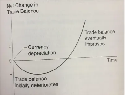
This mechanism is present in equilibrating expected asset returns, as found in the uncovered interest rate parity condition. This indicates a negative relationship between the domestic interest rate and the spot exchange rate, holding the foreign interest rate and the expected future exchange rate as constant. On the other hand, a positive relationship between interest rates and exchange rates can result from the effect of exchange rates on aggregate demand. A higher exchange rate leads to an increase to a country’s trade balance (Shapiro, 1991).
12
Fig. 1. The Theoretical J-Curve adapted from Shapiro (1991).
In Cavallo and Ribba (2014), the presence of different stationary variables, the convergence of national inflation rates and the euro-area inflation rate require the inflation differential to be a stationary variable. More precisely, a systemic, desirable property for a currency area is that the different national rates would gravitate around the European Monetary Union (EMU) average inflation.
PPP states that exchange-adjusted price levels should be identical worldwide. Hence, a unit of the HC should have the same purchasing power around the world. This idea is linked to the LOP, but it must be reformulated in such a way that accounts for transportation and transaction costs between countries, since they are positive. Arbitrage may be too costly because of transportation costs, and the prices of the item could change during transportation. Such price changes could lead to an absence of an inflation differential, and if the local government were to intervene, it could consequently cause the disequilibrium of the exchange rate. These factors explain why the PPP might not hold (Karl Persson, 2008).
2.2. Empirical results regarding the relation among
interest, exchange and inflation rates
13
According to Ida Bache (2006), there are two broad categories of tests with respect to PPP. The first group tries to test the LOP by comparing prices of individual goods across countries. This test was used on a case study made by Haskel and Wolf (2001), who found that deviations from the LOP are large are persistent. Moreover, those deviations reflect changes in nominal exchange rates. The second group tests relative PPP by observing if the real exchange rate is susceptible to converging on a constant value as time progresses (i.e. tests of unit roots in the real exchange rate).
Nonetheless, the earliest test, which relates to a study made by Frenkel (1981) rejected the PPP hypothesis, except in hyperinflating economies, as the failures of exchange rate models may be attributed to assume incorrectly that PPP is accurate. It is hard to measure the relationship between nominal exchange rate and relative prices, even if the price indices are calculated with strict standards. The results suggest that PPP does not hold continuously (Taylor, 1995).
Rogoff (1996) summarised the famous PPP puzzle as follows: if the exchange rate can be so volatile in the short term, why does it take such a long time for it to converge on the exchange rate predicted by PPP? A number of empirical studies have documented that exchange rate behaviour can be well captured by the smooth transition autoregressive (STAR) model from Granger and Teräsvlrta (1993).
Cumby (1997) studied Big Mac parity, which is based on PPP, to investigate exchange rates across different currencies and how they should be adapted in order to have identical costs for a specific basket of goods. Furthermore, he argues that if adjustments towards parity take place through exchange rates, then Big Mac parity may be helpful in forecasting exchange rate changes. The focus of the study was based on Rogoff’s dilemma: reconciling large, short-term deviations from parity with slow deviations back to parity.
In a recent paper, Altissimo, Benigno and Palenzuela (2011) study the underlying factors of inflation differentials in a currency area. In an empirical sense, they find two main results: persistent inflation differentials affect the euro area and the different responses of Eurozone countries to euro-area shocks play a pre-eminent role in explaining the evolution of the inflation differentials.
2.2.2. Why is purchasing power parity considered empirically
imperfect?
14
Taylor (2000) points out that several studies support the relative PPP hypothesis, since the deviations from PPP are extremely volatile and large in the short term. Most findings lean in the direction of Rogoff’s (1996), since the deviations in PPP seem to disappear. The short-term volatility of real exchange rates can be reconciled with the slow rate, as short-term exchange rate volatility points to financial and monetary shocks.
What could be the flaws of PPP? As mentioned previously, there are
transportation costs, tariffs and taxes to be paid as well as external information and technology. This border effect is illustrated by Rogers and Jenkins (1995), who revealed that identical goods at different locations are different economic objects and that the specifications of each location are essential to know. The variations in the prices for similar goods across borders appear to be far more significant in explaining real exchange rates than the movements in the relative prices of different goods within a country’s borders are. Engel and Rogers (1996) conclude that when markets are segmented, price discrimination can occur.
Nominal exchange rates can fluctuate without influencing each other, resulting in a wedge between the prices for domestic and foreign goods. Eventually, this leads to imperfect competition in the market, because better conditions are required for foreign companies to invest in another country for the balance between demand and supply to be near the conditions of equilibrium.
2.3. Exchange, interest and inflation rates after the euro
Exchange rate movements might affect inflation in the euro area. The exchange rate can influence euro-area inflation both directly via the price of imported final consumer goods and indirectly via the price of imported intermediate goods used in euro-area domestic production.
In general, fluctuations of or adjustments to price levels cannot keep pace with the change of economic structure, which will shock the exchange rate. Therefore, PPP cannot be an accurate predictor of real exchange rate, since the international movements caused by economic structural change influence the exchange rate.
Devaluation, in its turn, calls for inflation. In fact, as foreign firms tend to lose market share in the euro area following a depreciation of the euro, they must keep their prices as stable as possible. The euro’s depreciation translates into higher
15
production costs due to more expensive imported inputs with an inflationary impact on domestic consumer prices.
The European Union is built on the idea of a single market defined as an area without frontiers in which the free movement of goods, persons, services and capital is ensured. However, this policy leaves the rest of the world at a disadvantage in relation to these conditions, as the economic conditions and politics of European countries are made in a way where the balance of exports and imports outside of Europe is more restrictive than they are from Europe to other countries.
Cardão-Pito (2017) notes that rating agencies’ failures are consistent with
Reinhart and Rogoff’s (2009) claim that sovereign ratings are not good indicators of the likelihood of banking and/or sovereign crises. These countries’ current accounts showed yearly deficits, with imports being systematically higher than exports (Lane, 2012; Mirdala, 2015). At the beginning of the euro currency system, the Greek and Italian banking sectors did not show any signs of bubbles. Eventually, banks were pushed into crisis by systematically funding government budget deficits.
The two basic features of the European monetary system (EMS) were the
exchange rate mechanism (ERM) and the European currency unit (ECU). The ECU was a composite currency through which all member states’ currencies were represented in different quantities.
As Emerson et al. (1992) note, the independence and autonomy of the European Central Bank is, in a way, a structure in which a stable and credible monetary regime requires an independent central bank to guarantee price stability. Until 2008, the European economy did not have many risks, as the Monetary Union still worked, although it had its limitations. The Central Bank defined the interest rates both in the short term and in the long term. The crisis came to reveal that since the banks are not the same the risks and economies are not the same, and a bank crisis could result in a sovereign crisis where the government has to intervene. Usually in this situation, there would be a transfer of risk from the financial sector to the public sector.
In 2005, Ludger Linneman performed a study, in which he stated that a higher real interest rate with a balanced government budget commands a higher tax rate since it implies higher interest payments on the existing stock of debt and because reduced demand diminishes the tax base. He made the following three points:
(i) the inflation response to higher interest rates is increasing;
(ii) the consumption response is decreasing in the steady-state
16
(iii) for standard parameters, with debt-to-output levels observed in many
European countries, a nominal interest rate increase can even increase inflation.
Forward-looking variables, including market expectations of macroeconomic indicators, are likely to contain relevant information about future movements in the yield curve. Core inflation has been generally considered the appropriate operational target. This measure has been stable and has been a good indicator of underlying (long-term) inflation, particularly in developed economies. By expressing aggregate inflation as a weighted average of the inflations of these two sectors and varying the weight of flexible-price inflation, we consider the inflation measure to be a policy variable.
The fundamental equilibrium exchange rate is defined as the real effective exchange rate value that is compatible with macroeconomic equilibrium. The fundamental equilibrium exchange rate is sometimes referred to as a way that estimates the real effective exchange rate equilibrium. fundamental equilibrium exchange rate (FEER) shows that the value of the exchange rate that is the result of current account assets or deficits, which in turn is appropriate for the long-term structural inflow of the capital or economy outflow, assumes that the country does not have restrictions to trade freely and is trying to attain internal balance. FEER focuses on a theory of exchange rate determination that predicts the future evolution of the exchange rate, as it calculates the medium-term real effective value of a currency in order to assess the current value of the exchange rate. In the behavioural equilibrium exchange rate (BEER), the previous concept is absent, as the relevant notion of equilibrium is the value given by an appropriate set of explanatory variables.
FEER internal balance is identified as the level of output consistent with both full employment and a low, sustainable rate of inflation. The external balance is characterised by the flow of resources between countries. This model uses the core of the macroeconomic balance approach, as this is the identity equating the current account (𝐶𝐴) to the negative of the capital account (𝐾𝐴) (𝐶𝐴 = −𝐾𝐴). The equilibrium relationship between the current and capital accounts is given by the equation:
𝐶𝐴 = 𝑏0 + 𝑏1𝑞 + 𝑏2𝑦̅𝑑 + 𝑏3𝑦̅𝑓 = −KA Where 𝑞 is the real effective exchange rate;
𝑦̅𝑑 is the function of home demand;
17 𝑏1 < 0, 𝑏2 < 0 and 𝑏3 > 0
If we solve the previous equation for 𝑞, we obtain the FEER as: 𝐹𝐸𝐸𝑅 = (−KA − 𝑏0 − 𝑏2𝑦̅𝑑 − 𝑏3𝑦̅𝑓)/ 𝑏1
The FEER is a method to calculate a real exchange rate that is consistent with medium-term macroeconomic equilibrium.
The BEER is an alternative to FEER and is represented by the equation: 𝑞𝑡 = 𝛽1′𝑍1𝑡 + 𝛽2′ 𝑍2𝑡 + 𝜏′𝑇𝑡 + 𝑡
Where 𝑍1 is a vector of economic fundamentals that are expected to have persistent effects over the long term;
𝑍2 is a vector of economic fundamentals that affect the real exchange rate over the medium term, which may coincide with the business cycle;
𝛽1 and 𝛽2 are vectors of reduced-form coefficients;
𝑇 is a vector of transitory factors affecting the real exchange rate in the short term;
𝜏 is a vector of reduced-form coefficients; and 𝑡 is a random disturbance term.
The current equilibrium rate 𝑞′, which is different from the real exchange rate, is the level of the exchange rate given by the current values of the two sets of economic fundamentals:
𝑞𝑡′ = 𝛽1′𝑍1𝑡 + 𝛽2′ 𝑍2𝑡
This model is recursive, as the capital account has an impact on both the current and long-term equilibrium exchange rate. The real exchange rate and the real interest rate adjust so that the current account balance is willingly financed by wealth holders. Goldman Sachs (1996, 1997) published a work regarding these methods, and their results appear to support the presumption of the BEER approach that the real exchange rate is related to economic fundamentals.
According to Cardão-Pito’s research, the expressions PIGS (Portugal, Ireland, Greece and Spain) or PIIGS (adding Italy to the previous list) were conveyed in
18
academic texts (e.g. Cheng, Wu, Lee & Chang 2014; Fernandes & Mota, 2011; Gärtner, Griesbach & Jung, 2011) and popular media, such as the Financial Times and
Economist (BBC, 2010). One thing these countries have had in common is that they
integrated the European single-currency project, the euro, and experienced some form of crisis after integration. Although their economic frameworks, characteristics and performances were quite different, to some extent, they were victims of economic imbalances and institutional shocks due to a poorly structured monetary integration process.
Fig. A.4. displays the GDP growth rate from 1999–2014. In this figure, there are two different periods. One is from 2008 onwards, where the five countries previously referenced had years of economic contraction, or very poor economic growth. However, from 1999–2007, their situations were quite distinct. Portugal and Italy experienced modest GDP growth. Since a significant part of banks’ assets are real estate loans (Saunder, Cornett, & McGraw, 2006), banks can be greatly disturbed by shocks in real estate markets. Among the five countries, only Italy had a relatively small current account deficit in 2007.
After the crises, national states again became relevant, and some devolved into self-fulfilling spirals of capital outflows and interest rate increases (Canale, 2015). The five countries and their banks’ abilities to obtain funding from foreign financial institutions consequently degraded. Financial markets placed further pressure on these countries (Barbosa & Costa, 2010; De Haas & Van Horen, 2012; Gärtner et al., 2011; Lane, 2012). Fig. A.5. illustrates the worsening of the countries’ ten-year debt yields. From 1999–2007, the euro operated as a single currency, showing similar spreads and variations of only a few points among euro-area countries (including Germany). After 2008, however, the spreads became quite larger for the five aforementioned countries, especially Greece. Due to negative consequences and shocks from the crises, these countries’ populations were put through some extreme measures that, to some extent, amounted to internal defaults (Cardao-Pito & Baptista, 2015).
Reinhart and Rogoff (2009, 169-170) compared banking crises in different countries and concluded that a banking crisis increases the probability that a country will default on their internal or external creditors.
Portugal is an example of the impact of an unnatural number of banking crises. From 1945 to 2007, Portugal had no banking crises, while the European average was 1.4 banking crises per country (Reinhart and Rogoff, 2009). After 2007, Portugal registered several occurrences of a banking crisis, which may explain the difficulty it faced in meeting the expectations and obligations of its creditors. Adopting the euro may explain this, as Portugal also adopted a market where the
19
exchange rate was absent among countries using the ECU, reducing the real interest rates and financial spreads for Portuguese banks and corporations. As a result of adopting the euro, major Portuguese banks began borrowing money from financial institutions abroad and pumping enormous liquid assets into the Portuguese economy. Eventually, the Portuguese government intervened demanding public funds, leading to a large increase in the national sovereign debt, which increased external and internal defaults (Cardão-Pito & Baptista, 2016).
In agreement with Cardão-Pito & Diogo Baptista (2016), there may be limitations for Portugal that result from adopting the euro. They are the mutation of the Portuguese banking system into a market-based banking system, a lack of adequate European regulations and institutions to implement the euro project and the behaviour of euro-area financial institutions that might have provided high risk loans to Portuguese banks.
In political economics, countries are classified into one of three categories based on their financial systems: government-led credit-based, bank credit-based and capital market-based (Zysman 1983; Hall and Soskice 2001). However, many countries have observed recent mutations, making them no longer classifiable in the traditional typology of capitalism, as these countries rely on what has been called a market-based banking system, which was the case in Portugal (see for instance, Hardie et al. 2013; Hardie and Howarth 2013a).
3. Research question, data and
methodology
3.1. Problem
This research aims at observing the relation that exists between the key variables of PPP: inflation rate, interest rate and exchange rate. In the context of the euro, the exchange rate was set as fixed for participating countries, but the other two variables were not. Backus and Smith (1992) tested the real business cycle (RBC) model:
20 𝑑𝑆 𝑆 = 𝜂 [( 𝑑𝐶1 𝐶1 −𝑑Π1 Π1 ) − (𝑑𝐶2 𝐶2 −𝑑Π2 Π2 )] +𝑑Π1 Π1 −𝑑Π2 Π2 . (1)
To study the relation 𝑌(𝑡) = 𝐴𝑋(𝑡) , Phillips and Loretan (1991) developed an equation with non-linear relations with additional leads and lags empirically,
𝑌(𝑡) = 𝐴𝑋(𝑡) + 𝑎+1[𝑌(𝑡 + 1) − 𝐴𝑋(𝑡 + 1)] + 𝑎−1[𝑌(𝑡 − 1) − 𝐴𝑋(𝑡 − 1)]
+ 𝑏−1[𝑋(𝑡) − 𝑋(𝑡 − 1)] + 𝑐−1[𝑌(𝑡) − 𝑌(𝑡 − 1)] + 𝑒(𝑡) (2)
3.1.1 Inflation Rate
Inflation measures variation in the prices of goods and services. When inflation is negative, there is deflation, which means the prices of goods have decreased. In this thesis, inflation is measured through the consumer price index (CPI). This indicator assesses a basket of goods and services that are representative of a country’s population. As the prices of these goods will change through time, this allows the researcher to verify the annual price variations, or the country’s inflation rate.
3.1.2 Interest Rate
The interest rate is the load of money that the borrower will pay to the granter. The interest rate is the quota at which the interest is indemnified. The mathematical estimation models consider the variable as being positive, which originate issues in the current economic direction. One way that a central bank has to drop the value of the currency is to depreciate its interest rate as stated by Frankena (2016).
3.1.3 Exchange Rate
The exchange rate is the price at which a country’s currency can be converted into another country’s currency. The nominal exchange rate (NER) is the price of one currency in terms of another, and it is also known as the domestic price of the foreign currency. The real exchange rate (RER) between two currencies is the product of the NER and the ratio of prices between two countries with different currencies, like the yen and the euro following Carbonari (2009) approach.
21
3.1.4 Nominal and real exchange rate differences
This sub-section explains the differences between RER and NER. Each seems essential to test the PPP theory. They provide a comprehensive overview of the rate of currency exchange between two countries. RER and NER are important variables to understand in order to compare the costs of living between countries with different currencies or with the same currency. The NER defines the value of a given currency that can be traded for a single unit of another. The RER shows the amount of goods or services in a given country that can be exchanged for a single unit of that good or service in a different country. In this study, the NER is considered equal to one in every year for every country, as it is only studied using the euro.
3.2. Tests for PPP
This section demonstrates the empirical proposition regarding the PPP by observing the relationship between inflation, interest and exchange rates; although as mentioned before, the exchange rate is a fixed variable, since it is constant through time as this study deals solely with the euro. Annual data on ten-year bond yields are representative of the interest rate, and the inflation rate is the dependent variable. Real GDP, nominal GDP, government gross debt and trade balance (i.e. exports less imports) are the control variables for the period from 1999–2016 for twelve OECD countries (Austria, Belgium, Finland, France, Germany, Greece, Ireland, Italy, Luxembourg, Netherlands, Portugal and Spain). The previous data were taken from the Eurostat, Bloomberg and Ameco databases.
3.2.1. Multicollinearity
As mentioned by Verbeek [25], multicollinearity is when a linear relationship among explanatory variables leads to unreliable regression estimates. To illustrate this, consider the variance of the ordinary least squares (OLS) estimator of a single
coefficient 𝛽𝑘 in a multiple regression framework with an intercept as follows:
𝑉𝑎𝑟(𝛽𝑘) = 𝜎 2 1 − 𝑅𝑘2 1 𝑁[ 1 𝑁∑(𝑥𝑖𝑘− 𝑥̅𝑘) 2 𝑁 𝑖=1 ] −1 , 𝑘 = 2, … , 𝐾,
22
Where 𝑅𝑘2 is the squared multiple correlation coefficient between 𝑥
𝑖𝑘 and the
other independent variables.
There is a way to detect multicollinearity through the variance inflation factor (VIF):
𝑉𝐼𝐹(𝑏𝑘) = 1
1 − 𝑅𝑘2
It indicates the variance of 𝑏𝑘 is inflated compared with the hypothetical
situation when there is no correlation between 𝑥𝑖𝑘 and any other independent
variable.
3.2.2. Test for unit roots in dynamic panels
Here the properties of the three kinds of panel unit root tests proposed respectively by LL, IPS and MW are presented. Those tests are based on the following regression, which allows for fixed effects and unit-specific time trends:
𝛥𝑦𝑖𝑡 = 𝛾𝑖 + 𝛿𝑖𝑡 +𝜃𝑡 + 𝜌𝑖𝑦𝑖𝑡−1 +𝜁𝑖𝑡, = 1,2,.. 𝑁, 𝑡 = 1, 2, …, 𝑇.
Where the error term is 𝜁𝑖𝑡~(0,𝜎2);
[𝜁𝑖𝑡𝜁𝑗𝑠] = 0 ⩝ 𝑡, 𝑠 and 𝑖 ≠ 𝑗; and
𝜃𝑡 is the common time effects.
The error term can allow heteroscedasticity and some dependence in the
error terms of each unit. The null hypothesis of interest for all three tests is 𝐻0: 𝜌𝑖 =
0 ⩝ 𝑖. The tests allow for different degrees of heterogeneity of 𝜌𝑖 under the alternative
hypothesis if 𝑦𝑖𝑡 is stationary. One of the possible problems when analysing the time
series on a number of countries simultaneously is heterogeneity, as it is natural that the model parameters for each country differ. Robertson and Symons (1992) and Pesaran and Smith (1995) mention the importance of heterogeneity in dynamic panel data models and observe the biases that may arise, as they may destroy the relationships between individual series.
Levin and Lin (1992) argue the alternative hypothesis is the case where the
23
3.2.3. Stationary stochastic process
A stochastic process is stationary if its mean is constant over time, its variance is constant over time and its covariance is constant between two periods. A stochastic process is said to be strictly stationary if its properties are unaffected by a change of time origin, meaning that the joint probability distribution at any set of
times 𝑡1, 𝑡2, … , 𝑡𝑚 must be the same as the joint probability distribution at times 𝑡1+
𝑘, 𝑡2+ 𝑘, … , 𝑡𝑚+ 𝑘. As mentioned before, it must satisfy the following:
→ (𝑥1) = 𝐸(𝑥2) = ⋯ = 𝐸(𝑥𝑇) = 𝐸(𝑥𝑡) = µ,
and
→ 𝑉𝑎𝑟(𝑥1) = 𝑉𝑎𝑟(𝑥2) = ⋯ = 𝑉𝑎𝑟(𝑥𝑇) = 𝑉𝑎𝑟(𝑥𝑡) = 𝜎2𝑥,
→ 𝐶𝑜𝑣(𝑥1, 𝑥1+ 𝑘) = 𝐶𝑜𝑣(𝑥2, 𝑥2+ 𝑘) = ⋯ = 𝐶𝑜𝑣(𝑥𝑇− 𝑘, 𝑥𝑇) = 𝐶𝑜𝑣(𝑥𝑡, 𝑥𝑡− 𝑘)
This means that the assumption implies the auto covariance
𝛾𝑘 = 𝐶𝑜𝑣(𝑥𝑡, 𝑥𝑡− 𝑘) = 𝐸[(𝑥𝑡− µ), (𝑥𝑡− 𝑘 − µ)]
And the autocorrelations
𝜌𝑘 = 𝐶𝑜𝑣(𝑥𝑡, 𝑥𝑡− 𝑘)
[𝑉𝑎𝑟(𝑥𝑡). 𝑉𝑎𝑟(𝑥𝑡−𝑘)]12
=𝛾𝑘
𝛾0
3.2.4. Cointegration
Let 𝑋𝑡 = (𝑋1𝑡 𝑋2𝑡)′ be two I(1) variables, such that 𝑋1𝑡 and 𝑋2𝑡 contain
stochastic trends.
Cointegration occurs if the stochastic trends in 𝑋1𝑡 and 𝑋2𝑡 are the same such
that they cancel, which is also known as a common trend. Furthermore, if 𝑋1𝑡 and 𝑋2𝑡
cointegrate, then the deviation 𝑢𝑡 = 𝑋1𝑡 − µ − 𝛽2𝑋2𝑡 is a stationary process with a mean
24
The Engel and Granger approach becomes relevant to understand that cointegration requires a combination of the variables to be stationary. Consider the equilibrium demand for money equation:
𝑚𝑡 − 𝑝𝑡 = 𝛽1 + 𝛽2𝑦𝑡 + 𝛽3𝑟𝑡 + 𝑡,
Where 𝑚 is money demand, 𝑝 is the price level, 𝑦 is the real income and 𝑟 is the interest rate. It is required that 𝛽2 > 0 and 𝛽3 < 0.
(i) The linear transformation of any process keeps its order of
integration:
𝑥𝑡~(0) ⇒ 𝛼 + 𝛽𝑥𝑡 = 𝑧𝑡~𝐼(0); 𝑦𝑡~𝐼(1) ⇒ 𝛼 + 𝛽𝑦𝑡 = 𝑝𝑡~𝐼(1)
(ii) If both 𝑥𝑡 and 𝑦𝑡 are stationary, then the combination of these two
processes is a stochastic process
𝑥𝑡~(0), 𝑦𝑡~𝐼(0) ⇒ 𝛼𝑥𝑡 + 𝛽𝑦𝑡 = 𝑧𝑡~𝐼(1)
(iii) The linear combination between a stochastic process and a process of
a degree equal to one results in an integrated process with a degree of one (i.e. 𝐼(1) is a dominant property)
𝑥𝑡~(0), 𝑦𝑡~𝐼(1) ⇒ 𝛼𝑥𝑡 + 𝛽𝑦𝑡 = 𝑧𝑡~𝐼(1)
(iv) The combination of two processes of order one is an order one process
𝑥𝑡~(1), 𝑦𝑡~𝐼(1) ⇒ 𝛼𝑥𝑡 + 𝛽𝑦𝑡 = 𝑧𝑡~𝐼(1)
(v) The combination of two processes of order one is an order one process
𝑥𝑡~(1), 𝑦𝑡~𝐼(1) ⇒ 𝛼𝑥𝑡 + 𝛽𝑦𝑡 = 𝑧𝑡~𝐼(1)
(vi) There are some exceptions to the previous conditions, as the linear
combination may be (0). So, 𝑥 and 𝑦 are cointegrated (i.e. there is a stationary equilibrium between these two variables)
𝑥𝑡~(1), 𝑦𝑡~𝐼(1) ⇒ 𝛼𝑥𝑡 + 𝛽𝑦𝑡 = 𝑧𝑡~𝐼(0)
25
Following Hamilton’s (1994) approach, consider the OLS estimation of a Gaussian (1) process,
𝑦𝑡 = 𝑝𝑦𝑡−1+ 𝑢𝑡 𝑡 = 1, … , 𝑛
Where 𝑢𝑡~i.i.d. (0, 𝜎2), and 𝑦0 = 0.
From the previous information, certain properties according to Stock (1987) follow:
(i) When the variables are cointegrated, then the estimator is consistent.
(ii) When using finite samples, the skewness of the estimator may be
significative, as the expected value may not coincide with the true values of the parameters, which makes the study of cointegration for short periods of time difficult.
(iii) The OLS estimator is not asymptotically efficient.
(iv) Generally, the asymptotic distribution theory is not valid.
3.3.2. Test for Cointegration
McCoskey and Kao (1998) propose the use of the average of the augmented Dickey-Fuller (ADF) statistics over cross-sections, based on Im et al. (1997), to test the hypothesis that no cointegration exists in heterogeneous panels.
First consider two time series 𝑥1𝑡 and𝑥2𝑡, which are both I(1), meaning that each
series has a unit root. If the two series cointegrate, than the coefficients are µ and 𝛽2
such that
𝑥1𝑡 = µ + 𝛽2𝑥2𝑡+ 𝑢𝑡
By using the Engle-Granger approach, first the series would need to be tested for their unit roots. If both are I(1), than the defined regression equation must be run and the residuals must be saved, as these must be tested for a unit root. If the null hypothesis for the residuals is rejected, than the hypothesis of the two variables cointegrating cannot be rejected.
26
If one of the series is stationary (i.e. I[0]) and the other is I(1), they cannot be cointegrated since cointegration implies that they share common stochastic trends and that a linear relationship between them is stationary since the stochastic trends will cancel and thereby produce a stationary relationship.
So, the steps that should be followed using dynamic OLS are:
1. Select the optimal lag of leads and lags using information criteria;
2. Estimate the equation by OLS and test whether the residuals are I(0) or I(1) according to the ADF test. If the residuals are I(0), the variables are cointegrated.
4. PPP and cointegration: The euro
case
4.1. The approach employed
In order to use the nominal GDP and real GDP as one variable, the GDP deflator was used to make a division between the first variable and the second. Furthermore, the trade balance was calculated using exports and imports, as previously mentioned. The logarithm was then applied to all variables. The reason for the existence of the previous variable is due to its correlation with respect to the inflation rate.
Here the NER is dropped due to its statistical characteristics. Therefore, for each of the countries in the euro area, there are two variables considered dependent, one of which is the inflation rate. The other variable is the interest rate, which corresponds to the annual yields on ten-year bonds.
There are two types of tests that are presented in this paper. The first uses
the variables of the studied twelve countries as panel data. The second studies each country individually in order to understand the relationship between the dependent and independent variables and observe differences in their behaviour between countries.
27
4.2. Panel unit root testing
The panel unit root has been tested with the joint null hypothesis of a unit root for each country. Some issues when doing panel data tests are cross-sectional dependence, heterogeneity in dynamics and error-term properties. So, this section presents the basic statistics for each dependent variable and its histogram, but only for LOG_INFLATON_RATE and LOG_INTEREST_RATE, as NER is a vector with equal values in every entry; hence, it has no variance and therefore no relation with the previous variables. This is done for the panel data and the countries separately. These can be seen in the tables below.
The unit root test was conducted for inflation rate and interest rate. As explained before, the purpose of this test is to check the null hypothesis that there is unit root data or that the data are not stationary. Thus, in the statistical package, the unit root test has been applied to check whether the data is stationary. It can be seen in the tables, in relation to the unit root test for the countries, that none of the countries have a stationary inflation rate variable. Furthermore, some countries, like Belgium, do not have this variable as stationary, which should not happen due to the relation between inflation, interest and exchange rates.
The interest rate in the case of Ireland is not stationary, which should also not happen. This means that the relationship between the previous two variables is not the same in the countries and that the panel data test cannot correctly present the stationarity for each country.
28
Table 4.2.1. Results of unit root tests for the panel data and euro-area countries from Austria to Greece
Variables Methods Statistics values Conclusion Statistics values Conclusion Statistics values Conclusion Statistics values Conclusion Statistics values Conclusion Statistics values Conclusion -5.425*** -4.355*** Not -2.240 Not -6.588*** -4.795*** -5.070*** (0.000) (0.004) stationary (0.200) stationary (0.000) (0.002) (0.001) -5.488*** -4.531* Not -2.260 Not -4.025** -4.951*** -5.043*** (0.002) (0.011) stationary (0.430) stationary (0.034) (0.006) (0.005) -5.616*** -1.016 Not -1.231 Not -6.759*** -4.916*** -5.128*** (0.000) (0.264) stationary (0.191) stationary (0.000) (0.000) (0.000) -5.331*** -5.360*** -4.837*** -5.648*** -5.487*** -3.538* (0.000) (0.000) (0.001) (0.000) (0.000) (0.021) -5.331*** -5.337*** -4.816*** -5.642*** -4.515** -3.404* (0.003) (0.003) (0.007) (0.001) (0.014) (0.088) -3.976*** -4.538*** -3.501*** -4.270*** -4.044*** -3.676* (0.000) (0.000) (0.001) (0.000) (0.000) (0.000) Germany I(1)*** I(1)*** I(1)*** France I(1)** I(1)** I(1)** Greece I(1)*** I(1)*** I(1)*** Austria
Augmented Dickey-Fuller (intercept)
Augmented Dickey-Fuller (trend and intercept)
ADF - Fisher Chi-square
I(1)***
I(1)***
I(1)*** Augmented Dickey-Fuller (no trend and no intercept)
Finland Belgium I(1)* I(1)* I(1)* Inflation rate Interest rate
Augmented Dickey-Fuller (intercept)
Augmented Dickey-Fuller (trend and intercept)
Augmented Dickey-Fuller (no trend and no intercept)
Levin, Lin & Chu t*
Im, Pesaran and Shin W-stat
ADF - Fisher Chi-square
PP - Fisher Chi-square Levin, Lin & Chu t*
Im, Pesaran and Shin W-stat
PP - Fisher Chi-square I(1)*** I(1)*** I(1)*** I(1)*** I(1)*** I(1)*** I(1)*** I(1)*** I(1)*** I(1)** I(1)** I(1)** I(1)*** I(1)*** I(1)***
29
Table 4.2.2. Results of unit root tests for the panel data and euro-area countries from Ireland to Spain
Variables Methods Statistics values Conclusion Statistics values Conclusion Statistics values Conclusion Statistics values Conclusion Statistics values Conclusion Statistics values Conclusion Statistics values Conclusion -4.013** -4.860** -6.442*** -5.564*** -4.773** -6.138*** (0.009) (0.001) (0.000) (0.000) (0.002) (0.000) -3.842** -3.828** -6.328*** -5.566*** -4.601** -6.131*** (0.043) (0.047) (0.000) (0.002) (0.013) (0.000) -3.965** -4.902** -6.519*** -5.712*** -4.316** -6.100*** (0.000) (0.000) (0.000) (0.000) (0.000) (0.000) -4.653*** (0.000) -3.317*** (0.000) 49.261*** (0.001) 50.522*** (0.001) -2.922 Not -4.083 -5.200*** -5.292*** -6.092*** -4.551* (0.064) stationary (0.007) (0.001) (0.000) (0.000) (0.003) -2.908 Not -3.990 -4.996*** -5.288*** -5.858*** -3.819* (0.185) stationary (0.032) (0.006) (0.003) (0.001) (0.054) -2.944 Not -4.024 -5.395*** -3.956*** -6.319*** -4.723* (0.006) stationary (0.000) (0.000) (0.000) (0.000) (0.000) -13.202*** (0.000) -10.367*** (0.000) 131.415*** (0.000) 139.946*** (0.000) Ireland I(1)** I(1)** I(1)** Augmented Dickey-Fuller (intercept)
Augmented Dickey-Fuller (trend and intercept)
ADF - Fisher Chi-square
Augmented Dickey-Fuller (no trend and no intercept)
I(1)*** I(1)*** I(1)*** Spain I(1)*** I(1)*** I(1)*** Portugal I(1)** I(1)** I(1)** Luxembourg I(1)*** I(1)*** I(1)*** Netherlands I(2)*** I(2)*** I(2)*** Italy I(1)** Inflation rate Interest rate
Augmented Dickey-Fuller (intercept) Augmented Dickey-Fuller (trend and intercept) Augmented Dickey-Fuller (no trend and no intercept)
Levin, Lin & Chu t* Im, Pesaran and Shin W-stat
ADF - Fisher Chi-square PP - Fisher Chi-square
Levin, Lin & Chu t* Im, Pesaran and Shin W-stat
PP - Fisher Chi-square I(1)*** I(1)*** I(0)*** I(2)* I(2)* I(2)*** I(1)*** I(1)*** I(1)** I(1)** I(1)** I(0)*** Panel Data I(0)*** I(0)*** I(1)*** I(1)*** I(1)*** I(2)*** I(2)*** I(2)* I(1)** I(1)**
30
4.3. Cointegration Testing
A cointegrating relationship requires the variables to be at least integrated at order one, I(1). To carry out a cointegration analysis, it is necessary to conduct a unit root test to see if the time series are in fact I(1). Afterwards, it is possible to conduct a cointegration test on the relevant series. One of the most popular tests is Johansen’s trace test/maximum eigenvalue test. This test is required to work with every variable. Therefore, in this section, the variables LOG_INFLATION_RATE is the
dependent variable and LOG_INTEREST_RATE, LOG_DEFLATOR_GDP,
LOG_GOVERNMENT_GROSS_DEBT and LOG_TRADE_BALANCE are independent variables for the panel data, as it is not possible to do this for every country. It is only required to test cointegration for one variable as dependent, since this test is directly related to the stationarity of each variable. Hence, if the dependent variable is I(2) and one of the independent variables is I(1) and the linear relation is I(1) then cointegration is confirmed.
First, the Pedroni residual cointegration test was computed for the previous
variables. It tested 𝐻0: there is no cointegration in this model. There is no
deterministic trend in the panel cointegration. There are two scenarios that are
presented: 𝐻1 within-dimension and between-dimension, with four different
statistics for each scenario. For the v-stat and rho-stat, we accept 𝐻0, and for the
PP-stat and ADF-PP-stat, we reject 𝐻0 and accept 𝐻1, meaning the variables are
cointegrated. As most of the p-values are significant in eleven tests, 𝐻1 is accepted.
Therefore, the five variables are cointegrated; they have a long-term association. Next, the results are checked for a deterministic trend in individual intercepts and trends. It can be seen that out of eleven outcomes, six are significant for all
significance levels. So, 𝐻1 is accepted, meaning that the variables are cointegrated
for this trend.
Finally, the no intercept or trend option is checked. Six out of eleven
probabilities are significant, so the majority of the p-values reject 𝐻0. Hence, the
variables are cointegrated. All the tests conclude that the variables are cointegrated. Then, the Kao residual cointegration test is checked. The probability of ADF
is less than 1%, so 𝐻0 is rejected for all levels of significance. Thus, the five variables
31
Table 4.3.1. Results of residual cointegration tests for all variables
Deterministic trend specification
Statistics values no trend intercept and trend no intercept or trend Kao Conclusion Panel v-Statistic 0.108 -1.251 0.262 No Cointegration
(0.456) (0.894) (0.396)
Panel rho-Statistic 0.731 1.674 -0.396 No Cointegration
(0.767) (0.953) (0.346)
Panel PP-Statistic -5.750*** -6.989*** -4.603*** Cointegration
(0.000) (0.000) (0.000)
Panel ADF-Statistic -5.555*** -6.907*** -5.006*** Cointegration
(0.000) (0.000) (0.000)
Panel v-Statistic (Weighted) -0.984 -2.520 -0.436 No Cointegration
(0.837) (0.994) (0.669)
Panel rho-Statistic (Weighted) 0.799 1.699 -0.269 No Cointegration
(0.788) (0.955) (0.394)
Panel PP-Statistic (Weighted) -6.946*** -7.561*** -5.276*** Cointegration
(0.000) (0.000) (0.000)
Panel ADF-Statistic (Weighted) -6.725*** -7.125*** -5.584*** Cointegration
(0.000) (0.000) (0.000)
Group rho-Statistic 2.136 2.899 0.824 No Cointegration
(0.983) (0.998) (0.795)
Group PP-Statistic -10.211*** 9.840*** -6.753*** Cointegration
(0.000) (0.000) (0.000)
Group ADF-Statistic -6.904*** -7.138*** -6.924*** Cointegration
(0.000) (0.000) (0.000) ADF -6.721*** Cointegration (0.000)
32
4.4. Estimating Equation
This development consists of working the panel data using the pooled OLS regression model, fixed effect or Least Squares Dummy Variable (LSDV) model and the random effect model. As there are two dependent variables, it was run in two ways: one with the interest rate as the dependent variable and one with inflation rate as the dependent variable.
The first model pooled all the observations together and ran the regression model, neglecting the cross-section and the time series nature of the data. The major problem with this model is that it denies the heterogeneity that may exist among the countries.
The second model allows for heterogeneity among the countries by allowing it to have its own intercept value. The fixed effect is due to the fact that although the intercept may differ across the countries, it does not vary over time (i.e. it is time invariant).
Finally, in the third model, the countries have a common mean value for the intercept.
After running the above three models, the best model to accept was
determined using the Hausman test, where 𝐻0 is the random-effects model.
Hence, for the inflation rate variable, the pooled regression model concluded that LOG_GOVERNMENT_GROSS_DEBT and LOG_TRADE_BALANCE are significant variables to explain LOG_INFLATION_RATE for all significance levels. In this case, the fixed effect model was run after the correlated random effects–Hausman test. However, when using LOG_INTEREST_RATE as a dependent variable, LOG_INFLATION_RATE and LOG_DEFLATOR_GDP are significant variables to explain the variable at a significance level of 5%. Here, the random effects model is accepted according to the Hausman test. The first two tables illustrate the panel data
33
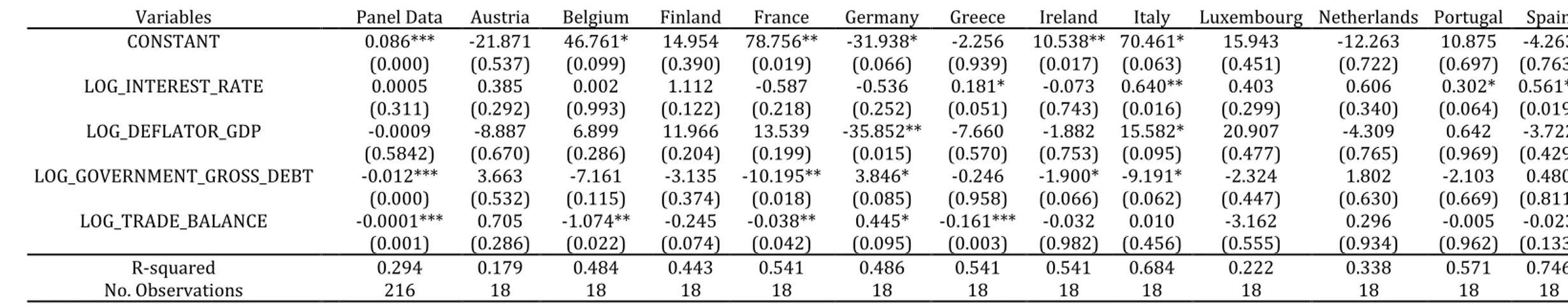
Table 4.4.1. Regression results for LOG_INFLATION_RATE as a dependent variable
Variables Panel Data Austria Belgium Finland France Germany Greece Ireland Italy Luxembourg Netherlands Portugal Spain CONSTANT 0.086*** -21.871 46.761* 14.954 78.756** -31.938* -2.256 10.538** 70.461* 15.943 -12.263 10.875 -4.263 (0.000) (0.537) (0.099) (0.390) (0.019) (0.066) (0.939) (0.017) (0.063) (0.451) (0.722) (0.697) (0.763) LOG_INTEREST_RATE 0.0005 0.385 0.002 1.112 -0.587 -0.536 0.181* -0.073 0.640** 0.403 0.606 0.302* 0.561** (0.311) (0.292) (0.993) (0.122) (0.218) (0.252) (0.051) (0.743) (0.016) (0.299) (0.340) (0.064) (0.019) LOG_DEFLATOR_GDP -0.0009 -8.887 6.899 11.966 13.539 -35.852** -7.660 -1.882 15.582* 20.907 -4.309 0.642 -3.722 (0.5842) (0.670) (0.286) (0.204) (0.199) (0.015) (0.570) (0.753) (0.095) (0.477) (0.765) (0.969) (0.429) LOG_GOVERNMENT_GROSS_DEBT -0.012*** 3.663 -7.161 -3.135 -10.195** 3.846* -0.246 -1.900* -9.191* -2.324 1.802 -2.103 0.480 (0.000) (0.532) (0.115) (0.374) (0.018) (0.085) (0.958) (0.066) (0.062) (0.447) (0.630) (0.669) (0.811) LOG_TRADE_BALANCE -0.0001*** 0.705 -1.074** -0.245 -0.038** 0.445* -0.161*** -0.032 0.010 -3.162 0.296 -0.005 -0.023 (0.001) (0.286) (0.022) (0.074) (0.042) (0.095) (0.003) (0.982) (0.456) (0.555) (0.934) (0.962) (0.133) R-squared 0.294 0.179 0.484 0.443 0.541 0.486 0.541 0.541 0.684 0.222 0.338 0.571 0.746 No. Observations 216 18 18 18 18 18 18 18 18 18 18 18 18
Standard errors are reported in parentheses. *, **, *** indicates significance at the 90%,
34
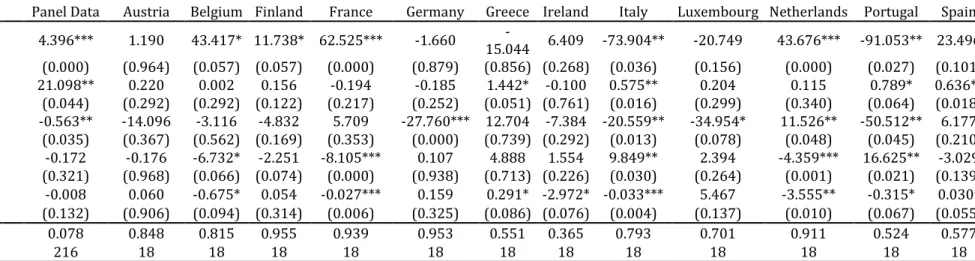
Table 4.4.2. Regression results for LOG_INTEREST_RATE as a dependent variable
Variables Panel Data Austria Belgium Finland France Germany Greece Ireland Italy Luxembourg Netherlands Portugal Spain CONSTANT 4.396*** 1.190 43.417* 11.738* 62.525*** -1.660 15.044 - 6.409 -73.904** -20.749 43.676*** -91.053** 23.496 (0.000) (0.964) (0.057) (0.057) (0.000) (0.879) (0.856) (0.268) (0.036) (0.156) (0.000) (0.027) (0.101) LOG_INFLATION_RATE 21.098** 0.220 0.002 0.156 -0.194 -0.185 1.442* -0.100 0.575** 0.204 0.115 0.789* 0.636** (0.044) (0.292) (0.292) (0.122) (0.217) (0.252) (0.051) (0.761) (0.016) (0.299) (0.340) (0.064) (0.018) LOG_DEFLATOR_GDP -0.563** -14.096 -3.116 -4.832 5.709 -27.760*** 12.704 -7.384 -20.559** -34.954* 11.526** -50.512** 6.177 (0.035) (0.367) (0.562) (0.169) (0.353) (0.000) (0.739) (0.292) (0.013) (0.078) (0.048) (0.045) (0.210) LOG_GOVERNMENT_GROSS_DEBT -0.172 -0.176 -6.732* -2.251 -8.105*** 0.107 4.888 1.554 9.849** 2.394 -4.359*** 16.625** -3.029 (0.321) (0.968) (0.066) (0.074) (0.000) (0.938) (0.713) (0.226) (0.030) (0.264) (0.001) (0.021) (0.139) LOG_TRADE_BALANCE -0.008 0.060 -0.675* 0.054 -0.027*** 0.159 0.291* -2.972* -0.033*** 5.467 -3.555** -0.315* 0.030* (0.132) (0.906) (0.094) (0.314) (0.006) (0.325) (0.086) (0.076) (0.004) (0.137) (0.010) (0.067) (0.055) R-squared 0.078 0.848 0.815 0.955 0.939 0.953 0.551 0.365 0.793 0.701 0.911 0.524 0.577 No. Observations 216 18 18 18 18 18 18 18 18 18 18 18 18
Standard errors are reported in parentheses. *, **, *** indicates significance at the 90%,
35
4.5. Covariance and Correlation matrices
The relationships between variables are well represented in covariance and correlation matrices, as covariance measures the joint variability between random variables and correlation (i.e. the statistical relationship regarding the dependence for variables). Covariance, unlike correlation, is not constrained to being between -1 and 1. Therefore, the matrices of covariance and correlation between the two variables LOG_INFLATION_RATE and LOG_INTEREST_RATE are presented below:
Panel Data Austria Belgium Finland France Germany Greece Ireland Italy Luxembourg Netherlands Portugal Spain
Correlation between LOG_INFLATION RATE and LOG_INTEREST_RATE 0.222 0.105 0.338 0.285 0.440 0.247 -0.166 0.066 0.746 0.427 0.567 0.369 0.645 Covariance between LOG_INFLATION RATE and LOG_INTEREST_RATE 0.006 0.120 0.488 0.446 0.492 0.279 -1.182 0.249 0.932 0.835 0.980 1.102 1.142
Standard errors are reported in parentheses. *, **, *** indicates significance at the 90%,
95%, and 99% level, respectively
Matrix 4.5.1. Table of covariances and correlations between LOG_INFLATION RATE and LOG_INTEREST_RATE
36
4.6. Panel DOLS model
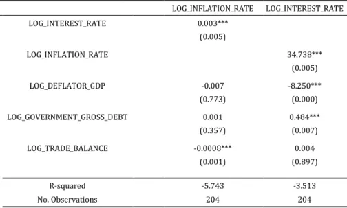
There are some conditions to test the panel cointegration using Eviews. First, the variables must be stationary on the same order. Then, if and only if a variable is cointegrated, the DOLS model is applied to the panel data for long-term relationships. Thus, all of the variables available are used: LOG_INFLATION_RATE, LOG_INTEREST_RATE, LOG_DEFLATOR_GDP, LOG_GOVERNMENT_GROSS_DEBT and LOG_TRADE_BALANCE.
A cointegration regression is conducted for all variables with LOG_INFLATION_RATE as the dependent variable and no trend specification with the DOLS method or group panel method. As the p-values are less than 1% for LOG_INTEREST_RATE and LOG_TRADE_BALANCE, this means that for
LOG_INFLATION_RATE, the previous variables are significant.
LOG_TRADE_BALANCE has a negative association with LOG_INFLATION_RATE, and LOG_INTEREST_RATE has a positive association with LOG_INFLATION_RATE. This can be seen in Table 4.6.1 with LOG_INTEREST_RATE and LOG_INFLATION_RATE as dependent variables in each case.
Dependent Variable LOG_INFLATION_RATE LOG_INTEREST_RATE LOG_INTEREST_RATE 0.003*** (0.005) LOG_INFLATION_RATE 34.738*** (0.005) LOG_DEFLATOR_GDP -0.007 -8.250*** (0.773) (0.000) LOG_GOVERNMENT_GROSS_DEBT 0.001 0.484*** (0.357) (0.007) LOG_TRADE_BALANCE -0.0008*** 0.004 (0.001) (0.897) R-squared -5.743 -3.513 No. Observations 204 204 Standard errors are reported in
parentheses. *, **, *** indicates significance at the 90%, 95%, and 99% level, respectively
37
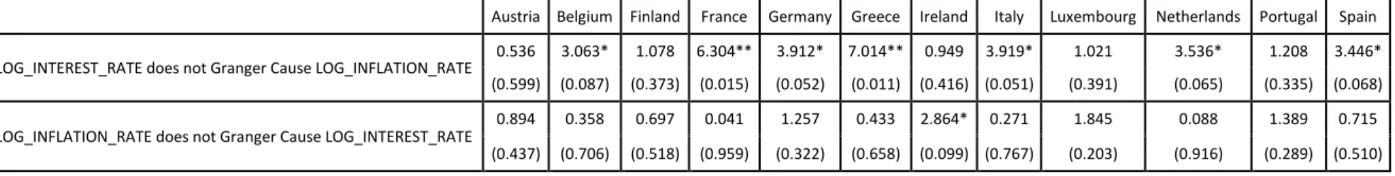
4.7. Pairwise Granger Causality
This causality test is closely related to the idea of cause and effect, although it is not exactly the same. For instance, a variable X is causal to variable Y if X is the cause of Y or Y is the cause of X. The objective of the test is to know if a particular variable comes before another in a time series. In other words, Granger causality does not indicate a causal link. The null hypothesis for the test is that lagged x-values do not explain the variation in y. This test was conducted for each of the countries presented below:
Table 4.7.1. Results of pairwise Granger causality test for the variables LOG_INFLATION_RATE and
LOG_INTEREST_RATE
Austria Belgium Finland France Germany Greece Ireland Italy Luxembourg Netherlands Portugal Spain
LOG_INTEREST_RATE does not Granger Cause LOG_INFLATION_RATE 0.536 3.063* 1.078 6.304** 3.912* 7.014** 0.949 3.919* 1.021 3.536* 1.208 3.446* (0.599) (0.087) (0.373) (0.015) (0.052) (0.011) (0.416) (0.051) (0.391) (0.065) (0.335) (0.068)
LOG_INFLATION_RATE does not Granger Cause LOG_INTEREST_RATE
0.894 0.358 0.697 0.041 1.257 0.433 2.864* 0.271 1.845 0.088 1.389 0.715 (0.437) (0.706) (0.518) (0.959) (0.322) (0.658) (0.099) (0.767) (0.203) (0.916) (0.289) (0.510)
Standard errors are reported in parentheses. *, **, *** indicates significance at the 90%,
38
5. Findings and their limitations
5.1. Summary of findings
The Phillips-Perron (1988) unit root test was the first regression model by OLS to be tested. Thus, whether the model has a unit root is checked, and the null hypothesis
(𝐻0: there is unit root) is rejected if the series is not stationary. From Tables 4.2.1 and
4.2.2, it can be concluded that the inflation rate is stationary on level and the interest
rate is stationary after first difference. For the cointegration test, Table 4.3.1 shows the results. According to Johansen (1992), if all of the tests suggest that the variables are cointegrated, then cointegration between the variables is confirmed.
In addition, it is necessary to estimate the equation from each country in order to understand the importance of the variables for each country, respectively. The results can be seen in Tables 4.4.1 and 4.4.2 using LOG_INFLATION_RATE and LOG_INTEREST_RATE, which verify that between these two variables there are similar results for each country (and panel data); however, when crossing the information, significant differences from the estimation can be seen (e.g. Germany and Greece). This should not happen, as PPP theory would mean that all the countries should have identical results since the relationship of the two previous variables should be equivalent. The correlation and covariance is a good example of the previous summary, as there are several discrepancies between the correlation and covariance of LOG_INFLATION_RATE and LOG_INTEREST_RATE, as France has a positive covariance and correlation, but Greece has a negative covariance and correlation. This means that the relationship between the previous variables varies. From the panel DOLS model, it can be concluded that significant variables with p-values at a less than 10% significance level means that the error correction term is statistically significant in affecting the short-term dynamic. Hence, the results show that interest rate is affected by inflation rate, GDP and gross debt, whereas inflation rate is affected by interest rate and trade balance.
Finally, the causality test concluded that, in general, inflation rate is not causal to interest rate, though some countries’ (i.e. Belgium, France, Germany, Greece, Italy, Netherlands and Spain) data rejected the null hypothesis, meaning that for these cases, interest rates may explain the variation in inflation rate.
39
5.2. Limitations
During the research, in order to test the PPP theory for euro-area countries, some difficulties arose. The theory itself does not consider that there are non-identical products between countries; therefore, some products may not be tradable. Additionally, the sample was small one, as only twelve out of nineteen cases had all the information required; the countries that were not present in the study had information missing. Indeed, this happened due to the absence of these countries from the euro area during the introduction of the euro as a currency. As referred to previously, the short period of study could be a limitation of this research. Finally, the biggest issue for this study was that it was not possible to reproduce previous studies (e.g. USD\EUR and USD\GBP).
6. Conclusion
The objectives of this paper are emphasized once again to see if the expectations were met and to raise relevant questions on this topic. The theory of PPP, in line with Mackinnon as stated by Taylor (1988), says:
Until a more robust theory replaces it, I shall assume that purchasing power parity among tradeable goods tends to hold in the long run in the absence of overt impediments to trade among countries with convertible currencies.
This theory was studied with econometric models. The first step was to obtain variables through known platforms including Bloomberg, Eurostat and Ameco. Next, the exchange rate in this case is a time series equal to one in every entry for every country, meaning that the euro in country 𝑖 has the same value as in country 𝑗. This was a problem when trying to conduct a regression and the tests for stationarity and cointegration, as the variable of exchange rate could not enter the study for reasons of multicollinearity.
Therefore, the variables had to be tested as described in chapter four. The results are described in chapter five. As explained previously, the results did not support the theory, as the behaviours of the variables over time with respect to each country were not similar. They should have been similar, since the exchange rate was equal to one in this case for all countries, which was the main variable in this study. This is a reason to refute the PPP theory’s application in the euro area.
In comparison to previous studies of PPP with different approaches, the relationship between exchange, inflation and interest rates differs depending on the