Intra-Annual land cover mapping: Automatic training sample extraction from old maps for intra-annual land cover mapping at central of Portugal

William Alexander Martínez Blanco

INTRA-ANNUAL LAND COVER MAPPING

AUTOMATIC TRAINING SAMPLE EXTRACTION FROM

OLD MAPS FOR INTRA-ANNUAL LAND COVER MAPPING

AT CENTRAL OF PORTUGAL

Aut o matic Trai ning Samp le ext rac tion Fr om Ol d Ma ps for Intr a -annual Land Cove r Ma ppi n g at Cent ral of Po rtu gal W illia m Alex an de r M ar tín ez B lanco

Intra-annual land cover mapping

Automatic Training Sample Extraction From

Old Maps for Intra-annual Land Cover Mapping

at Central of Portugal.

Dissertation supervised by Dr. Mario Caetano

Professor, Nova Information Management School University of Nova Lisbon, Portugal

Dr. Edzer Pebesma

Professor, Institute for Geoinformatics University of M¨unster, Germany

Dr. Jorge Mateu

Professor, Department of Mathematics University of Jaume I Castell´on, Spain

Acknowledgment

I want to thank the three supervisors for their contributions which have greatly improved the original version of this thesis. Moreover, I must express my especial gratitude to professor Mario Caetano, for the patient guidance, encouragement and advice he has provided throughout the time frame of this thesis. His office was always open whenever I had a question about my research or writing.

I would also like to thank all the members of staff at DGT and Professors at Nova IMS who helped me in my supervisor’s absence. Especially, I would like to thank Daria Ludtke, Inˆes Gir˜ao and Hugo Costa, and professors Marco Painho and Joel Silva for the suggestions they made in reference to Chapter 4 of this work.

I also leave my most sincere gratitude to the Erasmus Mundus Master pro-gram Science in Geospatial technologies, headed by the professors Marco Painho, Christoph Brox, Christian Kray, Joaqun Huerta and Michael Gould. I am very honored for having been one of the recipients of this Erasmus scholarship.

Last but not least, I want to thank all my family who has always supported me unconditionally in every endeavor that I have undertaken in my life. With seven and a half thousand of kilometers away from them, I do not imagine this journey without their calls and constant motivation.

Abstract

Automatic Training Sample extraction From

Old Maps for Intra-annual Land Cover Mapping

at Central of Portugal.

Making operational efficient the production of Land Use Land cover (LULC) mapping over large areas as the consistency and accuracy keep a high quality is an essential condition for the implementation of applications that require pe-riodic information, such as forest fire propagation, crop monitoring or climate models. The increasing spatial and temporal resolution satellite images, such as those provided by Sentinel 2, open new opportunities for producing accurate datasets that can improve the lack of production of global and regional LULC maps with fine scale and up-to-date information. In this context, while this the-sis aimed to make automatic the generation of intra-annual maps implementing a workflow that consists of supervised classification in synergy with automatic extraction of training samples from an old map, it also aimed to use singular and BAP composites. Therefore, after a preliminary selection and preprocessing of the implemented spectral bands in the classification both from single and BAP composites of Sentinel 2 images of 2017, a random selection of training points is extracted from an old reference map; national LULC map of Portugal, COS 2015. We performed a classification scheme using support vector machine (SVM) and Random forest (RF) classifiers with two datasets of six and nine different number of land cover classes. The out-of-date information derived from the old map led us to evaluate the viability of implementing two refining procedures over the data

Abstract

to improve accuracy; one based on margins of NDVI signals and another based on an iterative learning procedure. Since the proposed methodologies did not lead to improving OA on the classification of any of the images of 2017, we questioned for robustness of the classifiers RF and SVM by injecting different levels of noise during the modeling. Finally, the free cloud and phenological maximization of the BAP composites become in a consistent and efficient input for the production of seasonal LULC mapping.

Keywords

Best available pixel

Intra-annual Land Use Land Cover

Support vector machine and random forest

Acronyms

DGT - Dire¸c˜ao-Geral de Ordenamento do Territ´orio, Portugal

COS Uso e Ocupa¸c˜ao do Solo

L1C Level-1C

L2A Level-2A

MMU Minimum Mapping Unit

SVM Support vector machine

RF Random forest

LCLU Land Cover Land Use

BAP Best available pixel

NIR Near Infrared

Index Of Figures

3.1 Study area . . . 16

3.2 Available images Sentinel 2, 2017 . . . 17

3.3 COS Map 2015, Nomenclature Level 1 . . . 18

3.4 Class definition of the two datasets and COS nomenclature 2015 . 20 3.5 Distribution of the number of samples of the external dataset per percentage . . . 21

4.1 General Methodology . . . 24

4.2 Methodology image preprocessing . . . 25

4.3 Methodology composites . . . 26

4.4 Methodology selection points from old map. . . 26

4.5 Methodology extraction features from images. . . 27

4.6 A visualization of the splits of the training dataset during classifi-cation . . . 28

4.7 NDVI signals over time for classes of trees . . . 29

4.8 Iterative learning procedure to define informativeness based on boosting and the measurement of information entropy . . . 31

5.1 Spatial distribution of the training data. . . 34

5.2 Baseline July 25 2015, RF classifier . . . 35

5.3 Level of importance variables random forest . . . 36

5.4 Perfomance classifiers RF and SVM, scene-based composites 2017 37 5.5 pixel-based composite Spring. . . 39

5.6 Performance of the classifications, single images vs BPA compos-ites, 9 classes classification . . . 40

Index Of Figures

5.7 Performance of the classifications, single images vs BPA

compos-ites, 6 classes classification . . . 40

5.8 Normalized confusion matrix, classification scene-based composite July 29 . . . 41

5.9 Seasonal mapping. . . 43

5.10 NDVI signal for herbaceous classes . . . 44

5.11 Traning data distribution after applying NDVI rules . . . 45

5.12 Cleaning processing NDVI, Performance over scene-based compos-ites 2017 . . . 46

5.13 Informativeness score for herbaceous . . . 47

5.14 Example of low informative sample for sealed . . . 47

5.15 Cleaning preprocessing using batch learning, Image July 29 2017 . 48 5.16 Cleaning preprocessing using batch learning per class, Image July 29 2017 . . . 50

5.17 Performance of the proposed methodology over a traning data with 30% of noise, scene-based composite July 29 . . . 50

5.18 Performance random forest vs SVM using COS data under different levels of noise, scene-based composite July 29 . . . 51

5.19 Sensitivy analysis parameters random forest . . . 52

5.20 Sensitivy analysis parameters SVM with RBF kernel . . . 53

1 accumulative values of precipitation per month, 2015. Source data: netCDF files NOAA . . . 63

2 Intersection of the classes of COS map 2015 with the study area, Nomenclature based on recent recommendation from EEA on Coper-nicus land monitoring services . . . 64

3 Intersection of nine classes of COS map 2015 with the study area, Nomenclature based on recent recommendation from EEA on Coper-nicus land monitoring services . . . 65

Index Of Tables

5.1 Accuracy assessment 9 classes . . . 42 5.2 Accuracy assessment 6 classes . . . 42

Index Of The Text

1.1 Problem statement and Motivation . . . 1

1.2 Objectives . . . 4

1.2.1 Research question . . . 4

1.2.2 Aim . . . 4

1.2.3 Objectives . . . 4

2 Literature Review 7 2.1 Land cover mapping and image classification . . . 7

2.2 Best pixel available . . . 8

2.3 Automatic selection and refinement of training data . . . 9

2.4 Classification algorithms and tunning parameters . . . 10

2.4.1 Support vector machines . . . 11

2.4.2 Random forest . . . 12

2.5 Accuracy assessment in land cover classification . . . 12

3 Data and study area 15 3.1 Study area . . . 15

Index Of The Text 3.3 COS map . . . 17 3.4 External dataset . . . 19 4 Methodology 23 4.1 Image preprocessing . . . 23 4.2 Seasonal Composites . . . 25

4.3 Automatic training data from a old map . . . 26

4.4 Classification schema . . . 27

4.5 Filtering training data . . . 28

4.5.1 Trimming NDVI signals . . . 29

4.5.2 Filtering training data based on a iterative learning procedure 30 4.6 Evaluation of the robustness of the classifiers . . . 30

5 Results 33 5.1 Automatic training selection from COS map . . . 33

5.2 Classification . . . 34

5.2.1 Baseline . . . 35

5.2.2 Classification using RF and SVM (images 2017) . . . 36

5.3 Single maps vs seasonal maps . . . 37

5.4 Filtering training data . . . 42

5.4.1 Trimming NDVI signals . . . 42

5.4.2 Filtering training data using a iterative learning procedure 46 5.5 Robustness of SVM and RF . . . 50

5.5.1 Effect estimation of the hyper-parameters with Noise in the train data . . . 51 6 Conclusions 55 6.1 Recommendations . . . 56 Bibliographic References 57 Annexes 63 xvi

1 Introduction

1.1 Problem statement and Motivation

Characterizing land use land cover (LULC) over large areas is a fundamental task in any environmental, cultural and political study since it provides a base-line for governments to undertake and monitor policies that look for sustainable livelihoods in harmony with the ecosystems. Remote sensing in synergy with image processing makes possible the identification and mapping of the land cover system, and then, the assessment and monitoring of the resources at different temporal and spatial scales (Rogan and Chen, 2004). After almost four decades of earth observation and development of powerful algorithms in mapping LULC, the research continues adapting new approaches that lead to its update to be operationally efficient and benefit from the massive data available through new technology with open data policy (G´omez et al., 2016).

The recent operation of the satellites Sentinel 2A and 2B of the European Union’s Earth observation program Copernicus can play a crucial role in the new and future generation of LULC maps (G´omez et al., 2016). With an increase of the revisit frequency and better spatial resolution imagery -as never before- the research can improve the lack of production of global and regional LULC maps with a fine scale and up-to-date information. In this context, the availability of intra-annual maps can be central in a broad spectrum of applications such as forest fire propagation (Navarro et al.,2017), crop monitoring (Vuolo et al.,2018), inundation mapping (Kordelas et al.,2018), and climate change models(Radoux et al., 2014). However, increasing the continuity in time of the characterization of the land cover system over large areas by using this new technology can also

1 Introduction

lead to new operational challenges. Specifically, in making operationally efficient its production while its consistency and accuracy keeps high quality. (Radoux et al.(2014),Bontemps et al. (2016)).

Traditionally, remote sensing image classification is an automatic approach of making LULC mapping where the level of human intervention may vary de-pending on the classification procedure (Rogan and Chen (2004),Inglada et al. (2017)). In this context, unsupervised procedures (K means, SOM) are attractive for an automatic definition of classes boundaries in comparison with supervised classifiers (RF, SVM, Maximum likelihood) that require the construction of train-ing data (Mather and Tso, 2016). However, in the context of classification over large areas, high dimensionality and fast reproduction, unsupervised methods can lose effectiveness due to the time-consuming post-processing and complexity in the interpretation of clusters (Chen and Gong, 2013). Therefore, the better ex-perience with supervised classification over large areas with high dimensionality (Khatami et al. (2016), Colditz et al. (2011)) raise the question if an automatic collection of training labels can overcome its drawback of needing reference data for its implementation.

The availability of previous maps in the study area represents an essential reference (Colditz et al.,2011), and therefore an effective method for automation of collecting training data. However, even though they can represent a rich source of information, this data may contain no informative labels that can hinder the results in the classification (Pelletier et al., 2017b). In this context, predefined labels by the old maps can be contributive to the classification of one recent image or not depending on different factors. For example, point random extraction can intersect complexities of a wide diversity of classes that were simplified in one class in the map or intersect outdated labels.

Support Vector Machine (SVM) and Random Forest (RF) represent state of the art algorithms for its application in the production of LULC (Thanh Noi and Kappas, 2018); important for their ability to handle high dimensionality, being superior to unsupervised approaches and being insensitive to overfitting (Bishop, 2006). Although these methods are also known for being resistant to anomaly

1.1 Problem statement and Motivation

data, a classifier trained in a set of large amount of wrong labels can turn out in a wrong model (Pelletier et al., 2017a). Therefore, this thesis aims to refine the sampling by exploring the viability of implementing two cleaning procedures; one based on margins of NDVI signal and other based on an iterative learning procedure that uses boosting and the measurement of information entropy to control quality data.

While exploring the advantages to work with old maps as reference data for the classification of Sentinel 2 imagery, this thesis also aims to evaluate the con-sistency and effectiveness of the production of BAP composites as input in the production on intra -annual LULC mapping over large areas. Since the high revisit frequency of Sentinel 2 does not guarantee free-cloud imagery, BAP ap-proach can reproduce imagery without cloud contamination (White et al., 2014). BAP composites have been developed by using different kind of protocols, which mainly depend on the use of NDVI values and distances to the masked clouds (Hermosilla et al.,2015). In this context, based on experiments of Holben(1986) with VHRR time series. That is, making composites by maximizing the NDVI per pixel in an arrange of several scenes in order to capture the state of the vegetation when is more photosynthetically active, we propose to make seasonal composites as a case of study.

Therefore, the proposed classification procedures are tested on Sentinel-2 im-ages acquired in 2017. The training data is extracted from COS map of Portugal 2015 (Caetano et al., 2015) (Uso e Ocupa¸c˜ao do Solo), whereas the validation corresponds to two datasets, one out-of-date that corresponds to a fraction of the dataset 2015 and another constructed using satellite image interpretation in 2017.

1 Introduction

1.2 Objectives

1.2.1 Research question

This thesis formulated the following research question:

• How useful is the integration of training sampling extracted from old maps for an automatic production of intra-annual land cover mapping?

1.2.2 Aim

To answer the research question we defined that the main objective of this thesis is:

• To evaluate the performance of the integration of training samples extracted from old maps in a supervised classification schema for the production of intra-annual mapping.

1.2.3 Objectives

In order to achieve the formulated general aim, this thesis proposed the following specific objectives:

• To evaluate the performance of RF and SVM in the classification of Sentinel 2 images 2017 using training data extracted from the national LULC map of Portugal COS 2015?

• To evaluate the usability of COS map 2015 in the automation of the clas-sification of Sentinel 2 imagery in 2017.

• To explore the viability of implementing a refining procedure of mislabeled data from ol maps based on margins of NDVI signals, and an iterative batch learning procedure that can lead to an improvement of the performance of image classification.

• To evaluate the consistent and efficiency of the BAP composites in the production of intra-annual LULC mapping over large areas?

1.2 Objectives

Finally, this thesis had a focus on processing Sentinel 2 data products in Python and R. Readers interested in the used scripts to achieve the above objec-tives can visit the following link in GitHub .

2 Literature Review

This Chapter will provide an overview of the literature relevant for the study. The topics covered are land cover mapping and image classification in Chapter 2.1, Best pixel available composites in Chapter 2.2, automatic selection and refinement of training data for supervised classification in Chapter 2.3, and the basis of the implemented classification algorithms in this study in Chapter 2.4.

2.1 Land cover mapping and image classification

The synergy of earth observation and image processing has made possible the monitoring and identification of the land cover system at a global and regional scale (Rogan and Chen,2004). Despite the early experience of thematic mapping with Sentinel 2 imagery (data from 2015), it has shown potential in a different number of applications. Specifically, in the production of a new generation of land cover maps that consider fine regional scale and up to date information (Kordelas et al. (2018),Vuolo et al. (2018),Navarro et al. (2017)).

Traditionally, global and regional LULC mapping uses image classification to identify and monitor the land cover system automatically (Rogan and Chen, 2004). From this angle, the task of image classification can be seen from the per-spective of clustering cases by their relative spectral similarity (i.e., unsupervised) or in the localization of cases that match predefined classes that have been char-acterized spectrally (i.e., supervised). Unsupervised algorithms (SOM, K-means) uses the spectral information derived by the satellite to define clusters. Since the clusters do not necessarily reflect the data classes under analysis, the product pass by post-processing in order to merge the clusters with specific homogeneous

2 Literature Review

variance (Wang and Feng, 2011). Increasing the dimensionality both in features and area of analysis can turn out in a time-consuming and not effective opera-tional task due to the post-processing and the complexity in the interpretation of the clusters (Vesanto et al., 2000). Alternatively, supervised classifiers (SVM, RF, Maximum Likelihood) labels the pixels according to their similarity of sam-ples labeled a priori using reference data (Mather and Tso,2016). The quality of the reference data is determinant since they must represent the problem exten-sively; otherwise, the classifier is unable to generalize the problem to unseen pixels (Bousquet et al., 2004). The task of collecting data is usually time-consuming since it is collected manually. Although the accumulation of databases to perform semiautomatic classification, the data that come from the reference map is not error free. This experience can lead to poor results and biased classification (Pal and Mather, 2006).

Besides the experience of classification in LULC mapping according to the basis of the training process, the classifiers can also be categorized on the bases of theoretical models (parametric and not parametric). The primary appeal of using nonparametric models (RF, SVM) in comparison with parametric (ML) is based on its free assumptions of distributions and its high flexibility for adapting to different kind of variables (Mather and Tso, 2016). However, its application depends strictly on the quality and volume of the data (Pal and Mather, 2006).

So far, we have briefly introduced the image classification as a usual method in the production of land cover mapping. Therefore, besides giving particular interest to the classifiers and quality of data, in the next Chapter, we will make a parenthesis in order to talk about the quality of the imagery in the classification.

2.2 Best pixel available

The approach of pixel-based composites provides the means to reproduce cloud-free and phenological consistent image composites (G´omez et al., 2016). Com-posites have been developed by using several kinds of protocols, which mainly depend on the use of NDVI values and distances to the masked clouds to define

2.3 Automatic selection and refinement of training data

the best available pixel(BAP) (Hermosilla et al., 2015). The first examples of this approach obey to applications in the 80s using AVHRR and MODIS im-ages (Holben, 1986). Primarily, the methods were based on maximizing NDVI or minimizing view angle to select the best observation for a given pixel within a specified compositing period. The limitations derived by the fact of the coarse spatial resolution of sensors that accounted for high temporal resolution. How-ever, with the opening of Landsat and Sentinel 2 archive, the generation of BAP composites has become technically feasible. New attempts for the selection of the best pixel aim at implementing several rules respect distance to the clouds and including different kind of sensors at the same time. For example, a scoring protocol proposed in White et al. (2014) that seek to weight every pixel of the time series of images according to their proximity to the clouds, date of analysis and type of sensor.

2.3 Automatic selection and refinement of training

data

Since the task of collecting data manually for the process of classification is usually time - consuming, the strategy to obtain it automatically resides in the idea of extracting labels of available databases or old maps (Inglada et al., 2017). However, the use of that reference data can be constrained by two different reasons as discussed in Pelletier et al. (2017b) and Radoux et al. (2014). On the one hand, the gap between the time production of the map and the date of the image acquisition can turn out in out-up-date labels. On the other hand, effects of spatial continuity in the map can turn out in points retrieving wrong labels in areas of a mixture of classes that were simplified according to the minimum mapping unit of the map. Generally, the presence of this inconsistencies may be not a problem due to the the ability of some classifiers, such as RF and SVM, to deal with anomaly data (Pelletier et al.,2017a). However, the systemic presence of erroneous labels can lead to impact negatively the results of the classification (Tolba, 2010).

2 Literature Review

The operational strategies of removing possible outliers in the training data can be seen from the perspective of exploring the spectral dispersion of the data from different dimensions, or from the perspective of iterative learning procedures (Chandola et al.,2009). On the one hand, distances are crucial in the definition if one point behaves or not like anomaly data. For example, in Radoux et al. (2014) is implemented multiclass border reduction filter (MBRF), where pixels that have the most significant number of neighbors of the same class are inlier for the classification. In other applications such asMeroni et al.(2019),Xu et al. (2016) distances are also crucial; the refining procedures consists of taking out samples that are not within the margins of NDVI signals per class through the year.

On the other hand, the iterative learning procedures consist of integrating to the classification scheme an evaluation of fractions of repetitive misclassified points. In this context, active learning procedures can be roughly divided into online learning and batch learning based techniques (Hazan et al.,2016). In online learning, a classifier selects and adds iteratively samples that are informative for the definition of cluster boundaries (Tuia et al.(2012),Tuia et al. (2009)). While selecting and updating the necessary train data, it takes out not informative data for the classification. However, in the context of batch learning, the approaches define the contrary. That is, while it removes not informative data, it keeps cluster boundaries (B¨uschenfeld and Ostermann (2012),Wu et al. (2004),Pelletier et al. (2017b)).

2.4 Classification algorithms and tunning

parameters

Machine learning algorithms as Random forest and support vector machines are widely used into remote sensing for being able to handle high data dimensionality while being insensitive to over-fitting (Mather and Tso, 2016). In the frame of classification with noise that came from the out-up-date map, RF and SVM can be crucial due to their characteristics of being insensitive to outliers in the

2.4 Classification algorithms and tunning parameters

definition of cluster boundaries. Every classifier has its own type of parameters and versatility to handle different types of data. Defining which one is better than others may depend on the data and the problem domain (Thanh Noi and Kappas(2018),Vuolo et al.(2018)). Therefore, to achieve an optimal classification we will require eventually and optimization of their parameters. In the following two chapters, we will explain which parameters will be optimized and why they matter in the prediction.

2.4.1 Support vector machines

SVM algorithm is a popular supervised classifier that has been widely used in different domains. In the context of remote sensing, it has been extensively used for its good performance (Mountrakis et al.,2011). Particularly, SVM minimizes the error of classification by creating a hyperplane among every set of classes, so that it maximizes the distance between the support vectors of every class. The parameter that controls the margin of the hyperplane is called C and generally as higher its value, the better performance for the training data, but with the risk of losing generalization for unseen data. Conversely, a low value of C will neglect possible outliers in the training data, and thus gaining more versatility to over-fitting.

Since the data may be not linearly separable in the original dimension, the separation is done in a higher spectral space controlled by a kernel. RBF kernel is commonly used for its good results (Shi and Yang(2015),Pelletier et al.(2017a)). However, it requires the optimization of a second parameter, γ, that control the shape of the Gaussian kernel function and thus how much jagged or soft the decision boundary will be. The reason by which eventually an optimization of this parameter will matter is due to high estimations of values of γ; we can turn out with a model that works properly for the training dataset, but losing generalization for unseen data.

2 Literature Review

2.4.2 Random forest

The fundamental idea behind RF is the construction of hundreds of decision trees, considered weak learners, which are then combined to transform them into a strong learner. Its implementation depend on setting up two parameters: number of trees ntree and number of variables randomly sampled as candidates at each split, mtry. In several studies, the default parameters of RF, that is 100 trees and mtry =√p (where p is the number of variables), lead in average to the best performance of the classifier.

According withBreiman(2002), the algorithm works as follows: 1) draw ntree bootstrap samples; 2) For each bootstrap sample, grow and un-pruned tree by choosing best split based on a random sample of mtry predictors at each node; 3) Predict new data using majority votes for classification.

2.5 Accuracy assessment in land cover classification

Generally, the judgment of the quality of LCLU maps depends on the evaluation of the derived map against some ground or reference data for validation. In thematic mapping, the map quality is a function of the degree of correctness of the map that usually is interpreted as accuracy (Foody,2002). Accuracy standards can be diverse, from subjective perspectives as the visual appraisal of the final maps to more objective assessments, such as accuracy metrics based on comparisons of the class labels in the thematic map and ground data. Accuracy may be undertaken for different reasons, such as the general evaluation of the quality of the map or a base for evaluating the performance of different algorithms in the classification (Congalton and Green, 2008).

According to Foody (2002), the confusion matrix is currently the core of the accuracy assessment in the literature. This matrix consists of a cross-tabulation with the percentages of labels correctly classified. The matrix also provides the means to analysis intraclass confusion, so that it may help studies to pay special attention to the performance of the classification over specific classes. Many metrics of classification accuracy can be derived from a confusion matrix (Foody,

2.5 Accuracy assessment in land cover classification

2002). For example, the simple overall accuracy (OA) that determines the total percentage of classes correctly classified; that is, dividing the number of labels correctly classified into the total number of labels. Its simplicity makes it useful for a vast spectrum of applications (Pelletier et al.,2017a). However, in particular, for this thesis, we highlight its importance for working as a base on the comparison of the performance of different algorithms in classification.

In this context, the simplicity of OA may imply its major problem since some users argue that there may be cases where the correct classes were purely classified by chance (Congalton and Green (2008), Pontius (2000)). Therefore, to make a balance of the effects of chance agreement, Cohen’s kappa is proposed. Unlike OA that ranges between 0 and 1, kappa varies between -1 and 1.

3 Data and study area

In this chapter, we introduce the study area and the data to conduct this research. Therefore, In Chapter3.1, we start with the location of the images to classify and the discussion of the interest of developing the methodology in this region. In Chapter 3.2, we introduce relevant technical specifications of the available images during the period of analysis for the classification. To conduct the auto-matic selection of training data we introduce in Chapter 3.3 the old map COS 2015. Finally, in Chapter 3.4, we introduce an external and updated dataset developed by DGT in order to test the results of the proposed methodology.

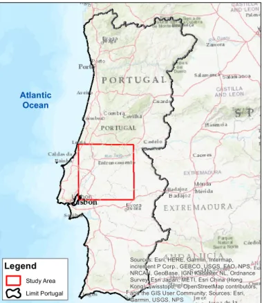
3.1 Study area

We conducted LULC mapping using classification of a series of tiles of Sentinel 2 located at central of Portugal. Figure3.1 shows the location of the study area in red color with a dimension of 100km by 100km. The tiles intersected Tagus river in the region of Santar´em and Vila Franca de Xira at the head of the long narrow estuary.

3.2 Sentinel 2 Imagery

This thesis used Sentinel-2 image time series acquired in 2017. The instruments considers 13 spectral channels in the visible/near infrared (VNIR) and short wave infrared spectral range (SWIR); bands came in 10, 20 and 60 meters resolution. The images were downloaded by using the online system Copernicus Open Access Hub developed by ESA. The imagery was utterly free. An overview of the images

3 Data and study area

Sources: Esri, HERE, Garmin, Intermap, increment P Corp., GEBCO, USGS, FAO, NPS, NRCAN, GeoBase, IGN, Kadaster NL, Ordnance Survey, Esri Japan, METI, Esri China (Hong Kong), swisstopo, © OpenStreetMap contributors, and the GIS User Community; Sources: Esri, Garmin, USGS, NPS Atlantic Ocean Legend Study Area Limit Portugal

Figure 3.1: Study area

under study, the percentage of clouds and the level of the available images are shown in figure 3.2. Data is derived from the S2A and S2B sentinel missions. The lower amount of imagery at the beginning of the year obeys to the release of images from only the first mission; having images every five days was only possible until the second mission S2B was launched on March 2017. Moreover, we distinguish in four colors the imagery used to develop every seasonal composite and in gray color the excluded images; the exclusion of images obeyed to the high cloud contamination of the image (see the percentage of clouds).

The products of Sentinel 2 came in two different levels 1C and 2A. L1C cor-responds to an orthorectification of data using as reference the digital elevation model (PlanetDEM 90). Consequently, a preprocessing is carried to offer mea-surements of reflectance on the top of the atmosphere. Instead, L2A consist of postprocessing of L1C product to provide reflectance measurements on the bot-tom of the atmosphere. In this context, products that came in level 1C ware

3.3 COS map

Day Level Clouds Day Level Clouds Day Level Clouds Day Level Clouds Day Level Clouds

1 Jan 5 1C 60,90% 15 1C 0% 25 1C 28,95% 3 2 Feb 24 1C 21,72% 1 3 Mar 16 1C 54,02% 1 4 Apr 5 2A 0% 15 2A 11,37% 2 5 May 25 2A 2,10% 1 6 Jun 4 2A 0,48% 14 1C/2A 0,30% 2 7 Jul 4 2A 0,22% 9 1C 7,20% 14 2A 0,25% 24 2A 0,25% 29 1C 0,08% 5 8 Aug 3 2A 0,24% 8 1C 0% 13 1C 0% 18 2A 0,13% 23 1C 41,74% 5 9 Sep 2 2A 0% 7 1C 0% 12 2A 0,21% 22 2A 1,65% 27 2A 0% 5 10 Oct 2 2A 0,21% 12 2A 0,19% 22 2A 0,84% 27 2A 0,84% 4 11 Nov 11 2A 0,24% 16 1C 0% 21 2A 0,25% 3 12 Dec 1 2A 2,08% 11 2A 46,31% 16 1C 0,09% 21 2A 0,33% 4 36 Number

Total Number of images Spring Composite Summer Composite Autumn Composite Winter Composite

Figure 3.2: Available images Sentinel 2, 2017

subject of preprocessing using the Sen2Cor processor developed by ESA.

Specifically, the bands used for this project were the following: 10m spatial resolution bands B2 (490nm), B3 (560nm), B4 (665nm), and B8-NIR (842nm), and the 20 m spatial resolution bands B5 (705 nm), B6 (740 nm), B7 (783 nm), B8a (865nm), B11-SWIR (1610nm), and B12-SWIR (2190nm) (ESA, 2017b). The bands Band 9 Water vapour and Band 10 SWIR Cirrus are not part of this study. In this context, the spectral information is mainly characterized by channels in the visible/near-infrared (VNIR) and short wave infrared spectral range (SWIR).

Finally, the 30 meters resolution of the global digital elevation model (DEM) developed by The National Aeronautics and Space Administration (NASA) was used to create the layer of Slope. Therefore, besides of the spectral data provided by Sentinel 2, we also consider the DEM and Slope after considering resampling to the minimum mapping unit (MMU) of analysis.

3.3 COS map

COS map is a national product describing LULC of Portugal with a MMU of 1 Ha and produced using aerial image interpretation. COS map has 5 levels and the level with more detail comprises 48 different classes. DGT is the institute in charge of producing this map and has available four versions (1995, 2007,2010

3 Data and study area

and 2015). Moreover, COS is a composition of polygons, where each polygon represents a homogeneous unity of use and occupation of the soil. Each polygon represents an area of land greater than or equal to the defined MMU of 1 ha, with a maximum distance between lines or equal to 20 m and which percentage of a given class is equal or greater than 75% of the total area.

According to COS 2015, the study area covered a wide variety of land cover types, such as urban fabric (10.1%), agricultural areas (50.1%), water-bodies (1.4%), wetlands (0.1%), forest and semi-natural areas (38%). The landscape shaped by the river and thus an emerge of fertile lands leads to the neighbor communities to set agricultural practices. Therefore, the wide diversity in the agricultural practices and phenology activity corresponded to an desirable sce-nario for conducting this thesis (see figure3.3).

8°0'0"W 8°0'0"W 8°30'0"W 8°30'0"W 9°0'0"W 9°0'0"W 39 °3 0' 0" N 39 °3 0' 0" N 39 °0 '0 "N 39 °0 '0 "N Artificial surfaces Agricultural areas Forest and seminatural areas Water bodies Wetlands Study Area Legend 1.4% 38% 50.1% 10.1% 0.1%

Figure 3.3: COS Map 2015, Nomenclature Level 1

Consequently, the intersection also resulted in 21 different classes with Level 5. This first inspection led to construct table3.4. According to COS nomenclature (pink color), the categories diversifies depending on their level of description. For

3.4 External dataset

example, the agricultural areas comprise 2 categories for level 2: periodic and permanent crops; in this sense, periodic: diversifies in irrigated and not irrigated crops, and permanent: in rice fields, grasslands, vineyard, and olive trees.

Automation of the classification process requires the production of LULC maps with simple nomenclature that allows both an operational replication and a high quality production. Therefore, this thesis proposed to follow recent recom-mendation of European Environmental Agency on Copernicus land monitoring in the future generation of Corine land cover maps (EEA,2018). In this context, we undertook its relation with COS map nomenclature having as a result the gray section in again table 3.4. On the one hand, nomenclature of Dataset 1 matches with the level 1 of nomenclature COS 2015 for the categories of Herbaceous (Agri-cultural areas), sealed surface (Artificial surfaces), water surfaces (water bodies), non vegetation and wetlands (see Figure 2 in Annexes). However, for the spe-cific case of forest and semi-natural areas, dataset 2 diversify the category in 4 subgroups: non-vegetated, shrubs, Coniferous, Eucalyptuses and Holm and Cork trees (see Figure3 in Annexes).

Even though Vinhas and Olivais classes are also part of the intersection of classes in the study area, this thesis do not consider them. Generally, vineyard and olive classes are plantations with fruits. These herbaceous categories have a specific case of sowing in furrows, where the space between them lead to having a mixture of not vegetated and vegetated classes in the pixel. Therefore, since the rest of the categories cover extensively herbaceous class, we did not consider to use them as training data of our models.

3.4 External dataset

Since the presence of anomaly data may be general, both in training and testing, and the cleaning processing is only done over the training, the use of a exter-nal dataset may be fundamental to compare the predictive power of the trained models against test data that reflect correctly the class variation without the exposition to mislabel data due to phenology. In this case, in collaboration with

3 Data and study area

Level 1 Level 2 Level 3 Level 4 Level 5

Shrubs

Vegetação arbustiva e herbácea

Matos Matos Matos

Florestas de pinheiro bravo Florestas de pinheiro

manso Eucalyptus

trees Florestas de eucalipto

Florestas de sobreiro Florestas de azinheira

Arrozais Arrozais Arrozais Pastagens permanentes Pastagens permanentes Pastagens permanentes

Vinhas Vinhas Vinhas

Olivais Olivais Olivais

Planos de água Planos de água Planos de água Planos de água Águas marinhas e costeiras Desembocaduras fluviais Desembocaduras fluviais Desembocaduras fluviais Nomenclature COS 2015 Dataset 2 Dataset 1 Herbaceous Herbaceous

Zonas húmidas Zonas húmidas Zonas húmidas Zonas húmidas Zonas húmidas Planos de água Planos de água Planos de água Cursos de água Cursos de água Cursos de água Planos de água Corpos de água Indústria, comércio e equipamentos gerais Redes viárias e ferroviárias e espaços Tecido urbano contínuo Tecido urbano contínuo Tecido urbano descontínuo Tecido urbano descontínuo Tecido urbano Indústria, comércio e equipamentos gerais Indústria, comércio e equipamentos gerais Redes viárias e ferroviárias e espaços Redes viárias e ferroviárias e Indústria, comércio e transportes Zonas descobertas e com Florestas e meios naturais e semi-naturais Tecido urbano contínuo Tecido urbano descontínuo Territórios artificializados Culturas permanentes Áreas agrícolas e agro-florestais Culturas temporárias de sequeiro e de Culturas temporárias de sequeiro e de Espaços descobertos ou com pouca vegetação Espaços descobertos ou com pouca vegetação Zonas descobertas e com pouca vegetação ou com Florestas Culturas temporárias Culturas temporárias de Florestas de resinosas Florestas de resinosas Florestas de folhosas Florestas de folhosas Water

surfaces Water surfaces

Wetlands Wetlands Woody Sealed surface Coniferous trees Holm and Cork Trees

Non vegetated Non vegetated

Sealed surface

Figure 3.4: Class definition of the two datasets and COS nomenclature 2015

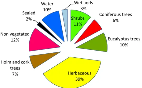
DGT, we had access to an external dataset that corresponds to a satellite image interpretation of 557 random samples using the image of 29 of July of 2017. The distribution of samples is the following: Shrubs: 61, Coniferous trees:35, Euca-lyptus trees: 55, Herbaceous: 217, Holm and cork trees: 38, Non vegetated:69, Sealed: 11, Water:55, Wetlands:16.

3.4 External dataset Shrubs 11% Coniferous trees 6% Eucalyptus trees 10% Herbaceous 39% Holm and cork

trees 7% Non vegetated 12% Sealed 2% Water 10% Wetlands 3%

Figure 3.5: Distribution of the number of samples of the external dataset per percentage

4 Methodology

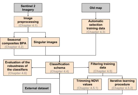
While this thesis aimed to make automatic the production of intra-annual maps implementing a workflow that consisted of supervised classification in synergy with automatic extraction of training samples from an old map, it also aimed to use singular and BAP composites (see Figure4.1). In this context, after a prelim-inary selection and preprocessing of the implemented features in the classification (Chapter 4.1) both from single images and BAP composites (Chapter 4.2), a random selection of training points is extracted from an old map and intersected with the spectral information of the images (Chapter4.3). We performed a clas-sification scheme using SVM and RF classifiers using two datasets with six and nine different number of land cover classes (Chapter4.4). The out-of-date infor-mation derived from the old map led us to evaluate the viability of implementing two refining procedures over the data in order to improve accuracy (Chapter 4.5); one based on margins of NDVI signals and another based on an iterative learning procedure. Besides that, the possible inconsistencies of the labeled data led us to evaluate also the robustness of classifiers RF and SVM by injecting different levels of noise (Chapter 4.6).

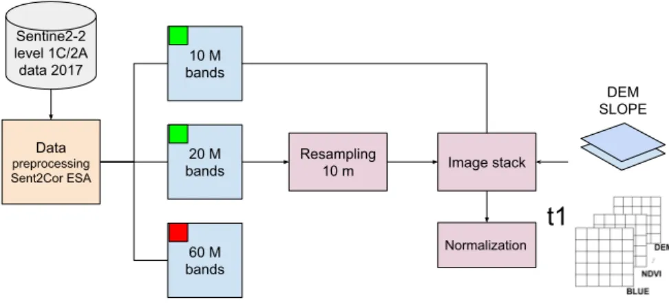
4.1 Image preprocessing

The preprocessing started with the use of Sen2Cor toolbox allowing the conversion of radiance into reflectance. Specifically, this tool provided a product L2A that considered the atmospheric, terrain and cirrus correction of Top-Of- Atmosphere of Level 1C imagery (ESA, 2017). Moreover, the process included the correction of also bands of 60 and 20 meters resolution. However, the objective of this thesis

4 Methodology Image preprocessing (Chapter 4.1) Seasonal composites BPA (Chapter 4.2) Automatic selection training data (Chapter 4.3) Classification schema (Chapter 4.4) Evaluation of the robustness of the classifiers (Chapter 4.6) Filtering training data (Chapter 4.5) Sentinel 2 Imagery Singular images Old map Trimming NDVI values (Chapter 4.5.1) Iterative learning procedure (Chapter 4.5.2) External dataset

Figure 4.1: General Methodology

was to use only bands of 20 and 10 meters; bands of 20 meters were subject of a re-sampling process at 10 meters.

Besides the spectral data provided by Sentinel 2, we considered the DEM and the Slope as also features for the modeling. The topography data, with 30 meters resolution, was generated by NASA’S Shuttle Radar Topography Mission (SRTM). Consequently, the slope was a byproduct made in QGIS using the DEM as a reference. Once both products were obtained, they were subject of a re-sampling to 10 meters in order to stack the products with the rest of bands.

Finally, we performed NDVI in order to use it also as an additional feature in the task of classification and index for the construction of the seasonal pixel-based composites. Generally, from the measured reflectance on the near and red infrared, we calculated NDVI. This index obeys to a process of map algebra using the equation 4.1:

N DV I = ρN IR− ρRed ρN IR + ρRed

(4.1)

Where, ρN IR corresponded to band 8 and ρRed to band 4 in Sentinel 2 im-agery. In the context of working with SVM, all images were subject of standard normalization, but NDVI. We repeated the same process for each image available in 2017.

4.2 Seasonal Composites Sentine2-2 level 1C/2A data 2017 Data preprocessing Sent2Cor ESA 60 M bands 20 M bands 10 M bands Resampling 10 m Image stack DEM SLOPE t1 Normalization

Figure 4.2: Methodology image preprocessing

4.2 Seasonal Composites

The generation of BAP composites was aimed at reproducing cloud-free and phenological consistent image composites for the seasons of 2017 as a case of study of intra-annual mapping. Primarily, the proposal for the composites was based on ideas of (Holben, 1986) that consist of retaining the maximum NDVI per scene. However, instead of working with only NDVI, the proposal sought to evaluate the benefits of retrieving the rest of the spectral information associated with the pixel with the highest NDVI in the classification. According to figure 4.3, we show three series of images highlighting 3 pixels over time and different spectral components. The pixel located in the upper left corner associated to the first image contains the highest NDVI over the three images related with that position so that the composite retrieve the NDVI and the rest of the pixels for that time. This methodology was straightforward, fast and depended only on the spectral information at the level of the pixel. The Process was evaluated in 4 suites of images per season (after preprocessing). The table3.2in the Section3.3 showed the images used for the composites. It should be noted, that the imagery was preselected according to to the seasonal precipitation conditions in Portugal during the year 2017 (see Annexes1).

4 Methodology

Image Date 1 Image Date 2 Image Date 3

Composite

Figure 4.3: Methodology composites

4.3 Automatic training data from a old map

Taking as reference the old map (COS 2015), we randomly sampled the study area. Depending on the number of classes to discriminate, we perform a equalized random selection of 1000 samples per category. Figure 4.4 shows an example of the selection of samples for four type of land cover classes.

Sentine2-2 level 1C/2A data 2017 COS Map 2015 t1 tn ... Data preprocessing Sent2Cor ESA Stratified sample selection 2 3 ... 1 60 M bands 20 M bands 10 M bands Resampling 10 m Image stack DEM SLOPE Sealed p(x,y,z,t1) B blue NDVI .. SLOPE t1 Sealed p(x,y,z,tn) B blue NDVI .. SLOPE Normalization

Figure 4.4: Methodology selection points from old map

Moreover, the external test set TB considered the same process. However, instead of having regular number of samples per category, the selection was

4.4 Classification schema

balance.

Both dataset contained the labels of land cover and coordinates of the points. Therefore, in order to add the spectral and ancillary data information per point over time we performed a spatial and temporal join (see figure 4.5).

t1 tn Sealed p(x,y,z,t1) B blue NDVI . . Slope Sealed p(x,y,z,tn) B blue NDVI . . Slope

Figure 4.5: Methodology extraction features from images

4.4 Classification schema

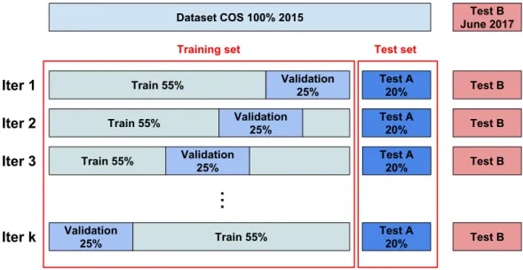
In a frame of a supervised classification scheme, traditionally, people split training data during the classification into two sets: Train and Test. Both correspond to a fixed random choose where the model is then iteratively trained using the train set (i.e 70%) and validated using the test set (i.e 30%). Alternatively, the are many ways to split the training dataset, and this arrange is usually called cross validation. Unlike the previous arrange, we can generate multiple splits of the train set, so that we only fixed the initial test set (i.e 30% TA). This fractions parts of the train set correspond to several splits (k-folds) of the train set (i.e 55% train and 25% validation). This allowed us to estimate unbiased parameters and generate stable predictions. In Figure 4.6 we can appreciate how we made this multiple splits during the classification.

We performed a pixel based classification using RF and SV classifiers. The classification models were built from each train set after carefully carrying out a

4 Methodology Training set Dataset COS 100% 2015 Train 55% Validation 25% Test A 20% Train 55% Validation 25% Train 55% Validation 25%

...

Figure 4.6: A visualization of the splits of the training dataset during classifica-tion

sensitive analysis of the parameters. In SVM, two condition were tuned; gamma in the insensitive-loss function and and the cost of constraints violation C , while the radial kernel function was left default. In RF, the number of variables ran-domly sampled as candidates at each split (mtry) and the number of trees to grow were tuned (ntree).

It should be noted, that we only had one independent dataset (TB) for only one image in June 2017. Therefore, the only image with a test using an updated dataset is June 2017, the rest of the images used a fraction part of the sampling of the out-up-date map to test the results.

4.5 Filtering training data

While the training data selection is automatic (see section3.3), this thesis aimed to refine the training data for each period of analysis in order to evaluate better accuracy in the classification. In this context, we used two different techniques, one based on trimming NDVI values per class depending on how far they are from their normal dispersion and another that consider an iterative learning procedure.

4.5 Filtering training data

4.5.1 Trimming NDVI signals

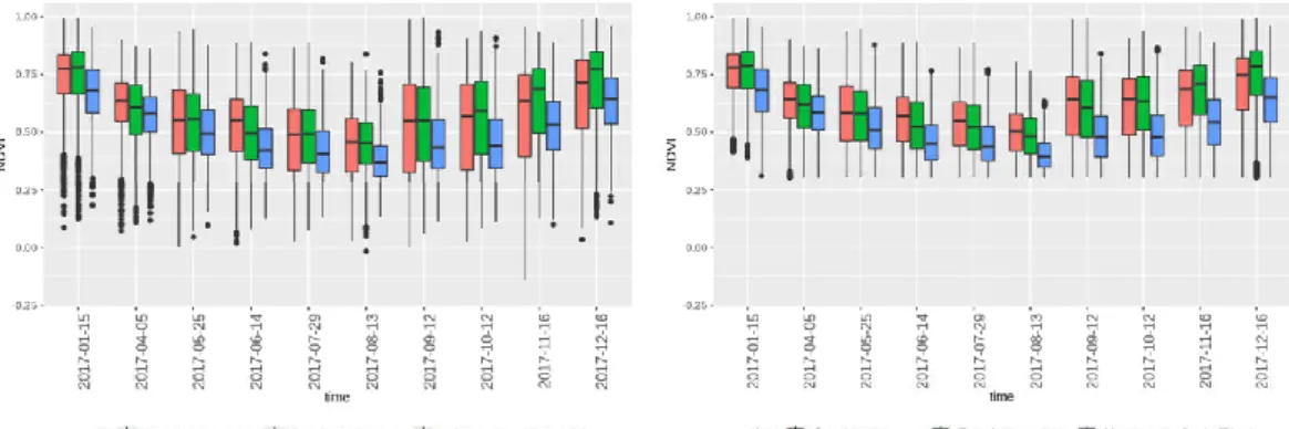
We recreated the NDVI values for all points through 2017 year. In this sense, we made box-plots in order to see the dispersion of NDVI values per class and time. Figure 4.7 shows one example of the variability of three woody classes over the year 2017. The box-plots display interquartile ranges (IQR, size of the box), maximum and minimum values (limits of the whiskers) and possible outliers (black points) per scene.

Figure 4.7: NDVI signals over time for classes of trees

Labels can intersect pixels with a mixture of classes and, therefore, display different spectral signatures to the usual ones. In the context of trees, depending on the canopy, the distances between trees plantation is diverse. Among the re-maining spaces of the trees, other types of vegetation can grow up, such as bushes or grass. Therefore the variation of NDVI may be a result of how saturated or dispersed is the biomass for the specific pixel. For example, the slight increase of the median of NDVI values for trees during the beginning and the end of the year correspond to an increase of a photosynthetic activity due to rainy periods. Therefore, the fractional proportion of the class tree in the pixel tends to satu-rate more the pixel with respect the other fraction that consider other types of vegetation. Generally, class trees should display NDVI values larger than 0.3, so that we decided to remove samples with NDVI values lower than this value. Moreover, samples with NDVI values beyond 1.5 times the IQR, from the first or third quartile were removed from the data. That is, black points located beyond

4 Methodology

the length of the whiskers (see Figure 4.7).

4.5.2 Filtering training data based on a iterative learning

procedure

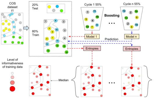
The second strategy for removing possible anomaly data hindering the results of the classification was based on iterative learning procedure. That is, before the learning step, all the train set (80%) is subject to a quality evaluation in order to define the level of contribution of each point in the classification.

Using multiple splits of the training dataset (55% train, 25% validation), we recreated multiple models in order to classify itself. After that, we evaluated the level of uncertainty in every prediction using the measurement of information entropy (see Equation 4.2).

S = n X

i

pilog(pi) (4.2)

If a point was informative for the classification, that is, a point correctly predicted over different splits, then the point depicted low entropies values. After that, we normalized and inverted the entropies values in order to define a score of informativeness per point (see figure 4.8).

As lower the score, the larger the chance of the point to be removed from the training for a specific iteration. Each iteration removed 2.5% of points from the train set, so that, we repeated the process of calculating informativeness and took out points up to the specific definition of points in the train set led to stop a possible increase in the overall accuracy and reduce the predictive power of the classifier.

4.6 Evaluation of the robustness of the classifiers

To asses the classification results, we proposed to add noise to the COS dataset. Independently of the inherent noise of the out-up-date data, we decided to inject in the train set different levels of noise to evaluate their impact in the overall accuracy.

4.6 Evaluation of the robustness of the classifiers

...

...

Figure 4.8: Iterative learning procedure to define informativeness based on boost-ing and the measurement of information entropy

The random and systematic injection of noise consist of selecting a set of points and change their original labels for one of the rest of the classes. Each injection covered 5% of the train. We performed classification using both RF and SVM considering a tune of parameters per injection.

5 Results

While this thesis aimed to make automatic the production of intra-annual maps implementing a workflow that consisted of supervised classification in synergy with automatic extraction of training samples from an old map, it also aimed to use singular and BAP composites. In this context after selecting the training data from COS 2015 automatically (Chapter 5.1), we defined a baseline to compare the classification results both using imagery that matches the year of production of the map, and imagery for the date of analysis 2017 (Chapter 5.2). After that, we set out the classification both the seasonal composites and the singular imagery; we performed an accuracy assessment based on the confusion matrix and OA (Chapter 5.3). The obtained results questioned if quality control over the training data can result in better accuracy (Chapter 5.4), and how robust are the classifiers in the presence of several levels of noise in the training data during the modeling (Chapter 5.5).

We implemented the methodology using scripts written in Python and R languages. Readers interested in the application of these procedures can visit the following link in GitHub .

5.1 Automatic training selection from COS map

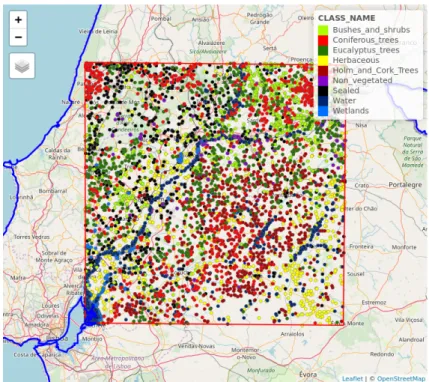
Figure5.1 shows the spatial distribution of the equalized random sampling done over the study area. For the first dataset composed of nine classes, we selected 1000 samples per class for the categories of Shrubs, Coniferous trees, Eucalyptus trees, Holm and cork trees, Herbaceous, no vegetated areas, sealed surface, water surfaces, and wetlands. Instead, the second dataset composed of six classes, it

5 Results

comprised 1000 samples per class samples for the categories of Woody, Herba-ceous, no vegetated areas, sealed surface, water surfaces, and wetlands.

Figure 5.1: Spatial distribution of the training data

In this context, after the atmospheric and radiometric correction of the im-agery, we extracted the spectral information per sample using imagery that came from 2015 and 2017.

5.2 Classification

Generally, classification accuracy depends on multiple factors, where the nature of the training samples, the number of features (bands and ancillary data), the number of classes to be discriminated, the spatial resolution of the images and the properties of the classifier are the most important. From this angle, we set out the evaluation of the accuracy of the classification influenced by the previous factors for one image in 2015 in order to use it as a baseline to judge the results over 2017.

5.2 Classification

5.2.1 Baseline

Figure5.2 shows a comparison of OA in the classifications of one image on July 25 of 2015 using two different number of classes and two different number of bands(features). On the one hand, from the number of bands, we evaluated the adding value in the OA after including ancillary data in addition to the spectral in-formation that came from Sentinel 2. The three additional features corresponded to NDVI, DEM, and Slope. The addition implied a significant increase in accu-racy for the discrimination of classes in both dataset of six and nine classes; 5.0 scores and 3.0 scores respectively. On the other hand, the predictive power of RF increased after merging shrubs and trees variability in only one class called Woody. Therefore, the implementation of updated reference data extracted from COS map in a supervised classification of one image in July 2015 using 13 bands resulted in accuracies of 0.61 and 0.73 for the datasets of six and nine classes respectively. 0.68 0.73 0.58 0.61 6 Classes 9 Classes 10 13 10 13 0.00 0.25 0.50 0.75 1.00 Number of Features Accurac y

Classes a 6 Classes a 9 Classes

Figure 5.2: Baseline July 25 2015, RF classifier

Even though machine learning algorithms can be considered methods based on a black-box supervised learning, they can also give an intuitive explanation about the predictive power of the features in the classification. According to the documentation of Sklearn (library Python), RF offers a score that measures the

5 Results

importance of the study variables based on the mechanism of out-of-bag-sample error. In figure5.3, we show scores of the variables after implementing RF (results were the same for all the imagery). As higher the score, higher the predictive power of the variable. Notably, in terms of spectral information, the bands NDVI, B11-SWIR, and B12-SWIR, showed the highest scores. This pattern may obey to the fact that the dataset was mainly composed of classes with vegetation. Moreover, the DEM also was a good predictor, determining that the elevation fractionally characterizes the land cover system in the region.

Figure 5.3: Level of importance variables random forest

5.2.2 Classification using RF and SVM (images 2017)

Figure5.4 shows a general evaluation of the classification of images in 2017 using as reference the training data selected from COS map 2015; classification per image considered a careful sensitive analysis of the parameters of the classifiers. In summary, the implementation of SVM with a RBF kernel outperformed the results obtained with RF over all the imagery of 2017 with average differences of 2 scores.

In practice, the selection of the images are conditioned for the level of cloud contamination, and therefore best images are selected from the time of the year less affected by cloud cover like those from Summer. According to the technical

5.3 Single maps vs seasonal maps 0.75 0.72 0.740.75 0.720.74 0.730.75 0.740.76 0.740.75 0.730.74 0.730.74 _0.70.72 _0.710.73 0.62 0.59 0.60.62 0.60.62 0.610.62 0.620.64 _0.60.63 0.610.62 0.610.63 0.60.61 0.60.62 6 Classes 9 Classes J an.15 _Apr .05 Ma y.25 J

un.14 Jul.29 _Aug.13

Sep .12 Oct.12 _No v.16 Dec.16 0.00 0.25 0.50 0.75 1.00 0.00 0.25 0.50 0.75 1.00 Singular Images 2017 Accurac y Model a RF a SVM

Figure 5.4: Perfomance classifiers RF and SVM, scene-based composites 2017

report of COS map, the Aereo-photographies were taken during April, May, and June of 2015. The match in season between image acquisition and the date of the images of reference for the production of COS map can be one of the reasons by which around these dates we had slight better results. Generally, the results ranged between the same range of accuracies than for 2015. We highlighted the OA of July 29 where the score was slightly higher respect to the rest of the images: 0.76 and 0.64, dataset with 6 and 9 classes respectively. This scenario showed first insight into the robustness of the classifiers in the presence of possible changes in the reflectance during the year due to phenology.

5.3 Single maps vs seasonal maps

We proposed two examples of intra-annual mapping, one using single images and other using seasonal composites. Regarding the construction of the composites, the computational performance of a methodology based on maximum NDVI for their construction was quite fast. Depending on the number of spectral bands and images per date to consider, the scripts developed on Python could create

5 Results

composites with Sentinel 2 imagery in terms of few minutes. Figure 5.5 shows one example of how the composites combated the cloud contamination of some images during the production of one composite in Spring. Clouds tend to depict red reflectance somehow larger than the near infrared. This slight difference turns out in low positive or negative values of NDVI. When the clouds passed over land covers such as vegetation, the maximization of NDVI was a simple mechanism that allows to retrieve the best pixels associated to high values of NDVI, and therefore, the construction of artificial images free of clouds.

The production of BAP composites raised the curiosity for comparison in the classification performance between single images and composites. In the case of classification of a dataset with six categories, Figure5.6 shows the classification evaluation using OA for the best singular images per season vs. the BAP com-posites. The results showed equivalent OA for all the images based in the same range of variation of the OA after cross-validation.

Moreover, with the same above specifications we compared the accuracies of the dataset with nine classes (see Figure 5.7 ). In summary, composites seem to give the same valuable information than pure single images for the discrimination of land cover classes. Unlike, single images, BAP composites per season are cloud-free and phenomenologically more consistent for the production of seasonal LULC mapping.

To describe the performance of the classification models per classes we cre-ated the normalized confusion matrix (see Figure5.8). Particularly, this matrix represented the predictive power of the classifier SVM with RBF kernel in the discrimination of nine classes using an image of July 29 of 2017. From this angle, the values of the diagonal elements represented the degree of correctly predicted classes. The confusion is expressed by the false classified off-diagonal elements, since they may be mistakenly confused with the rest of classes. We warn the read-ers for possible underestimation on accuracy since the validation of these results are based on a test set that also contains samples from an old map. Besides that, we calculated the kappa index and accuracies for omission and commission (see table 5.1). The accuracies in the diagonal of the confusion matrix corresponded

5.3 Single maps vs seasonal maps 8°54'0"W 8°57'0"W 39 °2 1' 0" N 39 °1 8' 0" N 8°54'0"W 8°54'0"W 8°57'0"W 8°57'0"W 39 °2 1' 0" N 39 °1 8' 0" N 8°54'0"W 8°54'0"W 8°57'0"W 8°57'0"W 39 °2 1' 0" N 39 °1 8' 0" N 8°54'0"W 8°57'0"W NDVI High : 1 Low : -1 8°54'0"W 8°57'0"W 39 °2 1' 0" N 39 °1 8' 0" N 8°54'0"W 8°57'0"W 8°54'0"W 8°57'0"W 39 °2 1' 0" N 39 °1 8' 0" N 8°54'0"W 8°57'0"W 39 °2 1' 0" N 39 °1 8' 0" N

April 5 April 15 May 25

SPRING COMPOSITE

Figure 5.5: pixel-based composite Spring

to the producer accuracy. The proximity of Cohen’s kappa and OA statistics explained a high agreement between the user and producer accuracy. That is, classification accuracies both for omission and commission have similar results.

Regarding the classification of the dataset with nine classes, We could di-vide the predictive power of the model in three categories. Firstly, classes that contained woody such as Shrubs and Trees are showing a low predictive power

5 Results 0.6 0.6 0.62 0.62 0.61 0.61 0.6 0.6 0.62 0.62 0.64 0.63 0.62 0.62 0.62 0.62

RF

SVM

Singular Image vs BPA

Accurac

y

Season a _Spring a _Summer a _Autumn a _Winter

Figure 5.6: Performance of the classifications, single images vs BPA composites, 9 classes classification 0.74 0.72 0.74 0.73 0.73 0.73 0.71 0.7 0.75 0.74 0.75 0.75 0.74 0.74 0.73 0.72

RF

SVM

Singular Image vs BPA

Accurac

y

Season a _Spring a _Summer a _Autumn a _Winter

Figure 5.7: Performance of the classifications, single images vs BPA composites, 6 classes classification

of the model to discriminate and identify them; with ranges between 0.48 and 0.58. Specifically, the confusion of these classes was concentrated among them; that is why a merge of these classes in Woody for the second dataset ended up in

5.3 Single maps vs seasonal maps

Figure 5.8: Normalized confusion matrix, classification scene-based composite July 29

an increase of the accuracies for all the classes (see table 5.2). Secondly, classes such as wetlands and water depicted high predictive power of the model to pre-dict them in comparison with the above classes; 0.85 and 0.92 respectively. The good perform for wetlands, and water surfaces could be a consequence of the proportion of the sampling respect to the size of the land cover classes. For ex-ample, Water and wetlands sum up an area that covered only 1.5% of the study area in comparison to 38% of classes with woody. Therefore, even though the classification was in balance keeping the same number of samples per class, the representativeness of the sampling in proportion is entirely different. Finally, the predictive power of the model to classify herbaceous, sealed and no vegetated corresponded to level medium. The model still weakly predicted these classes probably due to the presence of mixture classes in the pixels. Therefore, instead of pixel-based classification, future attempts can approach sub-pixel models.