Exploiting the bead injection LOV approach to carry out spectrophotometric
assays in wine: Application to the determination of iron
Susana S.M.P. Vidigal
a, Ildikó V. Tóth
b, António O.S.S. Rangel
a,∗aCBQF/Escola Superior de Biotecnologia, Universidade Católica Portuguesa, Rua Dr. António Bernardino de Almeida, 4200-072 Porto, Portugal bREQUIMTE, Departamento de Química, Faculdade de Farmácia, Universidade do Porto, Rua Aníbal Cunha 164, 4090-030 Porto, Portugal
Keywords:
Solid phase spectrometry Sequential injection lab-on-valve Bead injection
Iron Wine
A sequential injection lab-on-valve (SI-LOV) system was used to develop a new methodology for the determination of iron in wine samples exploiting the bead injection (BI) concept for solid phase extrac-tion and spectrophotometric measurement. Nitrilotriacetic Acid (NTA) Superflow resin was used to build the bead column of the flow through sensor. The iron (III) ions were retained by the bead column and react with SCN−producing an intense red colour. The change in absorbance was monitored
spectropho-tometrically on the optosensor at 480 nm. It was possible to achieve a linear range of 0.09–5.0 mg L−1
of iron, with low sample and reagent consumption; 500 mL of sample, 15 mmol of SCN−, and 9 mmol of
H2O2, per assay. The proposed method was successfully applied to the determination of iron in wine,
with no previous treatment other than dilution, and to other food samples.
1. Introduction
The chemical composition of wine is very variable and com-plex; besides the main organic compounds such as ethanol, sugars, organic acids, polyphenols and proteins, wine also contains sev-eral inorganic species dissolved[1–3]. Some trace metals can also affect the organoleptic characteristics of the wine, including the flavour, freshness, aroma, colour, and taste[1]. Moreover, the con-tent of some metals can be used to prove wine authenticity and quality. It is known that concentrations higher than 5 mg L−1can cause several changes on the stability of the product and can pro-mote oxidation and wine aging[4,5]. The natural concentration in wine depends principally on the type of the soil where the grapes are produced[2,6–8]. The official method recommended for the determination of iron in alcoholic beverages by OIV and AOAC is based on atomic absorption spectrometry (AAS), either with flame or with furnace atomisation, and is the most widely used method for this determination[3,9].
Molecular absorption spectrophotometry has been the most common detection method used to quantify chemical components [10], but not so common in wine analysis. This might be due to a number of reasons associated with the complexity of the wines. To begin with, metals can be present in wines in different forms, either free or bound to different ligands. Therefore, if the total con-tent is aimed, metals have to be released before or during the colour reaction, either by simple acidification for labile species or by
carry-∗ Corresponding author. Tel.: +351 225580064; fax: +351 225090351. E-mail address:[email protected](A.O.S.S. Rangel).
ing out drastic mineralisation procedures. There are also potential interferences in the colour reactions with a major difficulty aris-ing from the intrinsic colour of the wine. Different flow analysis approaches, like reversed flow[11], merging zones[12], multi-site detection[13], or use of in-line dialysis[14], have been proposed to tackle this problem. Even so, if the background absorption is very high, the first two approaches may not be efficient, while the use of in-line dialysis might induce a too high dilution. Additionally, in dialysis flow analysis systems, it is difficult to match the diffu-sion yield of standards and samples, which make difficult to obtain accurate calibration procedures.
Solid phase extraction (SPE) can be an attractive alternative to the above-mentioned processes, because it might provide the pre-concentration of the analyte and the discard of interfering agents. In the traditional SPE concept, the detection will occur on the eluted phase; however there is a partial loss of preconcentration capabil-ities gained in the sorption step[15]. To enhance sensitivity, solid phase spectrometry (SPS) has been developed based on the direct measurement of the light attenuation of adsorbent particles packed in an optical cell, in which the target analyte is concentrated and coloured[10]. Considering that the measurement occurs without elution, SPS turns to be a more sensitive method than the con-ventional SPE. SPS can be performed by two different approaches: batch or flow method. To employ the batch method, besides being very time-consuming, above-average skills are required to pack the solid particles into the cell. The flow methods are more suitable since they can easily measure the light attenuation in the adsorbed species in the flow-through cell with considerable reduction of the volumes used. However, the implementation of SPE/SPS in flow systems can be tricky, as the solid phase can become too much
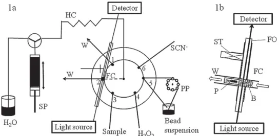
Fig. 1. (a) Configuration of the BI-LOV manifold. (b) Position of the bead column in the flow cell. SP, syringe pump; PP, peristaltic pump; HC, holding coil; FC, flow cell; SCN−,
1.5 M; H2O2, 0.3 M; W, waste; ST, PTFE stopper, P, PEEK plug; B, beads; FO, fibre optics.
packed and increase overpressure. Additionally, if it is not renewed, it might become saturated, either with the analyte or with the inter-fering compounds. To overcome this problem, instead of reusing the particles, it would be interesting to renew the optosensor. This is quite feasible using sequential injection, lab-on-valve approach (SI-LOV)[16,17]. The association of SIA with SPS leads us to the con-cept of bead injection (BI), based on the introduction and trapping of the functionalized beads in the flow conduit[18]. Beads are used as a solid surface to extract the analyte or to accommodate a chem-ical reaction. A precise volume of sample can be transfused through the bead surface allowing analyte separation and concentration. In the BI format, initially a small amount of micro-spheres is injected into the flow channel, where the beads are trapped and perfused by analyte solutions and auxiliary reagents. The reaction takes place on the bead surface allowing real time monitoring, directly on the solid phase, SPS, or on the eluted liquid phase, SPE[16]. When the bead column is placed in the detection zone it is labelled as flow-through sensor[19]. In some applications, after the measurement, the beads can be discharged, occurring physical regeneration, or in other cases the sensor surface can be renewed, being considered as chemical regeneration. The physical regeneration of the sensor is an advantage since there is no need for the elution step and its appli-cability is not limited by the lifetime of the sensor, at the same time any possible contamination is also eliminated. The major interest of using these sensors is the increase on sensitivity and selectivity. The sensitivity is augmented since the analyte is retained in the detection zone, and the selectivity also increases since interfering species are excluded from the bead column, therefore they do not develop any signal. In SPS assay, when the chemical reaction takes place on the bead surface, the baseline must be established after the application of the sample mixture to the bead column. In this way the interference of the colour of the sample can be also reduced. The main difficulty of this approach is to obtain a solid phase that can be applied to the separation, concentration and determination of the chemical species of interest[18].
Beads of different material nature are commercially avail-able and have become useful as surface media for retaining reagents, analytes or reaction products. Sephadex is usually used for the linkage of reagents; Sepharose 4B; agarose; and Aminolink, which provide adequate bead support for bioligand immobiliza-tion; Cytopore is the most usual for cell linkage [20]. For the determination of metallic ions several types of beads have been used; Sephadex[19]and Chelex-100[21]beads have been applied for total iron determinations. The present work employs a
com-mercial available “Nitrilotriacetic Acid (NTA) Superflow resin” which can isolate and concentrate dissolved iron at low pH[22]. This resin was originally designed for high throughput sam-ple clean-up procedures based on the affinity chromatography concept. Recently, NTA Superflow resin was applied for the pre-concentration of total iron in sea[22,23] and river[24] water samples.
The herein proposed methodology exploits the concept of solid phase spectrometry in a SI-LOV format to circumvent some dif-ficulties associated with complex matrices in spectrophotometric measurements, namely a high background sample absorption; it was applied to the determination of iron (III) in wines. At low pH (ca. 2) the Fe (III) ions are retained in the bead column and react with thiocyanate reagent. As a result of the reaction, an intense red colour is produced and is spectrophotometrically monitored at 480 nm.
2. Experimental
2.1. Reagents and solutions
All solutions were prepared from analytical grade reagents, and deionised water (conductivity < 0.1 mS cm−1) was used throughout the work.
The thiocyanate solution was prepared by dissolving 11.4 g of NH4SCN in 100 mL of water. The hydrogen peroxide solution (0.3 M) was prepared from the stock solution (Perhydrol, 30% H2O2). The iron (III) stock standard solutions (up to 5 mg L−1) were prepared by diluting commercial 1000 mg L−1iron atomic absorption standards (iron standard solution, iron (III) nitrate, VWR-Spectrosol) in 0.01 M HCl solution. The iron (II) stock standard solution (100 mg L−1) was prepared by dissolving (NH4)2Fe(SO4)2·6H2O in 0.01 M HCl solu-tion.
The bead suspension used was a dilution in water to half (w/w) of the commercial stock solution (NTA Superflow resin, highly cross-linked 6% agarose, 60–160 mm of bead diameter, 50% sus-pension in 30% ethanol, 30510, Qiagen).
2.2. Samples
The wine samples analysed (red table, white table and port wine) were purchased in a local market. When necessary, dilution was carried out as sample pre-treatment. The other samples, olive and soybean brines were purchased in a local market, and had no
other sample pre-treatment than filtration followed by dilution, when necessary.
2.3. Apparatus
The SI-LOV system (FIAlab-3500, FIAlab Instruments, Medina, WA, USA) presented inFig. 1, consisting of a bi-directional syringe pump (2500 mL of volume), a holding coil, a bi-directional variable speed peristaltic pump, and a lab-on-valve manifold mounted on the top of a six-port multi-position valve, was used. As detection system, a USB 2000 Ocean Optics, charge coupled device (CCD) spectrophotometer equipped with fibre optics (FIA-P200-SR; id: 200 mm), and a DH-2000-BAL Mikropack, UV/VIS/NIR light source, was used. FIAlab for windows 5.0 software on a personal computer was used for flow programming and data acquisition. The bead col-umn was built between the two optical fibres (Fig. 1b) and a plug (small piece of yellow PEEK tubing, # 1536, Upchurch Scientific). 2.4. Flow procedure
The SI-BI-LOV flow procedure is summarised inTable 1. The ini-tial steps of A–C, consisted in the preparation of the bead column in the flow cell, where 40 mL of the bead suspension was packed in the flow cell by 80 mL of carrier at 10 mL s−1. Afterwards, the sample and the oxidant were aspirated in a following sequence: 10 mL of H2O2; 250 mL of sample; 10 mL of H2O2; 250 mL of sample; 10 mL of H2O2. Then, the sample mixture perfused the bead column in the flow cell; afterwards the reference scan was performed to estab-lish the absorbance baseline. The change in the absorbance was monitored at 480 nm while 10 mL of SCN−drove through the bead column. After the measurement, the physical regeneration of the flow-through sensor was carried out by the aspiration of the beads to the holding coil and subsequent discharging to waste.
For cleaning the sample circuit, the analytical cycle was stopped and diluted acid-and-base solutions were sequentially passed through the flow cell, followed by water for rinsing. At the end of the washing cycle, the blank absorbance was registered and, if this value approached the original one, the system was assumed to be cleaned.
2.5. Reference method
A reference method was performed to corroborate the results obtained by the developed method. The method used was a Portuguese reference method [25]for the determination of iron content in alcoholic beverages and spirits by atomic absorption spectrophotometry.
3. Results and discussion 3.1. Study of the flow system
Several physical parameters like sample and reagent volumes, the aspiration sequence and the flow rates used in the flow system, were studied.
The repeatability of bead packing is an essential parameter to assure reproducible and good quality data. The first study was to select the strategy of how to introduce the bead suspension in the flow system. The option was made to keep the bead suspension circulating in a closed circuit connected to the port 5 (Fig. 1) of the LOV system. It is essential to maintain a well-stirred bead suspen-sion, since aspiration of beads from an unstirred sediment results in blockage of the bead aspiration channel. As the nature of the beads can tolerate magnetic stirring, this was the chosen procedure to maintain the beads suspended. A rotating container (placed in a Vortex shaker) was also tested and the repeatability showed no
significant difference when compared to the magnetic stirring. The NTA Superflow beads have a bead structure with relatively high percentage of agarose, this composition offers the beads low flow resistance, and easy handling possibilities inside the flow system. Still, the physical integrity of the beads had to be followed during the method development. The beads in agitation and circulation were kept under visual control, with the use of a microscope, and only after 4 days were possible to observe about 7% more of bro-ken beads when comparing with the freshly prepared suspension. Therefore the replacement of the bead suspension could be done weekly. Some physical parameters of the beads packing like: vol-ume of the beads suspension, carrier volvol-ume and flow rate were studied, since the light-path geometry must allow sufficient light to penetrate the bead layer and at the same time the target molecules must be on the optical path. The volume of bead suspension was studied in a range from 20 to 40 mL, while the carrier volume was studied in a range from 45 to 100 mL with a flow rate of bead packing of 2, 5 and 10 mL s−1. This study was carried out based on monitor-ing the increase of absorbance at 225 nm. The minimum volume of bead suspension used to construct the bead column was 25 mL; up to this volume of suspension there were no sufficient beads to make a reproducible sensor. The best loading conditions for the column preparation was selected based on the time required for establish-ing a reproducible bead column; it was set as 80 mL of carrier used to propel 40 mL of bead suspension at 10 mL s−1.
As this work is based on a solid phase reaction, the easiest way to establish the maximum binding capacity of the beads was to study the effect of the sample loading volume. The volume of sample was varied in a range from 100 to 600 mL. This study was performed with a 10 mg L−1Fe3+standard solution, 1.5 M of SCN−and 0.3 M of H2O2. Over 500 mL of sample, there was no significant increase on the analytical signal; therefore, 500 mL was the volume of sam-ple chosen for the work. In this case, the maximum load of Fe3+ corresponds to 250 mg Fe3+L−1of commercial beads suspension.
The flow rate used to propel the sample towards the bead col-umn was studied in a range from 3 to 15 mL s−1. The analytical signal increased with the increase of the flow rate up to 9 mL s−1. When the flow rate was augmented from 9 to 11 mL s−1, it was possible to observe an increase on the analytical signal of 10%, but at the same time the relative standard deviation of the signal increased from 2% to 5%, therefore as compromise between increase on the analytical signal and repeatability 9 mL s−1was chosen for further work.
With the physical conditions defined, the effect of the con-centration of the reagents on the analytical signal was studied. Calibration curves up to 8 mg L−1of Fe3+were performed. The con-centration of SCN−was set at 1.5 M and the volume of the reagent was altered to study its effect on the sensitivity of the method. When the quantity is augmented from 7.5 to 15 mmol per assay the sensitivity increased about 25%. Over this value, the linearity of the calibration curve is deteriorated; therefore the chosen quantity was 15 mmol per assay.
Given that the thiocyanate reacts with iron (III), it is necessary to ensure that the iron is in the oxidized form, thus an in-line oxidation is performed. Therefore, three steps were added to the analytical cycle, in order to sandwich the sample between oxidant (hydrogen peroxide) plugs. Since the plug of sample is long (500 mL) it was divided into two, and the oxidant was aspirated before, in the mid-dle, and after the sample. The volumes of oxidant were tested for 10 and 20 mL per plug. Different aspiration sequences were studied using a standard of 4.8 mg L−1Fe3+and 0.4 M hydrogen peroxide. It was possible to reduce the volume of the oxidant to 10 mL per plug since no significant loss on the analytical signal was observed. The concentration of oxidant was also studied in a range from 0.04 to 0.5 M and the analytical signal increased with the concentration of hydrogen peroxide up to 0.3 M. The analytical cycle was repeated with a 4.8 mg L−1of Fe2+solution and the results were similar to
Table 1
Flow protocol sequence of the developed method.
Step Description Volume (mL) Flow rate (mL s−1) Selection valve position
A Aspirate carrier to SP 1000 250 – B Aspirate beads to HC 40 20 5 C Propel beads to FC 80 10 2 D Aspirate H2O2to HC 10 50 4 E Aspirate sample to HC 250 50 3 F Aspirate H2O2to HC 10 50 4 G Aspirate sample to HC 250 50 3 H Aspirate H2O2to HC 10 50 4
I Send sample mixture to FC 1100 9 2
J Reference scan, absorbance scanning – – –
K Aspirate SCN−to HC 10 50 6
L Send SCN−to FC 75 3 2
M Aspirate beads from FC, by reversed flow 100 300 2
N Dispense beads to waste 425 300 1
those obtained with a standard of 4.8 mg L−1of Fe3+, therefore the 0.3 M concentration was chosen for further work.
The standard solutions of iron were prepared at pH 2. As wine samples have pH values around 3.5, the effect of the sample acidity on the reaction was also studied. Calibration curves were per-formed with standard solutions prepared in acidic medium at pH of 2 and at 3.5. The values obtained for the sensitivity of the curves at pH 2 and 3.5 showed no significant difference.
3.2. Study of interfering species
The study of potential interfering species was performed consid-ering the typical composition of wine samples. The effect of ethanol was studied in a range up to 20% (v/v) and there was no significant variation of the sensitivity of the method. Since wine has a com-plex matrix, the standards were prepared in a wine model solution containing 10% (v/v) of ethanol, 3 g L−1 of sugars (40:60; glu-cose:fructose), 7 g L−1of glycerol, 100 mg L−1of Mg2+, 100 mg L−1 of Ca2+, 50 mg L−1of Na+and 4 g L−1of tartaric acid, to evaluate the effect of matrix interference in the determination. There was no significant difference found on the sensitivity obtained in the anal-ysis of standards prepared in water and for the ones prepared in wine model solution, as it can be concluded from the values of the sensitivity obtained, 0.134 ± 0.008 and 0.137 ± 0.010, respectively.
3.3. Figures of merit of the method
The performance of the developed method was evaluated in terms of reagent and sample consumption, determination rate and dynamic range. The method presented a sample consumption of 500 mL per assay and a consumption of SCN−and H2O2of 15 mmol and 9 mmol per assay, respectively. It was possible to achieve a lin-ear range up to 5.0 mg L−1with a detection and quantification limits [26]of 0.02 and 0.09 mg L−1, respectively.
These figures of merit of the developed method are summarized inTable 2.
The operational stability of the developed system was calculated by performing the calibration procedure under identical physical and chemical conditions between different working days. A calibra-tion curve: Absorbance = 0.138 (±0.006) × [Fe3+] (mg L−1) − 0.004 (±0.024); the values in parentheses are the standard deviation for n = 8 calibration curves obtained from 5 standards injected 5 times each and performed in a period of five months. Stability can be con-sidered satisfactory, as this data reflects different batches of beads and reagents and daily preparation of standard solutions.
3.4. Sample analysis
A total of 12 (five white and seven red) table wines and four Port (two white and two tawny) wine samples were analysed. No other sample pre-treatment than dilution was required, for some of the samples. To evaluate the accuracy of the developed method, the reference method was also performed. The results obtained in the sample analysis are presented inTable 3.
The results obtained for the developed method are in good agreement with those obtained for the reference method. A lin-ear relationship: Cdeveloped meth.= mCcomp. meth.+ b, was established for the samples analysed, and the values obtained for the intercept (b) and for the slope (m) were −0.025 (±0.470) and 0.973 (±0.101), respectively. The values presented in parentheses are the limits of the 95% confidence intervals[26].
The previous table indicates that every red table wine sample had to be diluted. The main reason for this is not the high level of iron present but the natural colour of the matrix. Given that this is a spectrophotometric assay, the baseline absorbance must be established after the sample mixture contacts the bead column. For red table wines, this was not possible due to the natural colour of the matrix. The possibility to use a reduced sample volume as an alternative to the off-line dilution of the sample was tested. A red table wine with a volume of 150 mL, as opposed to 500 mL, was introduced in the system, packed between two plugs of 10 mL of H2O2. Even though a decrease on the sensitivity of the method of about 50% was observed, the result obtained for the analysis of a red table wine sample for the developed method (1.45 ± 0.19) was in good agreement with the result obtained for the reference method (1.4 ± 0.1). However, for other red table wine samples the same pro-tocol, did not allow to establish the baseline of the measurement. As a further reduction in the sample volume would decrease too much the sensitivity, we concluded that this approach could not be a general solution for every red wine.
Table 2
Figures of merit of the developed method.
Parameter Value
Reagent consumption per assay
SCN− 15 mmol
H2O2 9 mmol
Sample 500 mL
Waste production per assay 2.5 mL
Determination rate 20 det. h−1
Dynamic range 0.09–5.0 mg L−1
LOD 0.02 mg L−1
Table 3
Comparison of the results obtained for the analysis of wine samples by the reference and the developed procedures.
Sample Ref. met. (mg L−1)a SI-LOV (mg L−1)b RD%c Off-line treatment
White table wine 1 1.2 ± 0.1 1.4 ± 0.1 16.7 None
White table wine 2 2.1 ± 0.1 2.1 ± 0.1 0.0 None
White table wine 3 9.0 ± 0.4 9.2 ± 0.7 2.2 Dil. 4×
White table wine 4 6.1 ± 0.2 5.4 ± 0.1 −11.5 Dil. 4×
White table wine 5 2.2 ± 0.1 1.9 ± 0.2 −13.6 None
Red table wine 1 4.0 ± 0.2 4.1 ± 0.6 2.5 Dil. 4×
Red table wine 2 5.2 ± 0.4 5.0 ± 0.1 −3.8 Dil. 4×
Red table wine 3 5.5 ± 0.2 4.9 ± 0.6 −10.9 Dil. 4×
Red table wine 4 5.5 ± 0.4 5.4 ± 0.4 −1.8 Dil. 4×
Red table wine 5 5.4 ± 0.1 5.0 ± 0.1 −7.4 Dil. 4×
Red table wine 6 5.3 ± 0.4 6.0 ± 0.8 13.2 Dil. 4×
Red table wine 7 4.9 ± 0.2 4.3 ± 0.5 −12.2 Dil. 4×
Port, white 1 2.7 ± 0.2 2.6 ± 0.3 −3.7 None
Port, white 2 2.7 ± 0.4 2.6 ± 0.1 −3.7 None
Port, tawny 1 4.1 ± 0.4 3.9 ± 0.2 −4.9 Dil. 2×
Port, tawny 2 2.0 ± 0.2 2.1 ± 0.8 5.0 None
aMean and standard deviation for n = 3. bMean and standard deviation for n = 5. cRelative deviation.
As it can be concluded from Table 3, samples of red table wines and port wines presented distinct and typical concentra-tion levels, therefore other samples were also tested to assess the adaptability of the method to samples of non-wine origin and in different concentration ranges. A certified reference water sample and two different types of brines, olive and soybean, were analysed and the results obtained for the developed method were comparable to those obtained for the reference method (Table 4 in ESI).
4. Conclusions
The use of a lab-on-valve format with bead injection solid phase extraction proved to be a useful tool for the development of a molecular absorption spectrometry alternative to the atomic absorption spectrometry (AAS) reference method for the deter-mination of metals in complex matrices like wine. The proposed procedure also enabled to quantify the total content of the metal, with much simpler equipment. Based on the results (viz: good agreement with the reference atomic absorption procedure), it can be concluded that total iron is determined. This can be also deduced from the experimental conditions: the pH, the presence of an oxi-dant and a strong complexant and the additional off-line dilution of the samples contribute to the shift of the chemical equilibrium in a way that most of the iron originally present in a complexed form may be released, and made available in the form of Fe3+.
This flow system incorporating this optosensor also demon-strated to be a useful strategy to avoid interferences from complex matrices with high background absorption values, in a spectropho-tometric method. This was possible by using the bead injection procedure to separate the analyte from the matrix; taking advan-tage of the use of programmable flow. The chosen NTA resin proved to display characteristics appropriate for bead injection. The overall strategy could be adapted to other spectrophotometric determina-tions in complex matrices.
The results obtained for the analysis of several different food samples are in good agreement with the results obtained for the reference method. When comparing similar approaches[19,27,28] (Table 5 in ESI) the applicability of the developed SIA-BI approach was illustrated using various sample matrixes and in a highly auto-mated fashion.
Regarding the main limitations of the proposed method, we can point out the need for sample dilution if some red wines are anal-ysed. Another difficulty is the cleaning of the flow system after the analysis of red table wines; however, with additional port(s) on the
SI-LOV device, the cleaning protocol could be easily incorporated into the analytical cycle.
Acknowledgements
We gratefully acknowledge the support from the Laboratório de Química dos Servic¸os de Química e Organoléptica do CINATE, Escola Superior de Biotecnologia, Porto, Portugal. Susana Vidigal thanks Fundac¸ão para a Ciência e a Tecnologia (FCT) and FSE (III Quadro Comunitário) for the grant SFRH/BD/23040/2005. I.V. Tóth thanks FSE and MCTES (Ministério da Ciência, Tecnologia e Ensino Superior) for the financial support through the POPH-QREN pro-gram.
Appendix A. Supplementary data
Supplementary data associated with this article can be found, in the online version, atdoi:10.1016/j.talanta.2011.01.041.
References
[1] P. Pohl, Trends Anal. Chem. 26 (9) (2007) 941.
[2] S. Galani-Nikolakaki, N. Kallithrankas-Kontos, A.A. Katsanos, Sci. Total Environ. 285 (2002) 155.
[3] K. Pyrzy ´nska, Crit. Rev. Anal. Chem. 34 (2004) 69. [4] R.C.C. Costa, A.N. Araújo, Anal. Chim. Acta 438 (2001) 227. [5] C. Lasanta, I. Caro, L. Pérez, Chem. Eng. Sci. 60 (2005) 3477.
[6] M.A. Amerine, C.S. Ough, Methods for Analysis of Musts and Wines, Wiley, New York, 1974.
[7] M.G. Volpe, F. La Cara, F. Volpe, A. De Mattia, V. Serino, F. Petitto, C. Zavalloni, F. Limone, R. Pellecchia, P.P. De Prisco, M. Di Stasio, Food Chem. 117 (2009) 553. [8] R. Lara, S. Cerutt, J.A. Salonia, R.A. Olsina, L.D. Martinez, Food Chem. Toxicol. 43
(2005) 293.
[9] A. Santalad, R. Burakham, S. Srijaranai, K. Grudpan, Microchem. J. 86 (2007) 209.
[10] S. Matsuoka, K. Yoshimura, Anal. Chim. Acta 664 (2010) 1. [11] K.S. Johnson, R.L. Petty, Anal. Chem. 54 (1982) 1185.
[12] A.M.R. Ferreira, J.L.F.C. Lima, A.O.S.S. Rangel, Analysis 24 (1996) 343. [13] T.A.C. Oliveira, R.B.R. Mesquita, J.L.F.C. Lima, A.O.S.S. Rangel, J. AOAC Int. 88
(2005) 1511.
[14] A.O.S.S. Rangel, I.V. Tóth, Anal. Chim. Acta 416 (2000) 205. [15] M. Miró, W. Frenzel, Trends Anal. Chem. 23 (1) (2004) 11. [16] J. Ruzicka, Analyst 125 (2000) 1053.
[17] S.S.M.P. Vidigal, I.V. Tóth, A.O.S.S. Rangel, Talanta 77 (2008) 494. [18] R.P. Sartini, E.C. Vidotti, C.C. Oliveira, Anal. Sci. 19 (2003) 1653.
[19] M.J. Ruedas Rama, A. Ruiz Medina, A. Molina Díaz, Anal. Chim. Acta 482 (2003) 209.
[20] M.D. Luque de Castro, J. Ruiz-Jimémez, J.A. Pérez-Serradilla, Trends Anal. Chem. 27 (2008) 118.
[21] M. Miró, S.K. Kradtap, J. Jakmunee, K. Grudpan, E.H. Hansen, Trends Anal. Chem. 27 (2008) 749.
[22] M.C. Lohan, A.M. Aguilar-Islas, R.P. Franks, K.W. Bruland, Anal. Chim. Acta 530 (2005) 121.
[23] J. de Jong, V. Schoemann, D. Lannuzel, J.L. Tison, N. Matielli, Anal. Chim. Acta 623 (2008) 126.
[24] R.N.M.J. Páscoa, I.V. Tóth, A.O.S.S. Rangel, Microchem. J. 93 (2009) 153. [25] Norma Portuguesa, Alcoholic beverages and spirits, Determination of iron
con-tent by atomic absorption spectrophotometry, 1988, NP2280.
[26] J.C. Miller, J.N. Miller, Statistics for Analytical Chemistry, 3rd ed., Ellis Horwood, New York, 1993.
[27] P. Ampan, S. Lapanantnoppakhun, P. Sooksamiti, J. Jakmunee, S.K. Hartwell, S. Jayasvati, G.D. Christian, K. Grudpan, Talanta 58 (2002) 1327.
[28] K. Jitmanee, S.K. Hartwell, J. Jakmunee, S. Jayasvati, J. Ruzicka, K. Grudpan, Talanta 57 (2002) 187.