Behaviour of the contractual service margin on the general measurement model

M

ASTERS IN

A

CTUARIAL

S

CIENCE

M

ASTER

’

S

F

INAL

W

ORK

I

NTERNSHIP

R

EPORT

B

EHAVIOUR OF THE

C

ONTRACTUAL

S

ERVICE

M

ARGIN ON

THE

G

ENERAL

M

EASUREMENT

M

ODEL

M

ASTERS IN

A

CTUARIAL

S

CIENCE

M

ASTER

’

S

F

INAL

W

ORK

I

NTERNSHIP

R

EPORT

B

EHAVIOUR OF THE

C

ONTRACTUAL

S

ERVICE

M

ARGIN ON

THE

G

ENERAL

M

EASUREMENT

M

ODEL

E

STÊVÃO

M

IGUEL

C

ARDOSO

D

OMINGUES

S

UPERVISORS

:

C

ARLA

S

Á

P

EREIRA

H

UGO

B

ORGINHO

Abstract

IFRS 17 is the new international insurance norm that will start in 2022, bringing an unprecedented difficulty to the insurance world. From new quantitative requirements, to enormous computational engines. It is the new challenge for insurance companies and consultants throughout the world.

One of the new components of the norm is the Contractual Service Margin. This component reflects the unearned profit of a group of contracts. As insurance services are provided, this amount is released to the insurance revenue and it will affect the profit directly at each reporting period. We will test how it reacts when faced with unexpected events, different from the ones predicted at initial recognition.

Insurance companies will need to develop, or resort to, new calculation engines for the wave on information that is required for this norm. In this report, a fully automatic engine was built from scratch and, although it is calibrated for one specific type of contract, it has the potential to recognise all types of contracts. All results are merely illustrative, but demonstrate the importance of the Contractual Service Margin in this new norm.

Resumo

IFRS 17 é a nova norma internacional para seguros que irá ter início em 2022, provocando dificuldades sem precedentes no mundo segurador. Desde novos requisitos quantitativos, até motores computacionalmente avultados. É o novo desafio para as empresas seguradoras e consultores em todo o mundo.

Um dos novos componentes da norma é a Contractual Service Margin. Esta componente corresponde ao lucro não adquirido do grupo de contractos. Consoante os serviços prestados, este montante será lançado na insurance revenue e irá afectar directamente o lucro em cada período de reporte. Este é o tema principal do relatório e irá ser testado à força como reage face a eventos inesperados, diferentes daqueles que foram previsto no reconhecimento inicial.

Companhias de seguros irão necessitar de desenvolver, ou recorrer a, novos motores de cálculo para a onda de informação que será requerida pela norma. Neste relatório, um motor totalmente automático foi criado de raiz e, apesar de estar calibrado para um tipo de contracto em específico, tem o potencial de reconhecer todos os tipos de contractos. Todos os resultados servem para fins ilustrativos, mas demonstram a importância da

Contractual Service Margin nesta nova norma.

Acknowledgements

First of all, I would like to thank EY Portugal for granting me the internship opportunity. It was a great chance to start learning and gaining professional experience. As a consequence, I consider myself as a very lucky person to have had such an opportunity. I am also thankful for having met such a great team of professionals that led me through this internship. A special acknowledgement to Carla, Dora, Vanessa, Sílvia, Tiago, Inês, Maria, Daniela, and Ricardo.

I see this experience as a big milestone in my career, as it was the starting point. I will strive to use all skills and knowledge acquired during the internship in the best possible way, and will continue to work on them, in order to achieve my personal goals.

Second of all, I would like to thank ISEG for the experience and knowledge gained in the masters. Thank you to all the professors, for guiding me and my class in achieving our best possible results. More personally, I would like to thank my supervisor Hugo Borginho for all the advices and a constant helping hand when needed during the writing stage of this report.

Thirdly, I would like to thank all my friends that supported me during this time. To Elena, Francisco, Rogério and all others, thank you.

Next, I would like to give a special acknowledgement to my family, my mom, my brother, my sister and my cats, for being there for me when I needed and always giving moral support and care. And to my dad, thank you for always being there when help was needed, sometimes for more technical difficulties.

Lastly, I would like to give a special thanks to Carlota, for all the invaluable support and care throughout the last year and a half.

Index

Introduction ... 7

1 - International Financial Reporting Standards ... 8

2 - Level of Aggregation ... 9

3 - Fulfilment Cash Flows ... 10

4 - Interest Rate... 11

4.1 - Top-Down Approach... 11

4.2 - Bottom-Up Approach ... 11

5 - Risk Adjustment ... 12

6 - Contractual Service Margin ... 14

6.1 - CSM at Initial Recognition ... 14

6.2 - CSM at Subsequent Measurements ... 15

6.2.1 - Interest Accretion on the CSM amount ... 16

6.3 - Difference in Fulfilment Cash Flows Relating Future Service ... 16

6.4 - Amount of CSM recognized as P&L ... 17

7 - Coverage Units ... 18

7.1 - Quantity of Benefits ... 19

8 - CSM Calculation Engine ... 20

8.1 - Characteristics of the engine ... 20

8.1.1 - Contract Definition ... 20

8.1.2 - Cash Flows Core ... 20

8.1.3 - Coverage Units Core ... 21

8.1.4 - “ChangeTracker” ... 21 8.1.5 - Reporting Tables ... 21 8.2 - Contract Used ... 21 8.2.1 - Contract Conditions: ... 21 8.2.2 - Savings Account: ... 21 8.2.3 - Sample Characteristics: ... 21 8.2.4 - IFRS 17 Assumptions: ... 22 8.3 - Initial Recognition ... 22 8.4 - Subsequent Measurement ... 23

Introduction

This report will talk about the new buzz word in the insurance world, for the upcoming years, IFRS 17. It will be focus in one specific component of this norm, but giving some require overview of other fundamental topics of the norm.

It has a secondary goal, the construction of an engine to perform all calculation behind the final results. That is, all this will be as automatic as possible. With this engine, the student was able to use actuarial calculations learned in the masters and study the new norm.

This is the final work of ISEG’s master degree in Actuarial Science, with the support of EY Portugal, since they provided the opportunity for this internship. The internship took place between February and August of 2019. Not only was the student focused on the final work, but also had some experience with actuarial validations in the context of Solvency II, for the Solvency and Financial Condition Report, and conducting survey procedures for one insurance company in Portugal.

1 - International Financial Reporting Standards

The International Financial Reporting Standard 17 (IFRS 17) is the first specific and complete international accounting standard for insurance contracts. It needs to be applied by, not only insurance companies, but any entity that issues insurance contracts. In the case of Europe, only insurance companies can issue insurance contracts, so this topic is negligible in this case. It will replace IFRS 4 and be connected to IFRS 9, IFRS 13, and IFRS 15 (since these standards will help in several definitions and relations for, but not only, contracts with some financial instruments and measurements).

Fundamentally, IFRS 17 states that an entity shall identify insurance contracts that have significant risk, separate specified embedded derivatives from such contracts, divide them into homogeneous groups, and report base on that aggregation.

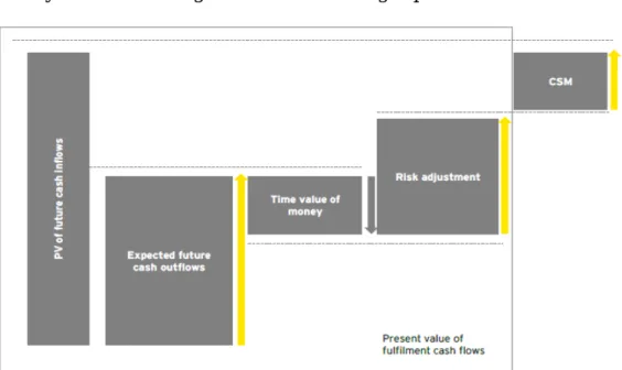
To be able to measure and apply it, entities will either use the General Measurement Model (GMM) or, if eligible, one of its two variations, Variable Fee Approach (VFA) or Premium Allocation Approach (PAA). Usually, entities will use the VFA when contracts are issued with profit sharing or some financial instrument within the contract. The PAA will be mostly used, because of its own design, on Non-Life insurance contracts, since one of its main characteristics is to have 1-year term contracts, although exceptions exist. After the contracts have been correctly separated by type, risk profile, cohort, and other characteristics, and the measurement model have been assessed, the entity shall determine the carrying amount for: the Liability for Remaining Coverage (LRC), which is comprised of the sum of the Fulfilment Cash Flows (FCF) and the Contractual Service Margin (CSM), and; the Liability for Incurred Claims (LIC). This two core components are in reference to the GMM. The PAA and VFA have variations of them, to address for each approach specificities.

The first component of the LRC, the Fulfilment Cash Flows (FCF), is comprised of an unbiased and probability-weighted estimate of future cash flows, a discount adjustment to present value to reflect the time value of money and financial risks and a risk adjustment for non-financial risk, as defined in Applying IFRS 17: A closer look at the

new Insurance Contracts Standard, from EY.

As for the second component of the LRC, the Contractual Service Margin (CSM), it represents the unearned profit that an entity will recognize as it provides service under the insurance contracts in the group, as defined in Applying IFRS 17: A closer look at the

2 - Level of Aggregation

At a conceptual level, the level of aggregation determines the unit of account to be used when applying IFRS 17 and affects the CSM and the level at which onerous contracts are identified and how the performance of the entity will be reported in its financial statements. One practice to be considered when determining this level is the pooling of similar risks using risk sharing. In summary, risk sharing is when insurance contracts in one group include conditions that can affect the cash flows of policyholders in a different group.

Using this very simplified example from the European Financial Reporting Advisory Group (EFRAG)’s paper on level of aggregation:

• Policyholder A has a contract with a minimum guarantee of 7% return and policyholder B has a contract with a minimum guarantee of 2% return.

• Both had an actual return of 5% in the current period.

• In this scenario, A will receive 7%, as stated on the contract, and B will only receive 3%, instead of 5%. This is because the extra 2% compensate for the 2% loss on policyholder A’s contract.

With this technique, the entity can prevent losses on individual contracts by using gains from the other individual contracts.

The concept of level of aggregation brings some issues when it comes to requirements in IFRS 17, such as (but not only): Applying the annual cohorts would require significant change to the entity’s systems and increase costs; The splitting of risk sharing amounts can be considered artificial and different from the current practices.

Another important aspect to mention is the requirements for the level of aggregation. The “Group Level” requirement. Essentially, IFRS 17 requires an entity to divide portfolios into a minimum of three groups:

• Contracts that are onerous at initial recognition, if any,

• Contracts that at initial recognition have no significant possibility of becoming onerous subsequently, if any,

• Remaining contracts in the portfolio, if any.

Onerous contracts are contracts that produce loss to the insurance company.

There is still discussion about what is “significant possibility” in this context, but it will be considered that none of the contracts will be, or will turn, onerous in this report.

3

- Fulfilment Cash Flows

Since this report is about the CSM, the PAA will not be addressed, as it is a simplification of the GMM and majority used on non-life insurers, as explained previously.

Both GMM and VFA have the same baseline measurement, but this report will focus on the GMM, and within, more specifically, the LRC. Within the FCF, the first element is to estimate the cash flows related to future service, i.e. future cash flows should, as defined in Applying IFRS 17: A closer look at the new Insurance Contracts Standard:

• Be within the contracts boundary; • Incorporate all information available; • Reflect the perspective of the entity; • Be current and explicit.

In the norm, there is a long list of examples of what can and cannot be considered as a cash flow within the contract boundaries, as well as what constitutes market and non-market variables and what it means to have explicit cash flows.

The second element is the discount rate and it must, as defined in Applying IFRS 17: A

closer look at the new Insurance Contracts Standard:

• Reflect the time value of money;

• Characteristics of the cash flows and liquidity characteristics of the insurance contracts;

• Be consistent with observable current market prices;

• Exclude effects of factors that influence such observable market prices, but do not affect the future cash flows.

According to IFRS 17, entities are intended to considerer a yield curve on the current market and adapt it to the characteristics of its own portfolio, by either choosing a risk-free rate like EIOPA and add an “Illiquidity Premium” or by choosing a yield curve that has similar returns to the entity’s assets and remove from it the risks that are non-existent in their portfolio.

The third and last component of the fulfilment cash flows is the Risk Adjustment (RA) for non-financial risks. The RA is stated to be the compensation that the entity requires for bearing the uncertainty about the amount and timing of cash flows that arise from non-financial risk, as defined in Applying IFRS 17: A closer look at the new Insurance

4 - Interest Rate

This is not the main topic of this report, so a very broad approach was done to be minimally coherent with this requirement.

As defined in the norm, an entity must use a yield rate term structure that best fits their contracts, i.e. it must reflect the time value of money, while taking into consideration all the characteristics of the cash flows and the liquidity of the insurance contracts, and be consistent with market prices, by taking the durations, liquidities and currencies of the contracts into account.

To do such fit, entities must choose between two possible approaches: • Top-Down Approach;

• Bottom-Up Approach.

4.1 - Top-Down Approach

The entity starts with an asset yield curve on the current market, based on assets like the ones that exist within the company, and takes the differences regarding amounts, timings and uncertainty of the cash flows between the assets and the insurance contracts. After that, it still requires taking out the market risk premium for credit risk.

4.2 - Bottom-Up Approach

The entity starts with a risk-free rate of a liquid bond, for example the EIOPA risk-free rate, and adjusts it to be an illiquid risk-free rate, using the illiquidity premium, as referred above.

Both approaches should deliver very similar yield curves, with immaterial difference between them, so it is a free choice to the entity.

In terms of anticipated difficulties on these two approaches, the Top-Down Approach will be less complex, due to the lack of definition of the term “illiquidity premium”. This method is currently in development and no concrete methodology is described in the norm.

For this report, it is assumed that the Bottom-Up Approach is chosen and the volatility adjustment of EIOPA will be considered as proxy for the illiquidity premium, for simplicity’s sake.

5 - Risk Adjustment

Again, since this is not the main topic of this report, a very broad approach was done here as well.

As stated before, the risk adjustment is expected to reflect the compensation an entity requires for bearing non-financial risk. It needs to be explicit and make the entity indifferent between fulfilling a liability that has a range of possible outcomes and a liability that will generate fixed cash flows with the same expected present value.

Although the IFRS 17 does not specify any technique to calculate the risk adjustment, there are some approaches that can be considered for that effect, mainly the Value at Risk (VaR), the Cost of Capital (CoC) and the Conditional Tail Expectation (CTE).

In this report, the RA technique will be based on the presentation given by Thomas Vehar and Hamdi Kacem, from the 3rd European Congress of Actuaries that happen is Lisbon 2019. It is based on the CoC approach. First, the entity needs to calibrate the central best estimate law (BE) for each risk factor and then calculate the deviation to a given level of confidence.

This deviation is calculated in the following way:

𝐷𝐷𝐷𝐷𝐷𝐷𝐷𝐷𝐷𝐷𝐷𝐷𝐷𝐷𝐷𝐷𝐷𝐷𝑡𝑡𝛼𝛼 = 𝐵𝐵𝐵𝐵𝑡𝑡𝛼𝛼− 𝐵𝐵𝐵𝐵𝑡𝑡 (1)

Where:

• 𝛼𝛼: 𝐿𝐿𝐷𝐷𝐷𝐷𝐷𝐷𝐿𝐿 𝐷𝐷𝑜𝑜 𝑐𝑐𝐷𝐷𝐷𝐷𝑜𝑜𝐷𝐷𝑐𝑐𝐷𝐷𝐷𝐷𝑐𝑐𝐷𝐷 𝐷𝐷𝑎𝑎𝑎𝑎𝑎𝑎𝑎𝑎𝐷𝐷𝑐𝑐; • 𝐷𝐷: 𝑅𝑅𝐷𝐷𝑅𝑅𝐷𝐷𝑅𝑅𝐷𝐷𝐷𝐷𝐷𝐷𝑅𝑅 𝑅𝑅𝐷𝐷𝑅𝑅𝐷𝐷𝐷𝐷𝑐𝑐

• 𝐵𝐵𝐵𝐵𝑡𝑡𝛼𝛼: 𝐵𝐵𝐷𝐷𝑎𝑎𝐷𝐷 𝐷𝐷𝑎𝑎𝐷𝐷𝐷𝐷𝑎𝑎𝐷𝐷𝐷𝐷𝐷𝐷 𝑤𝑤𝐷𝐷𝐷𝐷ℎ 𝐷𝐷ℎ𝐷𝐷 𝑅𝑅𝐷𝐷𝑎𝑎𝑟𝑟 𝑜𝑜𝐷𝐷𝑐𝑐𝐷𝐷𝐷𝐷𝑅𝑅 𝑎𝑎𝐷𝐷𝑐𝑐𝐷𝐷𝑅𝑅 𝐷𝐷ℎ𝐷𝐷 𝑐𝑐𝐷𝐷𝐷𝐷𝑜𝑜𝐷𝐷𝑐𝑐𝐷𝐷𝐷𝐷𝑐𝑐𝐷𝐷 𝐿𝐿𝐷𝐷𝐷𝐷𝐷𝐷𝐿𝐿 𝛼𝛼. The RA is then given by:

𝑅𝑅𝑅𝑅

𝛼𝛼

= 𝐶𝐶𝐷𝐷𝐶𝐶 ∗ �

𝐷𝐷𝐷𝐷𝐷𝐷𝐷𝐷𝐷𝐷𝐷𝐷𝐷𝐷𝐷𝐷𝐷𝐷𝐷𝐷 𝛼𝛼

(1 + 𝐷𝐷

𝑡𝑡+1

)

𝑡𝑡+1 𝑡𝑡≥0 (2) Where: • 𝐶𝐶𝐷𝐷𝐶𝐶: 𝐶𝐶𝐷𝐷𝑎𝑎𝐷𝐷 𝐷𝐷𝑜𝑜 𝑐𝑐𝐷𝐷𝑅𝑅𝐷𝐷𝐷𝐷𝐷𝐷𝐿𝐿; • 𝐷𝐷𝑡𝑡: 𝐼𝐼𝐷𝐷𝐷𝐷𝐷𝐷𝑅𝑅𝐷𝐷𝑎𝑎𝐷𝐷 𝑅𝑅𝐷𝐷𝐷𝐷𝐷𝐷 𝑜𝑜𝑅𝑅𝐷𝐷𝑎𝑎 𝐷𝐷𝐷𝐷 𝐷𝐷𝑅𝑅𝑅𝑅𝑅𝑅𝐷𝐷𝑅𝑅𝑅𝑅𝐷𝐷𝐷𝐷𝐷𝐷𝐷𝐷 𝑦𝑦𝐷𝐷𝐷𝐷𝐿𝐿𝑐𝑐 𝑐𝑐𝑎𝑎𝑅𝑅𝐷𝐷𝐷𝐷 𝐷𝐷𝐷𝐷 𝑦𝑦𝐷𝐷𝐷𝐷𝑅𝑅 𝐷𝐷;

This approach can be improved upon if entities gather, for at least 10 years, information about the risks their contracts are exposed to, study the changes and try to develop their

This goal might be the long term plan for entities, but at this moment it’s very complicated to estimate the risk distributions due to lack of information, since the probability of companies having kept track of this kind of data, for this amount of time, is very slim. But it might be a good topic to study and develop in the future, with the possible goal of comparing if the values of correlation between risks of Solvency II are or are not a good fit to reality, in terms of IFRS 17. And if not, trying to develop a technique to find what are the best values of correlation between risks for specific groups of contracts under IFRS 17.

6 - Contractual Service Margin

As stated earlier, the CSM is the unearned profit that the entity will recognize during the coverage period of the contract. This amount will not be recognized initially on Profit & Loss (P&L) but will be released steadily during the contract lifetime, to have the expected profits well distributed and not solely as a big profit recognized on day zero. This concept has two elements, the CSM at initial recognition, the moment when the entity recognizes the contracts, and the CSM at subsequent measurements, that is, each point in time that the entity confronts the predicted cash flows with real cash flows.

6.1 - CSM at Initial Recognition

By the definition present in the IFRS 17 standard, the amount of CSM will be equal to the negative of the sum of:

• The fulfilment cash flows;

• De-recognition of any asset or liability recognized for insurance acquisition cash flows and;

• Any cash flows arising from contracts in the group at the date.

This measurement will be exclusive to the recognition date and will be the key factor to determine if a contract is onerous or not. If, per chance, the CSM amount would be negative, i.e. net outflow, then the contract is no longer profitable and becomes onerous. The amount that would be recognised as CSM, since it is negative, it is recognised as

6.2 - CSM at Subsequent Measurements

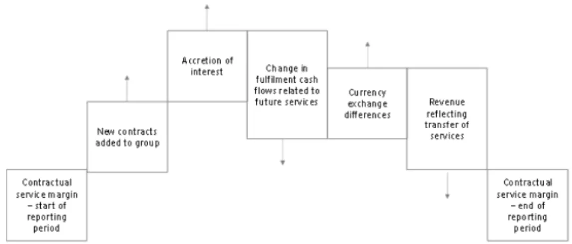
After the initial recognition date, the entity must measure the CSM in every reporting period, to evaluate the development of the profit. That is, to evaluate if the first day expectations are going as planned or if reality does not match alongside the predictions. To do such measurement, the entity must follow the definition present in the standard: update the fulfilment cash flows using current assumption and update the CSM to reflect changes provided in that period.

The CSM amount at the reporting period is equal to: • CSM amount at the previous reporting date • + Effect of new contracts

• + Interest accrued

• ± Difference in fulfilment cash flows relating future service • ± Effects of currency exchange differences on the CSM • - Amount of CSM recognized as P&L

This procedure is performed until the coverage period of the contract ends. The CSM can be applied at contract level, group of contracts level or cohort level. All have different positive aspects but also have negative setbacks as well, such as, but not only:

• For contract level, the CSM would reflect with much great detail each contract contribution to the entity. But it would demand a computational capacity that no entity would be willing to pay;

• For cohort level, the CSM would reflect the contracts as a whole, and even out the weight of onerous contracts. But it would need to develop a method for granulation of results. That is, it would need to show the auditors which amount of the CSM would be allocated to which group of contracts and why;

• For the group of contracts level, it would be the middle ground of the other two

In this report, it is assumed that the group of contracts is closed (which mean that there will be no new contract effects added) and that all currencies are the same, EURO (which makes the effect of currency exchange differences on the CSM null).

6.2.1 - Interest Accretion on the CSM amount

During the lifetime of contracts, interests will be accredited on the carrying amount of the CSM at each reporting period using the discount rate applied on initial recognition. So the entity must keep track of the assumptions at day zero. As discussed previously, the entity must obtain the yield curve best suited for the contract, cohort and/or portfolio, and it will be applied in this section.

One question that might be important to look upon is if the company should have a specific yield curve for each individual line of business, every individual cohort, or for all the portfolio. It may not be material the impact of different approaches in terms of the behaviour of the CSM, but it could be costlier to the entity, in terms of information storage and computational processes. IFRS 17 only provides guidance in this matter and no specific approach is said as preferable over another.

6.3 - Difference in Fulfilment Cash Flows Relating Future

Service

At each reporting date, the entity must re-evaluate the fulfilment cash flows. That is, the cash flows relating future service, the current discount rate and the current risk adjustment, except to the extent that:

• Increases in the fulfilment cash flows exceed the carrying amount of the CSM, and then resulting in loss or;

• Decreases in fulfilment cash flows are allocated to a loss component of the liability.

In other words, the entity must re-evaluate the fulfilment cash flows at each reporting period and, if the difference in FCF relating future service surpasses the carrying amount of the CSM at that time, then the CSM must not became less than zero and the remaining amount of the FCF is allocated to a loss component of the liability.

After that, it must calculate the difference of both amounts, the re-evaluated and the one at the previous reporting period. Again, huge potential for computational load for the entity. This difference is comprised into:

• Experience adjustment, arising from the premiums received in that period1_; • Changes in the expected present value of the future cash flows (EPVFCF) in the

• Expected Investment Component – Actual Investment Component. That is, difference between any investment component expected to become payable and the actual investment component that becomes payable in that period1;

• Changes in the risk adjustment for non-financial risks.

This experience adjustment is the difference between the premium receipts and the Insurance Service Expenses (except Insurance Acquisition Expenses). Insurance Service Expenses are the losses on groups of onerous contracts, and the reversal of such losses. In this report, it’s assumed that the experience loss will be zero at each reporting period, that is, all expected cash flows turn out to be the same exact value, at each reporting period. This represents a very simplistic approach to the CSM, and not at all realistic.

6.4 - Amount of CSM recognized as P&L

The last part of the CSM subsequent measurement is the allocation to the P&L, which is determine by:

• Identifying the coverage units in a group,

• Allocating the CSM equally to the coverage units for the current and future period and,

• Recognizing in P&L the final amount allocated.

The coverage units are the key component for the CSM and serve as the base for all CSM allocation in contract coverage period.

7 - Coverage Units

As defined in IFRS 17, and stated at the Transition Resource Group (TRG) meeting from February 2018, the coverage units establish the amount of the CSM to be recognized in P&L for services provided in a period, and the lowest form of coverage units allowed is the contract itself. A basic visualization of this concept can be grasped in the following example:

If company A has a group of contracts (G1) that recognized an initial CSM of 500 €, and it has a duration of 10 years, the amount of CSM allocated each period will be of 50 €, since the total amount of coverage units is 10, i.e. 1 coverage unit per year.

𝐶𝐶𝐶𝐶𝐶𝐶 𝑅𝑅𝐿𝐿𝐷𝐷𝑐𝑐𝐷𝐷𝐷𝐷𝐷𝐷𝑐𝑐 =_{𝑅𝑅𝐷𝐷𝑎𝑎𝐷𝐷𝐷𝐷𝐷𝐷𝐷𝐷𝑅𝑅 𝐶𝐶𝐷𝐷𝐷𝐷𝐷𝐷𝑅𝑅𝐷𝐷𝑅𝑅𝐷𝐷 𝑈𝑈𝐷𝐷𝐷𝐷𝐷𝐷𝑎𝑎 =}𝑇𝑇𝐷𝐷𝐷𝐷𝐷𝐷𝐿𝐿 𝐶𝐶𝐶𝐶𝐶𝐶 500 €_{10 = 50} (3)

Here is another example, but now considering the existence of different cohorts:

Take the same company A. Consider they have a second group of contracts (G2) with an initial CSM of 200 €, starting in year 2 (and first reporting year being year 3), and having a duration of 5 years. Using the same ratio as above, the company gets the following table:

Just for clarification, in G2, on the second reporting period, year 4, this is what the ratio above looks like:

𝐶𝐶𝐶𝐶𝐶𝐶 𝑅𝑅𝐿𝐿𝐷𝐷𝑐𝑐𝐷𝐷𝐷𝐷𝐷𝐷𝑐𝑐 =_{𝑅𝑅𝐷𝐷𝑎𝑎𝐷𝐷𝐷𝐷𝐷𝐷𝐷𝐷𝑅𝑅 𝐶𝐶𝐷𝐷𝐷𝐷𝐷𝐷𝑅𝑅𝐷𝐷𝑅𝑅𝐷𝐷 𝑈𝑈𝐷𝐷𝐷𝐷𝐷𝐷𝑎𝑎 =}𝑅𝑅𝐷𝐷𝑎𝑎𝐷𝐷𝐷𝐷𝐷𝐷𝐷𝐷𝑅𝑅 𝐶𝐶𝐶𝐶𝐶𝐶 120 €_{3 = 40 €} (4)

The goal of the coverage units is to distribute as evenly as possible how the CSM is recognized, not only at group level, but at cohort level.

Table 1 - Example of a CSM allocation with two groups of contracts

Years 1 2 3 4 5 6 7 8 9 10

G1 50 € 50 € 50 € 50 € 50 € 50 € 50 € 50 € 50 € 50 € G2 0 € 0 € 40 € 40 € 40 € 40 € 40 € 0 € 0 € 0 € Total 50 € 50 € 90 € 90 € 90 € 90 € 90 € 50 € 50 € 50 €

and should reflect the variability across periods in the level of coverage provided by the contracts.

The IFRS 17 standard defines it as:

𝐶𝐶𝐷𝐷𝐷𝐷𝐷𝐷𝑅𝑅𝐷𝐷𝑅𝑅𝐷𝐷 𝑈𝑈𝐷𝐷𝐷𝐷𝐷𝐷𝑎𝑎 = 𝑄𝑄𝐵𝐵 ∗ 𝐵𝐵𝐸𝐸𝑅𝑅𝐷𝐷𝑐𝑐𝐷𝐷𝐷𝐷𝑐𝑐 𝐷𝐷𝑎𝑎𝑅𝑅𝐷𝐷𝐷𝐷𝐷𝐷𝐷𝐷𝐷𝐷 𝐷𝐷𝑜𝑜 𝐷𝐷ℎ𝐷𝐷 𝐶𝐶𝐷𝐷𝐷𝐷𝐷𝐷𝑅𝑅𝐷𝐷𝑐𝑐𝐷𝐷 (5)

7.1 - Quantity of Benefits

For some time, the quantity of benefits did not have an explicit way to calculate, or even an explicit definition of what it might be. But in the TRG meeting in May 2018, it was agreed that there are three possible methodologies and the one that this report is based upon is the following:

• If the determination of coverage units reflects different levels of cover across periods, then it should be the level of cover provided in the current period and expected to be provided in the future ones;

• If it does not reflect different levels, then it should be based on the average benefits over the duration of the contract.

The methodology used further ahead to calculate quantity of benefits will be the expected value of such benefits, that is, it will considerer the second point above.

8 - CSM Calculation Engine

The second goal of this report was the construction, from scratch, of a CSM calculation engine. The idea behind it was, not only improving the student coding ability (in Visual Basic for Applications), but also to provide the company some starting point for the upcoming IFRS 17 engines required to help its clients.

Do to the unseen complexity and time restriction of the project, the goal changed from a full user-interactive CSM engine to a more simplified motor that only calculates the CSM behaviour for one type of contract: Endowment Contracts.

8.1 - Characteristics of the engine

The engine is comprised into 5 key components: • Contract Definition;

• Cash Flows Core; • Coverage Units Core; • “ChangeTracker”; • Reporting Tables.

8.1.1 - Contract Definition

All the main information about the contract and the reality at initial recognition, and the most current yield curve are store here, i.e. all the contract definitions, the yield curve that the entity chooses to use, the mortality table that will be applied, and more.

8.1.2 - Cash Flows Core

The base values of the cash flows are updated and exposed to the reality of mortality and lapses. There are also two more sheets on this core: the Cash Flows First Change and

Cash Flows Second Change.

In the sheet Cash Flows First Change, the engine saves the point in time where the first unexpected event happens and re-calculate all cash flows according to the new reality. In this case, since mortality is the only variable factor, it adjusts the exposer of each cash flow according to the new mortality rates.

In the sheet Cash Flows Second Change, the engine repeats the same logic, but starting from the point in time where the second unexpected event happen. All unexpected events are determined by the user.

8.1.3 - Coverage Units Core

The coverage units are calculated using the technique explain before. There is a sheet for initial recognition and for each unexpected event. Just as the cash flows, the three scenarios are collected in one unique table that will serve as base for the report table of the CSM.

8.1.4 - “ChangeTracker”

This specific component seeks and records the points in time where the reality differs from what was expected. For simplicity sake, it can record up to two changes from reality as the same run.

8.1.5 - Reporting Tables

For this project, only two tables will be presented: • The Initial Recognition Reporting Table and, • The Final Reporting Table.

8.2 - Contract Used

All cash flows were calculated from scratch based on a contract made by the student, and Endowment contract, with the following conditions:

8.2.1 - Contract Conditions:

o Premium of 3,678 € paid in the beginning of each year; o Maturity of 10 years;

o Death benefit of 35,000 € paid at the end of year of the policyholder death; o Survival benefit of 35,000 € + Savings account value paid at the end of the contract

life if the policyholder survives;

o Lapse benefit of 90% of the Savings account value paid at the end of the year that the policyholder lapsed;

o It’s assumed a lapse rate of 2% every year;

o Management expenses of 294 € paid at the end of each year; o Commissions in the value of 37 € paid at the end of each year.

8.2.2 - Savings Account:

o When the premium is paid, 2.5% of the premium goes to the savings account immediately;

o An annual 2% interest rate is applied to the account.

8.2.4 - IFRS 17 Assumptions:

o The coverage units will consider the time value of money;

o For the risk adjustment, the value for the Cost of Capital is equal to 6%, the same as the Solvency II Cost of Capital, and a confidence level of 99.5%;

o The rate of mortality 𝑄𝑄(𝑋𝑋) follows a Normal Distribution with mean 𝑞𝑞_𝑥𝑥 and its standard deviation is gather from all mortality tables available.

Same notes related to the characteristics described above: the premium was calculated based on the benefits chosen and it considers a 3% of profit, using a VBA Macro made by the student; all the amount of benefits, death, lapse and survival, where fixed by the student; for this portfolio, it’s assumed that the cash flows calculated are the average cash flows of the portfolio, due to the lack of data about the sample; for the mortality table, it was also used two other tables, GKMF95 and INE1618, when deciding which one to use. The GKM80 was the one with the biggest impact on mortality and, as such, it was chosen exclusively due to that; for the RA, since that in all runs that were tested in this report the last years of the contract had values for the RA negative, which cannot happen, an adjustment was made to the formula previously stated: 𝑅𝑅𝑅𝑅 = 𝐶𝐶𝐷𝐷𝐸𝐸(0, 𝑅𝑅𝑅𝑅_𝛼𝛼); the level of confidence was fixed as 99,5% sorely to reflect the biggest possible impact from mortality. In practice, no entity using this methodology will fix the level of confidence in 99,5%. It can be considered too high, and if so, a value between 70% and 80% would be consider more realistic, since mortality is not the only risk that the contracts are exposed to, but it will be the entity who gives the last word in the end.

As referred previously, the standard deviation for the variable 𝑄𝑄(𝑋𝑋) it is not a very accurate estimate, due to the fact that it is based on a very small sample.

8.3 - Initial Recognition

As explained in the standard, it is required to determine the CSM at initial recognition to determine how much the group of contracts, in this case the portfolio, its worth. The values for the expected cash flows in and out and RA are presented in the table below.

EPV Cash flows in 31,441,487 €

EPV Cash flows out 29,129,048 €

Net EPVCF (2,312,439) €

Risk Adjustment 107,723 €

After determine the amount of CSM in the group of contracts, the allocation is determine using the respective coverage units, as seen in the following table.

Finally, the expected behaviour of the CSM at initial recognition for the lifetime of the portfolio, and its release for P&L, is represented below:

In the amount of CSM at each year, interest is accrued as stated in the norm, with the yield curve of EIOPA from February 2019. As a reminder, this report uses the EIOPA risk-free rate with the Volatility Adjustment as a proxy for the bottom-up yield curve most suitable for the entity.

8.4 - Subsequent Measurement

For the purpose of demonstration of the engine, it was verified that, in the third and sixth year, the number of people that died in the portfolio was more than expected:

• In the 3rd _{year, 40 people died instead of 12 and;} • In the 6th _{year, 50 people died instead of 15.}

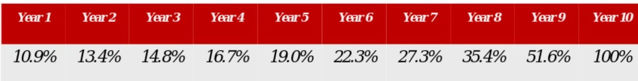
Year 1 Year 2 Year 3 Year 4 Year 5 Year 6 Year 7 Year 8 Year 9 Year 10

10.9% 13.4% 14.8% 16.7% 19.0% 22.3% 27.3% 35.4% 51.6% 100%

Table 3 - Percentage of CSM allocated at each reporting period

0 500 1 000 1 500 2 000 2 500 0 2 4 6 8 10 € Tho us ands Years

Behaviour of the CSM at initial recognition

Amount of CSM recognized in P&L Contractual Service Margin at Time t

For each case, the engine recalculated all future cash flows and the risk adjustment and updated the coverage units for the portfolio and corrected the allocation of the CSM. First, in the case of changes in the 3rd year:

The impact due to the number of deaths being higher than expected is reflected in the changes in fulfilment cash flows and it is equal to 567,606 €. Comparing to the CSM projection at initial recognition, the new behaviour of the CSM, due to the changes in the group of contracts, is reflected below.

0 50 100 150 200 250 300 1 2 3 4 5 6 7 8 9 10 € Tho us ands Year

Difference in the amount of CSM allocated on P&L

Initial Recognition After the third year

0 500 1 000 1 500 2 000 2 500 0 1 2 3 4 5 6 7 8 9 10 € Tho us ands Year

Behaviour of the CSM integrating changes in the 3rd_year

Finally, for the changes in the 6th year:

The impact due to the number of deaths being higher than expected is reflected in the changes in fulfilment cash flows and it is equal to 365,619 €. Comparing to all previous CSM projections, the new behaviour of the CSM, due to the changes in the group of contracts, is reflected below.

In the two cases, the CSM never turns negative and it runs-off until zero.

Consider a scenario where the CSM grows and then drops again. It was verified that the number of people that died in the portfolio was:

• In the 1st _{year, 1 person died instead of 13 and;} • In the 5 0 500 1 000 1 500 2 000 2 500 0 1 2 3 4 5 6 7 8 9 10 € Tho us ands Year

Behaviour of the CSM integrating changes in the 3rd_{and 6}th_year

Initial Recognition After the third year After the sixth year

0 50 100 150 200 250 300 1 2 3 4 5 6 7 8 9 10 € Tho us ands Year

Difference in the amount of CSM allocated on P&L

The evolution of the CSM allocation if the following:

During the run-off tail of the CSM, the amount allocated can became bigger than initially predicted, if proper conditions are applied. At the end of the 1st _{year, the CSM} had an increase of 292,108 €. At the end of the 5th year, it had a remarkable decrease of 1,217,159 €. The behaviour of the CSM, for the run, it is graphically represented below.

Even with the big drop that it suffer, due to the increase of more than 7 times the number of expected deaths in the 5th year, the CSM of the group of contracts absorbed the impact and remained positive in the end.

0 500 1 000 1 500 2 000 2 500 0 1 2 3 4 5 6 7 8 9 10 € Tho us ands Year

Behaviour of the CSM integrating changes in the 1st_{and 5}th_year

Initial recognition After the first year After the fifth year

0 50 100 150 200 250 300 350 1 2 3 4 5 6 7 8 9 10 € Tho us ands Year

Difference in the amount of CSM allocated on P&L

9 - Conclusions

For this new insurance standard, the CSM will be the centre of all groups of contracts within the entity’s portfolios, and most of the focus will be on the impacts that it might suffer throughout its run-off period.

As seen on this report, the group of contracts is profitable, if no significantly deviation arrives between reality and unexpected events. The CSM adjusts itself to any impact that it might encounter along the group of contracts coverage period. If the number of deaths is higher than expected, the CSM decreases, and if the number of deaths in lower than expected, the CSM increases, as showed.

The key point of this project was reached and it was possible to verify different behaviours for different scenarios, solely due to changes in the mortality assumption in the possible future events.

Some of the goals that were also meant to be done would involve more complex computations. For example, the higher the number of risks taking into consideration, the more challenging the RA gets and, not only to correlate all different risks, as talked in the Risk Adjustment chapter, but to determine all different distributions.

It is important to consider that the norm is still being discussed within insurance companies, consultants and all other entities that are reflecting about this new standard. Reflecting about, but not only, which approach should an entity consider for the interest rate and how to calculate the appropriated amount for each method, and which technique should be used for the RA.

With this report, the student was able to get, not only an overview of the standard, but also some practical experience of the working world.

A very simplified reality was pictured in this report, which is unlikely to happen. As such, there is plenty of room to improve what was done, for example: considering more risks and not only mortality, since life insurance contracts are expose to more than just death events; having a portfolio of assets and determining a more appropriate yield curve; and considering different contracts and different cohorts and not just an unique contract, to add more depth to the cash flows.

Bibliography

[1] EFRAG, Background briefing paper: IFRS 17 Insurance Contracts and Level of Aggregation (2018);

[2] EFRAG, Background briefing paper: IFRS 17 Insurance contracts and release of the contractual service margin (2018);

[3] EY, Applying IFRS 17: A closer look at the new Insurance Contracts Standard (2018); [4] EY, First technical discussion of the IASB’s IFRS 17 Transition Resource Group (TRG) (2018);

[5] Lieke-Rosa Koetsier, Optimising choices with respect to the risk adjustment in IFRS 17 (2018);

[6] KPMG, Insurance Contracts: First Impressions (2017);

[7] Thomas BEHAR, Hamdi KACEM, Approaches to evaluate Risk Adjustment under IFRS 17 (2019);

Annex

Value at Risk (VaR)

Let 𝐶𝐶 ∈ [0,1] be the confidence level, then let VaR of 𝐶𝐶 be 𝑉𝑉𝐷𝐷𝑅𝑅(𝐶𝐶): [0,1] → 𝐹𝐹−1(𝐶𝐶) where 𝐹𝐹 is the cumulative distribution function corresponding to the used distribution. This gives 𝐹𝐹�𝑉𝑉𝐷𝐷𝑅𝑅(𝐶𝐶)� = 𝐶𝐶. It follows that 𝑉𝑉𝐷𝐷𝑅𝑅(𝐶𝐶) can be calculated using

�𝑉𝑉𝑉𝑉𝑉𝑉(𝐶𝐶)𝑜𝑜(𝐸𝐸) 𝑐𝑐𝐸𝐸 = 𝐶𝐶 −∞

(6)

Conditional Tail Expectation (CTE)

Let 𝐶𝐶 ∈ [0,1] be the confidence level, and let the tail of the liability cash flows as the set of all values bigger than 𝑉𝑉𝐷𝐷𝑅𝑅(𝐶𝐶). Let 𝐶𝐶𝑇𝑇𝐵𝐵(𝐶𝐶): [0,1] → ℝ be the expected value of the tail, so

𝐶𝐶𝑇𝑇𝐵𝐵(𝐶𝐶) =_{1 − 𝐶𝐶 �}1 ∞ 𝑜𝑜(𝐸𝐸) ∙ 𝐸𝐸 𝑐𝑐𝐸𝐸 𝑉𝑉𝑉𝑉𝑉𝑉(𝐶𝐶)