ISSN: 1809-4430 (on-line) www.engenhariaagricola.org.br
2 Western Paraná State University/ Cascavel - PR, Brazil. 3 Paraná Federal Institute/ Foz do Iguaçu - PR, Brazil.
Received in: 3-9-2016
Doi:http://dx.doi.org/10.1590/1809-4430-Eng.Agric.v38n1p22-31/2018
STREAMFLOW REGIONALIZATION IN PIQUIRI RIVER BASIN
Fernanda C. Araujo
1*, Eloy L. de Mello
2, Gisele M. Gollin
2, Luciana E. de Quadros
3,
Benedito M. Gomes
21*Corresponding author. Western Paraná State University/ Cascavel - PR, Brazil. E-mail: [email protected]
KEYWORDS
water availability,
water resources
management, average
streamflow, low
flows, flows
permanence.
ABSTRACT
The objective of this study was to regionalize 7-day 10-year low flows, long-term annual
mean, and 90% and 95% permanence flows from Piquiri (PR) river basin. The following
regionalization methods were adopted: Traditional, Linear interpolation, Chaves,
Modified linear interpolation, and Modified Chaves. The equations obtained by the
Traditional method, adding main river length or drainage density as independent
variables, significantly improved R
2equations value. Streamflow forecasting by Linear
Interpolation and Chaves methods were as good as those provided by the Traditional
Method, thus, these methods could be applied to Piquiri River basin, especially when
drainage area is the only available spatial information.
INTRODUCTION
Streamflow data accuracy is of great importance for water resources planning and monitoring (Nruthya & Srinivas, 2015). Elesbon et al. (2015) described the need for good quality information, both in time and in space, for a proper and integrated management of water resources.
In hydrology, data are commonly gathered from hydrometric station networks, whose importance is proportional to the data-series time range (Costa & Fernandes, 2015). However, the limited availability of fluviometric data and the need to know the streamflow within a hydrographic network have impaired or, often, prevented a proper water resource management (Moreira & Silva, 2014). To overcome this problem, streamflow regionalization has often been employed (Reis et al., 2013).
The importance of streamflow regionalization is not only due to its capacity for spatializing hydrological information, but also because it can identify those areas in need for hydrometeorological network improvement, either by installing new stations or relocating the existing ones (Virões, 2013).
Despite all the efforts, there is still no single accepted approach for streamflow regionalization in river basins (Razavi & Coulibaly, 2013; Parajka et al., 2013).
The most commonly used regionalization methods are the regression-based approach, spatial proximity and physical similarity (Arsenault & Brissette, 2014).
In Brazil, Eletrobrás published a methodological guide, in 1985, presenting streamflow regionalization procedures, thus standardizing the technique, which became recognized as Traditional method or Eletrobrás method, used by several authors (Reis et al., 2013, Virões, 2013, Elesbon et al., 2015, Moreira & Silva, 2014).
Nevertheless, when available databases in a river basin are reduced, flows regionalization by this method presents great restrictions (Novaes et al., 2007). As most of the Brazilian river basins present lack of information, accuracy, and use of this regionalization method may not be recommended.
Some methods have been developed in order to overcome this limitation. Among them, we highlight the methodology based on Linear Interpolation, described by Eletrobrás (1985b), the method proposed by Chaves et al. (2002), and the modifications proposed by Novaes et al. (2007).
MATERIAL AND METHODS
Study area description
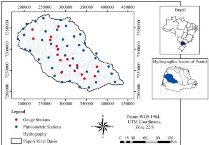
Piquiri River basin covers a drainage area of 24,156 km², which corresponds to 12.1% of the Paraná state borders (Figure 1), comprising totally 36 and partially 32 municipalities (SEMA, 2013), with an estimated population of 1,594,862 (IBGE, 2016), representing 14.2% of the total state.
Data selection, analysis, and processing
For this study, we used data from 18 stream and 48 rainfall gauge stations (Figure 1), which is part of Hydrological Information System (HidroWeb) hydrometeorological network, from National Water Agency (ANA).
Pluviometric data are from January 1980 to December 2010. Faults in the series were filled using regional weighting method, based on correlations with neighboring stations. For streamflow data, months presenting more than 5% of records without information were eliminated, and other faults were not completed.
FIGURE 1. Geographical location of Piquiri River basin - PR, with gauging and rainfall stations utilized in this study.
REGIONALIZATION METHODS
Traditional (T)
Following the procedure described by Eletrobrás (1985a), the Traditional method (T) was applied. Initially, for all the stations in the study region, i.e. considering the basin as a single homogeneous region, we tried to determine the best regression equation of the studied flows, contemplating selected physical and climatic characteristics of the river basin. Multiple regressions were applied among dependent and independent variables. Linear, potential, and simple or multiple exponential models were analyzed.
Regression models were selected based on the criteria of simplicity model and adjustment quality. Models, which disclosed concomitantly the following parameters, were compared with the other methods: a) lower residue; b) significant F-test results for the model; c) significant T-test results for the adjusted parameters; d) adjusted determination coefficient greater than 0.7.
Linear Interpolation (LI)
Once flow in the section of interest is obtained by proportionality relation between flows and drainage areas from the nearest gauging stations, Linear Interpolation method (LI) was applied (Eletrobrás, 1985b). The framing was necessary to apply the method, which relied on the relative position of the point of interest with regard to the nearest gauging stations, according to the four cases described below.
When the point of interest is located upstream (Case 1) or downstream (Case 2), [eq. (1)] estimated the desired flow.
(1)
where,
Q z = flow in the section of interest, m3s-1;
Qm, j = flow at upstream or downstream stations, m3 s-1;
Az = drainage area in the section of interest, km2,
Am, j = drainage area from upstream or downstream stations, km2.
When the point of interest is located in a stream section between two stream stations of known flow (Case 3), [eq. (2)] forecasts the incognito reference flow.
(2)
where,
Qm = flow at upstream station, m3s-1;
Q j= flow at downstream station, m3s-1;
Am= drainage area from upstream station, km2,
Aj= drainage area from downstream station, km2.
Case 4, however, is when the point is situated in a section of a tributary river whose mouth is located between two gauging stations, positioned in a higher order river. In this case, a combination of the two other situations described above is applied, streamflow being first calculated in confluence section, using [eq. (2)]. Then, streamflow within the section of interest is estimated using flows in the joining of rivers, by means of [eq. (1)].
Modified Linear Interpolation (LI-mod)
The Modified Linear Interpolation method (LI - mod) stemmed from an adaptation of Linear Interpolation method, from rainfall variable addition; in other words, it considers that streamflow in the section of interest has a direct and proportional relation to rainfall quantity in the respective contribution area (Novaes et al., 2007). Therefore, the eqs (1) and (2), used in Linear Interpolation method, are now expressed by eqs (3) and (4), respectively.
(3)
where,
Pz = annual mean rainfall in drainage area of the section of interest, mm;
Pm, j = annual mean rainfall in drainage area of upstream or downstream stations, mm;
Pm = annual mean rainfall in drainage area from upstream station, mm;
Pj = annual mean rainfall in drainage area from the downstream station, mm.
Chaves (C)
The method proposed by Chaves et al. (2002) (C) also presents four distinct situations, depending on the location of the section of interest regarding known flow sections, however, in addition to drainage areas, it considers the distances between the analyzed sections.
When the section of interest is located upstream (Case 1) or downstream (Case 2) from a stream station, the methodology is identical to Linear Interpolation, and thus, [eq. (1)] calculates streamflow in the section of interest. Yet in the case of point of interest being located in a canal section between two gauging stations, with known reference flow (Case 3), [eq. (5)] forecasts the incognito flow.
(5)
where,
(6) (7)
where,
pm = relative weight to the upstream station,
dimensionless; and
pj = relative weight to downstream station,
dimensionless.
dm = distance between the upstream station and
interest section, km;
dj = distance between the downstream station and
interest section, km.
As disclosed in Linear Interpolation method, the fourth situation (Case 4) occurs when interest section is located in a segment of a tributary river whose mouth is positioned between two gauging stations, settled in a higher order river. In this case, a combination of the two other situations described above was applied, in which the flow is first calculated in the confluence of rivers (Equation 5), and then, in the section of interest, using Equation 1.
Chaves modified (C - mod)
Based on Chaves et al. (2002) method, as well as in Modified Linear Interpolation method, this modification refers to rainfall variable insertion in the calculations, since it considers the rainfall influence on flow besides drainage area (Novaes et al., 2007). In this way, the eqs (1)
and (5), used in Chaves et al. (2002) method, are now expressed by eqs (3) and (8), respectively.
(8)
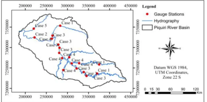
For Linear Interpolation (Eletrobrás, 1985b) application, Chaves et al. (2002) and their respective modifications, Modified Linear Interpolation and Modified Chaves, proposed by Novaes et al. (2007), firstly observing the basin map with stream stations plotted, each possible situation was identified in relation to the existing gauging stations (Figure 2).
Iporã station (64833000), located in a tributary river whose mouth is downstream of a fluviometric station – situation not described by the applied methods, was not framed in any case. Chaves et al. (2002) reported the need for diverse equations in basins other than that where the method was first used (Itapicuru basin), given their particularities (drainage network, stations distribution, etc.). In the case of Iporã station, here titled as Case 5, a combination of the already described cases was adopted. Primarily, Piquiri River flow at its mouth was calculated, selecting Case 2 equation, and then, applying Case 4 equations, Iporã station flow (64833000) was determined.
FIGURE 2. Framing of existing gauging stations prospects in Piquiri river basin (PR) in relation to the nearest stream gauge station.
Starting from source to mouth, Q7.10, Q90, Q95, and Qmed were determined for all gauging stations with known flow, whose flows were assumed unknown only for the purpose of testing, in a subsequent comparison among estimated flows values with other observed methods and values.
Dependent variables attainment
Independent variables attainment
The independent variables were obtained using ArcGIS 10 software and a Digital Elevation Model (MDE) from Paraná State, which was provided by the National Institute for Space Research (INPE), and offered as free access on TOPODATA project website, which resampled spatial resolution from 90 m to 30 m, on a 1: 250,000 scale.
Physical characteristics chosen for regionalization models construction were drainage area (A), main river length (Lp), main river slope between source and mouth (Sl), basin mean slope (Sm) and drainage density (Dd). Annual total rainfall (P) was the elected climatic characteristic (Table 1).
TABLE 1. Characteristics of sub-basins associated with gauging stations of Piquiri River basin.
Code* Name A
(km²)
Lp (km)
Dd (m km-²)
SI (m km-1)
Sm (%)
P (mm year-1)
64764000 Guampará 1687.5 151.4 0.71 3.58 14.68 1902.3
64765000 Paiquerê Harbour 3281.0 248.2 0.72 2.71 17.18 1900.1
64767000 Carriel Harbour 3536.4 261.1 0.72 2.64 17.38 1901.4
64771500 Guarani Harbour 4162.2 313.8 0.72 2.35 17.72 1904.1
64773000 Leôncio Primo Bridge 754.6 73.8 0.69 7.08 20.09 1993.5
64775000 Cantu Ferry 2521.0 184.4 0.69 3.61 16.62 1952.9
64776100 Cantu Mouth 7649.7 359.3 0.71 2.15 17.28 1918.2
64780000 Tourinho Bridge 274.3 34.8 0.63 7.14 10.71 1889.1
64785000 Goio-Bang Bridge 1335.3 134.1 0.64 3.46 8.64 1869.2
64790000 Salto Sapucaí 695.2 95.4 0.66 5.10 10.64 1799.2
64795000 Piquiri Bridge 11235.3 428.3 0.69 1.86 15.33 1895.2
64799500 New Port 2 12073.9 444.6 0.69 1.81 14.83 1893.9
64800000 Harbour 2 13100.4 454.2 0.68 1.78 14.19 1883.1
64810000 Goio-erê Ferry 2035.1 102.3 0.62 3.19 6.98 1719.0
64815000 Uberana Farm 2957.5 143.0 0.62 2.61 6.92 1688.4
64820000 Formosa Harbour 17415.9 501.3 0.67 1.65 12.39 1837.4
64830000 Santa Maria Ferry 20943.8 561.4 0.66 1.53 11.39 1824.3
64833000 Iporã 1065.5 60.6 0.62 3.03 7.73 1532.9
Notice: * Hidroweb Network Code / ANA; A = Drainage area; Lp = Main river length; Dd = Drainage density; Sl = Declivity between main river source and mouth; Sm = basin mean slope; P = annual total rainfall.
Annual total rainfall was obtained for each rainfall station, and then isohyets map was produced aiming to determine mean rainfall in drainage areas of the considered sub-basins. Isohyets were plotted using Interpolation method by inverse distance weighted squared (IDW).
Results comparison from different methods
The following indices were used as statistical indicators: a) relative error (ER) between obtained values from historical series analysis and regionalization methods (Equation 9); b) mean error (EM) (Equation 10); c) Nash and Sutcliffe efficiency criterion (NS) (Nash & Sutcliffe, 1970) (Equation 11); d) root mean square error (RMSE) (Equation 12); e) modified agreement Willmott et al. (2012) (dr) (Equation 13).
(9)
(10)
(11)
(12)
(13)
where,
= obtained flow from historical series
analysis (m³ s-1);
= estimated flow based on regionalization
methods (m³ s-1);
n = gauging stations number,
= observed flows mean (m³ s-1).
RESULTS AND DISCUSSION
Regionalization equations obtained by Traditional method
Table 2 reports the best regression equations selected for average flow forecast (Qmed), 7-day 10-year low flows (Q7.10), and 90% and 95% flows permanence (Q90 and Q95, respectively).
Drainage area (A) was the independent variable which contributed most to regression equations adjustment. Other authors, such as Elesbon et al. (2015), have already verified this result. Razavi & Coulibaly (2013), when reviewing regionalization methods, observed that, in general, drainage area is one of the attributes most used by the researchers.
TABLE 2. Selected equations to estimate minimum flows (Q7.10, Q90, and Q95), average flow rate (Qmed) in m³s-1 in Piquiri River basin.
Flow Model Equation* R² Simple
Potential 0.97
Simple
linear 0.86
Multiple
Potential 0.99
Simple
linear 0.94
Multiple
Potential 0.98
Simple
linear 0.92
Multiple
Linear 0.95
Notes: (*) A = Area (km²); Lp = main river length (m); Dd = drainage density (mkm-2).
Even so, the inclusion of main river length (Lp) improved the R2 value of the adjusted equations for Q
90 and Q95 forecasting; and the addition of drainage density (Dd) significantly enhanced the R2 value of the adjusted equation for Q7.10 assessment (Table 2).
In the case of Qmed (Table 2), the exponent value associated with drainage area was observed to be close to 1, causing the potential equation to present a similar result to a linear equation. This results in an approximately linear increase in average flow rate with drainage area upsurge, as described by Lisboa et al. (2008). Moreira & Silva (2014) also evidenced this fact when they regionalized flows in Paraopeba River basin. According to Eletrobrás (1985a), hydrological experience has highlighted the drainage area as the most important factor in mean flow calculation.
Comparison among methods
7-day 10-year low flows (Q7.10)
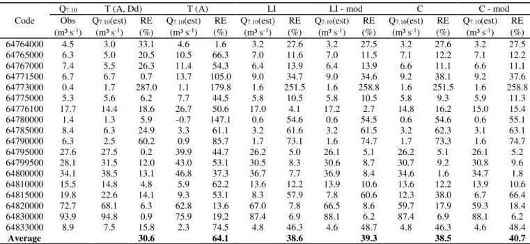
Table 3 discloses estimated values of 7-day 10-year low flows (Q7.10).
On average, the relative error in predictions performed by the Traditional Method, having only drainage area as an independent variable, was equal to 64.1%. Although, when regionalization equation was used with drainage area and drainage density as independent variables, relative error was equal to 30.6%, on average. Therefore, the inclusion of an independent variable in addition to drainage area, was important to improve equation adjustment (Table 2) and, consequently, to reduce relative error (Table 3).
TABLE 3. Q7.10 values, obtained from Log-Pearson 3 distribution analysis, Q7.10 estimated by the five evaluated methods (m³ s-1), and relative errors (RE).
Code
Q7.10 T (A, Dd) T (A) LI LI - mod C C - mod
Obs Q7.10(est) RE Q7.10(est) RE Q7.10(est) RE Q7.10(est) RE Q7.10(est) RE Q7.10(est) RE
(m³ s-1) (m³ s-1) (%) (m³ s-1) (%) (m³ s-1) (%) (m³ s-1) (%) (m³ s-1) (%) (m³ s-1) (%)
64764000 4.5 3.0 33.1 4.6 1.6 3.2 27.6 3.2 27.5 3.2 27.6 3.2 27.5 64765000 6.3 5.0 20.5 10.5 66.3 7.0 11.6 7.0 11.5 7.1 12.2 7.1 12.2 64767000 7.4 5.5 26.3 11.4 54.3 6.4 13.9 6.4 13.9 6.6 11.1 6.6 11.1 64771500 6.7 6.7 0.7 13.7 105.0 9.0 34.7 9.0 34.6 9.2 38.1 9.2 37.6 64773000 0.4 1.7 287.0 1.1 179.8 1.6 251.5 1.6 258.8 1.6 251.5 1.6 258.8 64775000 5.3 5.6 6.2 7.7 44.5 5.8 10.5 5.8 10.5 5.8 9.3 5.9 11.3 64776100 17.7 14.4 18.6 26.7 50.6 17.0 4.1 17.2 2.7 14.8 16.2 15.0 15.4 64780000 1.4 1.3 5.9 -0.7 147.1 0.6 54.6 0.6 54.5 0.6 54.6 0.6 55.1 64785000 8.4 6.3 24.9 3.3 61.1 3.2 61.6 3.2 61.5 3.2 62.3 3.1 63.1 64790000 6.3 2.5 60.2 0.9 85.7 1.7 73.1 1.6 74.7 1.7 73.3 1.6 74.7 64795000 27.6 27.5 0.2 39.9 44.7 26.2 5.0 26.1 5.1 26.2 5.1 26.1 5.2 64799500 28.1 31.5 12.0 43.0 53.1 30.5 8.3 30.6 8.7 30.7 9.2 30.8 9.6 64800000 34.1 38.5 13.1 46.8 37.3 36.7 7.7 36.9 8.4 34.6 1.6 34.7 1.8 64810000 15.5 14.8 4.8 5.9 62.2 13.6 12.2 13.9 10.6 13.6 12.2 13.9 10.6 64815000 19.8 22.6 14.1 9.3 53.1 8.3 57.9 7.8 60.6 12.3 38.0 6.7 66.4 64820000 72.7 68.1 6.3 62.8 13.6 67.0 7.8 66.5 8.6 59.7 17.9 59.3 18.4 64830000 93.9 94.8 0.9 75.9 19.2 87.4 6.9 88.1 6.2 87.4 6.9 88.1 6.2 64833000 8.9 7.5 15.8 2.3 74.5 4.8 46.3 4.6 48.7 4.8 46.3 4.6 48.4
Average 30.6 64.1 38.6 39.3 38.5 40.7
Notes: Q7.10 Obs = Low flow values (m3 s-1) associated with 10-years return period (Q7.10) according to Log-person distribution 3; T (A,
For the simple equation, the highest RE values in the Traditional method occurred in stations with smaller drainage areas and, consequently, smaller observed Q7.10 (Table 3), namely 64773000 (754.6 km²), 64790000 (695.2 km²) and 64780000 (274.3 km²). Novaes et al. (2007) report that, as relative error considers the observed value from historical series in the denominator (Equation 9), the smaller the denominator, the greater RE value tends to be. In Linear Interpolation (Eletrobrás, 1985b), Chaves et al. (2002) and their respective modifications, Modified Linear Interpolation and Modified Chaves methods, proposed by Novaes et al. (2007), mean relative errors were equal to 38.6; 38.5; 39.3 and 40.7%, respectively. It proves that, if the Traditional Method is applied with the support of more than one dependent variable, the relative error tends to be, on average, smaller than in other methods. On the other hand, if it is applied only with drainage area support, any of the other methods studied in this work should be preferably adopted.
For Linear Interpolation (Eletrobrás, 1985b), Chaves et al. (2002) and their respective modifications, Modified Linear Interpolation and Modified Chaves methods, proposed by Novaes et al. (2007), relative errors were also high in the station 64773000. In this case, though, following the required procedures for each of the methods, Q7.10 forecast for this station (64773000) was performed based on 64775000 station data. The relation between these two stations areas is equal to 3.34, whereas Eletrobrás (1985b) does not recommend a ratio higher than 3.0.
Table 4 shows the other utilized statistical indicators for regionalization flow methods evaluation for Q7.10 prediction in Piquiri river basin.
In the joint statistics analysis (Table 4) all the presented methods featured good results, but among them, the Traditional method (A, Dd) has the lowest RMSE value (2.39), and concordance (dr) and efficiency coefficient (NS) values closer to 1, 0.95 and 0.99,
respectively. Nevertheless, the Traditional method (A) was the opposite, holding the highest RMSE (8.94), and dr and NS values farther than 1.00, 0.78, and 0.92, respectively. Once again, drainage density inclusion into the Traditional method resulted in better forecasts than did with only drainage area.
TABLE 4. Statistical indicators: mean error (ME); Nash and Sutcliff efficiency ratio (NS); root mean square error (RMSE), and modified agreement of Willmott et al. (2012) (dr) from flows regionalization methods for Q7.10 prediction in Piquiri river basin.
T (A, Dd) T (A) LI LI - mod C C - mod ME 0.42 0.003 1.94 1.93 2.33 2.61
NS 0.99 0.92 0.97 0.97 0.97 0.96 RMSE 2.39 8.94 4.08 4.18 4.5 5.19 dr 0.95 0.78 0.91 0.91 0.91 0.9
Notes: T (A, Dd) = Traditional Method having drainage area (A) and drainage density (Dd) as independent variables; T (A) = Traditional Method having only drainage area (A); LI = Linear Interpolation; LI - mod = Modified Linear Interpolation; C = Chaves and C - mod = modified Chaves.
When comparing Linear Interpolation (Eletrobrás, 1985b), Chaves et al. (2002) and modifications, Modified Linear Interpolation and Modified Chaves methods — proposed by Novaes et al. (2007), we observed the preference for original methods over the others, mainly by RMSE analysis (Table 4).
90% and 95% flow permanence (Q90 and Q95)
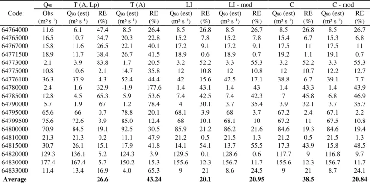
Tables 5 and 6 display the estimated values of 90% and 95% flow permanence (Q90 and Q95), obtained based on the methods used in this study.
TABLE 5. Relative error and 90% permanence of flow values (Q90), obtained by frequency classes method and estimated by the five evaluated methods (m³ s-1).
Code
Q90 T (A, Lp) T (A) LI LI - mod C C - mod
Obs Q90 (est) RE Q90 (est) RE Q90 (est) RE Q90 (est) RE Q90 (est) RE Q90 (est) RE
(m³ s-1) (m³ s-1) (%) (m³ s-1) (%) (m³ s-1) (%) (m³ s-1) (%) (m³ s-1) (%) (m³ s-1) (%)
64764000 11.6 6.1 47.4 8.5 26.4 8.5 26.8 8.5 26.7 8.5 26.8 8.5 26.7 64765000 16.5 10.7 34.7 20.3 22.8 15.2 7.8 15.2 7.8 15.4 6.7 15.3 6.8 64767000 15.8 11.6 26.5 22.1 40.1 17.2 9.1 17.2 9.1 17.5 11 17.5 11 64771500 18.9 11.7 38.4 26.7 41.5 18.9 0.6 18.9 0.7 19.2 1.1 19.1 0.7 64773000 2.1 3.9 83.8 1.7 20.5 3.2 52.2 3.3 55.3 3.2 52.2 3.3 55.3 64775000 10.8 10.6 2.1 14.7 35.8 12 10.8 12 10.8 12 10.7 12.2 12.7 64776100 36.3 37.9 4.3 52.4 44.4 42 15.6 42.5 17.1 38.8 6.7 39.1 7.7 64780000 2.4 1.6 32.9 -1.9 177.6 1.4 43.1 1.4 43 1.4 43.3 1.4 43.9 64785000 12.8 4.5 65.3 5.9 53.6 7.4 42.5 7.4 42.3 7 45.8 6.8 46.9 64790000 5.7 1.9 67 1.2 78.4 4 30.1 3.7 35.4 3.9 32.1 3.7 35.7 64795000 65.6 66 0.7 78.8 20.1 68.1 3.9 68 3.7 67.2 2.4 67.1 2.2 64799500 75.6 72.6 3.9 85.0 12.4 68 10.1 68.1 10 67.2 11 67.5 10.8 64800000 70.9 84.5 19.1 92.5 30.5 85.9 21.2 86.2 21.6 84.6 19.3 84.6 19.4 64810000 21.3 21.3 0.2 11.1 47.9 21.2 0.5 21.5 1.3 21.2 0.5 21.5 1.3 64815000 30.7 26.1 15.1 17.9 41.8 14.1 54.1 13.7 55.5 17.3 43.9 15.8 48.5 64820000 129.3 136.1 5.2 124.3 3.9 129.5 0.1 128.6 0.6 117.7 9 116.8 9.7 64830000 177.4 167.4 5.7 150.2 15.3 155.6 12.3 156.7 11.7 155.6 12.3 156.7 11.7 64833000 11.4 13.4 16.9 4.0 65.3 9 21 8.6 24.5 9 21 8.7 24.1
Average 26.6 43.24 20.1 20.95 38.5 20.84
Notes: Obs = 90% flow permanence (Q90) obtained from historical series analysis; T (A, Lp) = Traditional Method having drainage area (A)
For 90% flow permanence (Table 5), relative error forecasts, performed by the Traditional method (A), were observed to be equal to 43.24%, on average. However, relative error reduced to 26.6%, when carrying out estimations by the Traditional method (A, Lp). Thus, the inclusion of an independent variable, main river length, and drainage area, was important to improve equation adjustment (Table 2) and, consequently, to reduce relative error (Table 5).
In general, Linear Interpolation (Eletrobrás, 1985b), Modified Linear Interpolation and Modified Chaves methods, proposed by Novaes et al. (2007), obtained the lowest mean relative errors, being 20.1; 20.95 and 20.84%, respectively (Table 5), all of them even lower than in the Traditional method (A, Lp).
For Linear Interpolation (Eletrobrás, 1985b), Chaves et al. (2002) and their respective modifications, Modified Linear Interpolation and Modified Chaves
methods, proposed by Novaes et al. (2007), as well as in Q7.10 forecasts, the highest RE values occurred at 64773000 station, either for Q90 (Table 5) and Q95 (Table 6).
The largest relative errors were noticed in the Traditional method (A, Lp) for Q95, 518.745 and 409.63%,
being respectively observed in 64773000 and 64780000 stations (Table 6), which have relatively small areas when compared to the other stations: 754.75 and 272.73 km², correspondingly. Other authors, such as Moreira & Silva (2014), have already demonstrated this relation of high RE values for stations close to headwaters. For these authors, this behavior is associated with the greater natural regularization of the basins with larger drainage area. Thus, bigger variations in flow rates for small basins can be expected. Therefore, the Traditional method application for small drainage areas refers to the need for a careful analysis in flow forecasts use.
TABLE 6. Relative error and 95% flow permanence values (Q95), obtained by frequency classes method and estimated by the five evaluated methods (m³ s-1)
Code
Q95 T (A, Lp) T (A) LI LI - mod C C - mod
Obs Q95 (est) RE Q95 (est) RE Q95 (est) RE Q95 (est) RE Q95 (est) RE Q95 (est) RE
(m³ s-1) (m³ s-1) (%) (m³ s-1) (%) (m³ s-1) (%) (m³ s-1) (%) (m³ s-1) (%) (m³ s-1) (%)
64764000 8.9 5.7 36.4 6.6 26.2 6.6 26.1 6.6 26 6.6 26.1 6.6 26 64765000 12.8 6.4 49.6 16.0 25.1 11.9 6.6 11.9 6.7 12.1 5.6 12.1 5.7 64767000 12.4 7 43.8 17.5 41.4 12.7 2.2 12.7 2.2 13.3 6.9 13.3 6.9 64771500 12.5 5 59.7 21.2 69.9 14.8 18.7 14.8 18.5 15 20.2 15 19.8 64773000 1.4 8.4 518.7 1.0 26.1 2.5 84.2 2.5 88 2.5 84.2 2.5 88 64775000 8.3 8.8 5.1 11.5 38.7 9.3 11.6 9.3 11.6 9.2 10.8 9.2 10.8 64776100 28.2 32.2 14 41.9 48.7 30.2 7 30.6 8.5 26.9 4.7 27.2 3.8 64780000 1.9 9.7 409.6 -1.8 195.4 1.1 43.8 1.1 43.7 1.1 44 1.1 43.9 64785000 9.5 4.9 48.9 4.5 52.9 5.5 41.8 5.5 41.6 5.3 44.3 5.3 44.4 64790000 4.8 4.5 6.2 0.7 85.8 3 38.2 2.8 42.5 2.9 39.5 2.8 42.7 64795000 48.4 56.8 17.2 63.2 30.5 49.1 1.5 49.1 1.3 48.6 0.4 48.6 0.3 64799500 54 62.5 15.6 68.2 26.2 52.3 3.3 52.4 3 52.3 3.2 52.5 2.9 64800000 56.9 71.1 24.8 74.2 30.5 64.5 13.3 64.8 13.8 62.5 9.8 62.6 9.9 64810000 19.5 16.6 14.9 8.6 55.8 18.4 5.5 18.7 3.8 18.4 5.5 18.7 3.8 64815000 26.8 19.4 27.6 14.1 47.4 13 51.4 12.3 54.1 12.8 52.3 12.7 52.4 64820000 108.3 106.1 2.1 99.8 7.8 105.3 2.8 104.5 3.5 95.3 12 94.7 12.6 64830000 144.8 131.4 9.2 120.8 16.6 130.3 10.1 131.2 9.4 130.3 10.1 131.2 9.4 64833000 10.9 13.5 22.6 2.9 73.6 7.4 32.8 7 35.9 7.4 32.8 7.1 35.5
Average 73.7 49.9 22.7 23.0 22.9 23.3
Notes: Obs = 95% flow permanence (Q95) obtained from historical series analysis; T (A, Lp) = Traditional Method having drainage area (A) and main river length (Lp) as independent variables; T (A) = Traditional Method having only drainage area (A) as independent variable; LI = Linear Interpolation; LI- mod = Modified Linear Interpolation; C = Chaves and C - mod = Modified Chaves.
In general, for the 95% flow permanence by the Traditional method (Table 6), the relative error went from 49.9%, in forecasts performed using drainage area (A), until 73.7%, in assessments using both drainage area and main river length (A, Lp). Therefore, the inclusion of main river length independent variable contributed to the improvement in equation adjustment (Table 2), but not to relative error reduction, since relative mean error increased to 23.8% (Table 6).
Linear Interpolation (Eletrobrás, 1985b), Chaves et al. (2002) and their respective modifications, Modified Linear Interpolation and Modified Chaves methods, proposed by Novaes et al. (2007), obtained the lowest mean relative errors, being 22.7, 23, 22.9 and 23.3%, respectively (Table 6). Thus, the methods can be applied to Piquiri River basin, especially when the only available spatial information is drainage area.
All the methods seemed adequate, although, by joint statistics analysis (Table 7), Traditional method is verified to be the one allowing better forecasts of 90% flows permanence (Q90), since it obtained the lowest RMSE value of 5.72, and concordance (dr) and efficiency (NS) rates closer to 1, being 0.94 and 0.98, respectively.
TABLE 7. Statistical indicators: mean error (ME), Nash and Sutcliffe efficiency criterion (NS), root mean square error (RMSE), and correlation coefficient by Willmott et al. (2012) (dr) of flow regionalization methods for estimating Q90 in Piquiri river basin.
T (A, Lp) T (A) LI LI - mod C C - mod ME 1.53 -0.00047 1.9 1.88 2.72 1.9 NS 0.98 0.94 0.97 0.97 0.97 0.97 RMSE 5.72 11.32 47.93 7.87 7.91 7.93 dr 0.94 0.87 0.93 0.93 0.93 0.93
Notes: T (A, Lp) = Traditional Method having drainage area (A) and main river length (Lp) as independent variables; T (A) = Traditional Method having only drainage area (A) as independent variable; LI = Linear Interpolation; LI - mod = Modified Linear Interpolation; C = Chaves and C - mod = Modified Chaves.
The accuracy of estimated values in relation to observed data, evaluated through concordance (dr) and efficiency (NS) rates, point out as the most efficient method for estimating 95% flow permanence rate (Q95) the Linear interpolation, for presenting 0.94 and 0.98 values, respectively (Table 8). RMSE value, which informs about model accuracy, was also verified to present the lowest variation in Linear Interpolation method.
TABLE 8. Statistical indicators: mean error (ME), Nash and Sutcliffe efficiency criterion (NS), root mean square error (RMSE), and correlation coefficient by Willmott et al. (2012) (dr) of flow regionalization methods for estimating Q95 in Piquiri river basin.
T (A, Lp) T (A) LI LI - mod C C - mod ME 0.04 -0.02 1.81 1.81 2.67 2.63 NS 0.97 0.92 0.98 0.98 0.97 0.97 RMSE 6.98 10.8 5.39 5.42 6.07 6.04 dr 0.90 0.84 0.94 0.94 0.93 0.93
Notes: T (A, Lp) = Traditional Method having drainage area (A) and main river length (Lp) as independent variables; T (A) = Traditional Method having only drainage area (A) as independent variable; LI = Linear Interpolation; LI - mod = Modified Linear Interpolation; C = Chaves and C - mod = Modified Chaves.
Average flow rate (Qmed)
Table 9 discloses relative errors percentage (%), calculated among average long-term flows (Qmed), obtained from historical series analysis and those estimated by the studied methods from Piquiri river basin gauging stations.
The relative errors of Qmed forecasts were smaller if compared to those of Q7.10, Q90, and Q95, ranging from 65.9% at 64833000, with the Traditional method, to 0.8% at 64776100, with the Modified Chaves (Table 9). Such performance was also evidenced by Novaes et al. (2007) and Moreira & Silva. (2014). For these authors, this behavior is associated with the fact that Qmed values, since are medium and non-extreme flow rates, disclose a lower magnitude variation in comparison with the other flows.
On average, the relative error in predictions performed by the analyzed methods (Table 9) reported very close values, ranging from 19.8% for the Traditional method to 17.65% for Modified Chaves method (proposed by Novaes et al., 2007), which corresponds to 2.15% on average.
TABLE 9. Average streamflows (Qmed) from historical series (from annual average flow) estimated by the five evaluated methods (m³ s-1), and respective relative errors (RE).
Code
Qmed(est) T (A) LI LI - mod C C - mod
Obs Qmed(est) RE Qmed(est) RE Qmed(est) RE Qmed(est) RE Qmed(est) RE
(m³ s-1) (m³ s-1) (%) (m³ s-1) (%) (m³ s-1) (%) (m³ s-1) (%) (m³ s-1) (%)
64764000 53.8 48.4 10.0 41.7 22.5 41.7 22.4 41.7 22.5 41.7 22.4 64765000 81.1 90.1 11.1 101.1 24.8 101.1 24.7 101.2 24.9 101.1 24.8 64767000 108.7 96.6 11.1 92.5 14.9 92.5 14.9 89.7 17.5 89.8 17.4 64771500 120.5 112.5 6.6 125.5 4.2 125.4 4.1 123.3 2.3 122.9 2.0 64773000 29.6 22.8 22.9 19.9 32.9 20.3 31.5 19.9 32.9 20.3 31.5 64775000 66.4 70.4 6.1 72.3 8.9 72.3 8.9 72.3 8.9 72.3 8.9 64776100 219.4 198.6 9.5 210.6 4.0 212.8 3.0 215.6 1.7 217.5 0.8 64780000 6.5 8.9 37.2 7.7 19.3 7.7 19.4 7.7 19.4 7.7 19.5 64785000 29.6 38.9 31.3 36.7 23.7 36.7 24.0 37.3 26.0 37.3 25.8 64790000 17.8 21.2 18.7 18.8 5.7 18.0 0.9 19.0 6.7 18.0 1.0 64795000 303.3 284.3 6.3 333.6 10.0 333.3 9.9 332.9 9.8 332.3 9.6 64799500 360.4 304.1 15.6 281.0 22.0 280.1 22.3 267.8 25.7 268.6 25.5 64800000 253.6 328.1 29.4 371.8 46.6 372.1 46.7 378.3 49.2 377.8 49.0 64810000 45.4 57.7 27.0 42.2 7.1 43.0 5.4 42.2 7.1 43.0 5.4 64815000 61.3 81.8 33.4 23.6 61.6 27.7 54.8 79.5 29.7 79.5 29.7 64820000 420.0 428.0 1.9 397.2 5.4 395.0 6.0 377.0 10.2 373.8 11.0 64830000 514.6 508.5 1.2 505.0 1.9 508.7 1.1 505.0 1.9 508.7 1.1 64833000 19.0 31.5 65.9 26.2 37.7 25.0 31.5 26.2 37.7 25.1 32.3
Average 19.8 19.62 18.41 18.46 17.65
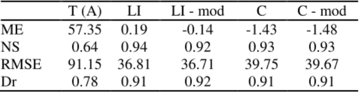
Table 10 shows the other statistical indicators used for regionalization flow methods evaluation for QMed forecast in Piquiri river basin.
In statistical indicators analysis (Table 10), the analyzed methods were verified to have obtained close performances, nevertheless, Linear Interpolation method and its modification stand out, that is, the methods obtained the lowest EM and RMSE errors and concordance and efficiency rates closer to 1. Yet, Modified Linear Interpolation method application requires the inclusion of rainfall variable, that is, it entails a greater difficulty in applying the methodology, as agreed by Novaes et al. (2007).
TABLE 10. Statistical indicators: mean error (ME), Nash and Sutcliffe efficiency criterion (NS), root mean square error (RMSE), and correlation coefficient by Willmott et al. (2012) (dr) of streamflow regionalization methods for estimating Qmed in Piquiri river basin.
T (A) LI LI - mod C C - mod ME 57.35 0.19 -0.14 -1.43 -1.48
NS 0.64 0.94 0.92 0.93 0.93
RMSE 91.15 36.81 36.71 39.75 39.67
Dr 0.78 0.91 0.92 0.91 0.91
Notes: T (A) = Traditional Method having only drainage area (A) as independent variable; LI = Linear Interpolation; LI - mod = Modified Linear Interpolation; C = Chaves and C - mod = Modified Chaves.
In general, the Modified Linear Interpolation and Modified Chaves methods, proposed by Novaes et al. (2007), did not provide significant improvements to be recommended, in view of the harm to the method by including rainfall as variable.
As a recommendation, we suggest other studies using the Traditional method with more than one independent variable in regression equations, mainly for Q7.10 and Q90 flows, which obtained a good improvement with an independent variable inclusion, in addition to drainage area.
Both Linear Interpolation and Chaves et al. (2002) methods could also be suggested for other river basins with lower densities of gauging stations, once the advantage of these methods lies exactly in situations where there is limited information, as quoted by Novaes et al. (2007).
CONCLUSIONS
The Traditional method generated equations, using the drainage area (A) as an independent variable, which was adequate for minimum and average streamflow forecasts. Conversely, when either the main river length (Lp) or drainage density (Dd) was added as variables, R2 increased, mainly for predictions of 7-day 10-year low flows.
Streamflow forecasting by Linear Interpolation and Chaves methods were as good as those provided by the Traditional one, thus, they could then be used for predictions in the Piquiri River basin, especially when drainage area is the only available spatial information.
Both the Modified Linear Interpolation and Modified Chaves methods, proposed by Novaes et al.
(2007), did not promote significant improvement in streamflow estimations if compared to the originals.
ACKNOWLEDGMENTS
Our thanks to CAPES, for the financial support to this research.
REFERENCES
Arsenault R, Brissette FP (2014) Continuous streamflow prediction in ungauged basins: the effects of equifinality and parameter set on uncertainty in regionalization approaches. Water Resources Research 50(7):6135-6153.
Chaves HML, Rosa JWC, Vadas RG (2002)
Regionalização de vazões mínimas em bacias através de interpolação em sistemas de informação geográfica. Revista Brasileira de Recursos Hídricos 7(3):43-51.
Costa KT, Fernandes WS (2015) Avaliação do tipo de distribuição de probabilidade das vazões máximas diárias anuais do Brasil. Revista Brasileira de Recursos Hídricos 20(2):442-451.
Elesbon AAA, Silva DD da, Sediyama GC, Guedes HAS, Ribeiro CAAS, Ribeiro CB de M (2015) Multivariate statistical analysis to support the minimum streamflow regionalization. Engenharia Agrícola 35(5):838-851.
Eletrobrás (1985a) Metodologia para regionalização de vazões. Eletrobrás, 212p.
Eletrobrás (1985b) Manual de minicentrais hidrelétricas. Eletrobrás, p46-47.
GPRH - Grupo de Pesquisa em Recursos Hídricos (2008) SisCAH 1.0 - Sistema computacional para análises hidrológicas. (Programa computacional).
IBGE - Instituto Brasileiro de Geografia e Estatística (2016) Estimativas da população residente para os
municípios e para as unidades da federação brasileiros com data de referência em 1º de julho de 2016. Available: http://www.ibge.gov.br/home/estatistica/populacao/estimat iva2016/estimativa_dou.shtm. Accessed Jul 23, 2017.
Lisboa L, Moreira MC, Silva DDda, Pruski FF (2008) Estimativa e regionalização das vazões mínimas e média na bacia do rio Paracatu. Engenharia na Agricultura 16(4):471-479.
Moreira MC, Silva DD (2014) Análise de métodos para estimativa das vazões da Bacia do Rio Paraopeba. Revista Brasileira de Recursos Hídricos 19(2):313-324.
Nash JE, Sutcliffe JV (1970) River flow forecasting through conceptual models, Part I - A discussion of principles. Journal of Hydrology 10:282-290.
Novaes LFde, Pruski FF, Queiroz DO de, Rodriguez R del G, Silva DD da, Ramos MM (2007) Avaliação do
desempenho de cinco metodologias de regionalização de vazões. Revista Brasileira de Recursos Hídricos 12(2):51-61.
Razavi T, Coulibaly P (2013) Classification of Ontario basins based on physical attributes and streamflow series. Journal of Hydrology 18(8):958-975.
Reis JAT dos, Caiado MAC, Barbosa JF, Moscon M, Mendonça ASF (2013) Análise regional de vazões mínimas de referência na região centro-sul do estado do Espírito Santo. Revista de Ciências Exatas Aplicadas e Tecnológicas 5(2):1-11.
Parajka J, Viglione A, Rogger M, Salinas JL, Sivapalan M, Bloschl G (2013) Comparative assessment of predictions in ungauged basins - Part 1: Runoff-hydrograph studies. Hydrology and Earth System Sciences 17(5):1783-1795.
SEMA - Secretaria de Estado do Meio Ambiente e Recursos Hídricos (2013) Bacias hidrográficas do Paraná. SEMA, 2ed. 140p.
Virões MV (2013) Regionalização de vazões nas Bacias Hidrográficas Brasileiras: estudo da vazão de 95% de permanência da sub-bacia 50 – Bacias dos rios Itapicuru, Vaza Barris, Real, Inhambupe, Pojuca, Sergipe,
Japaratuba, Subaúma e Jacuípe. Recife, Companhia de Pesquisa de Recursos Minerais. 154p.