Aplicação de método pseudo-dinâmico no estudo da flexão de vigas sob carga transiente

(1)

Aplicação de método pseudo-dinâmico no estudo da flexão

de vigas sob carga transiente

Leonardo Miguel Brás da Costa

Dissertação de Mestrado

Orientador na FEUP: Prof. Pedro Moreira e Prof. Francisco Melo

Mestrado Integrado em Engenharia Mecânica

(2)

(3)

Resumo

O método pseudo-dinâmico é um procedimento híbrido, em que o resultado obtido por um algoritmo que simula o comportamento dinâmico de uma estrutura leva a deslocações em cada passo que são prescritos para a estrutura com a utilização de um atuador e a força de restauro medida pela célula de carga é alimentada ao algoritmo que lhe permite calcular os deslocamentos para o passo seguinte. Desta forma, a não-linearidade das estruturas pode ser contabilizada.

O método foi aplicado para determinar a resposta de uma barra de alumínio e de uma barra de Teflon sujeitas a cargas transversais transientes. A barra de Teflon foi testada considerando que não há amortecimento viscoso no algoritmo numérico. A barra de alumínio foi sujeita a dois testes: um sem considerar amortecimento viscoso, e outro considerando um quarto do amortecimento crítico. Isto foi concretizado com o algoritmo OS, baseado no método Newmark, e com o instrumento de teste Instron E1000.

Através do algoritmo OS, obteve-se respostas semelhantes a modelos analíticos e observa-se o efeito da não-linearidade na rigidez de uma estrutura real.

(4)

Application of the pseudo-dynamic method in the study of bending

of beams under a transversal load

Abstract

The pseudo-dynamic method is a hybrid procedure, where the result obtained by an algorithm simulating the dynamic behaviour of a structure leads to displacements in each time step that are prescribed to the structure with the use of an actuator and the restoring force measured by the load cell is fed into the algorithm which then allows it to calculate the displacements for the next step. This way, the non-linearity of structures can be accounted for.

The method was applied to determine the response of an aluminum bar and a Teflon bar that were subjected to transversal transient loads. The Teflon bar was tested considering no viscous damping in the numerical algorithm. Two tests were performed with the aluminum bar: one considering no viscous damping, and another considering one fourth of critical damping. This was accomplished with the OS algorithm, based on the Newmark method, and with the Instron E1000 test instrument.

Through the OS algorithm, responses similar to analytical models were obtained and the effects of non-linearity in the stiffness of a real structure were observed.

(5)

Agradecimentos

Agradeço ao Prof. Pedro Moreira e ao Prof. Franciso Melo por me orientarem na tese. Agradeço também à minha família e amigos por me apoiarem nesta jornada.

(6)

1 Introduction

1.1 Background

The pseudo-dynamic test combines a numerical technique with restoring forces obtained experimentally. It was first implemented by Takanashi, Udagawa et al. (1975), which they called the "computer-actuator on-line system", to evaluate the seismic performance of structures under earthquake-induced loading.

The method has been developed along the years. Recently, Chang and Kim (2019) used the pseudo-dynamic method to analyze the response of a multi-degree of freedom structural system with the effect of soil-structure interaction being taken into account. Wang, Pan et al. (2019) investigated end plate moment‑resisting CFST frames. Terzic and Stojadinovic (2014) evaluated the traffic performance of a highway overpass bridge after a major earthquake by physically testing one of the columns through substructuring. Chu, Lu et al. (2018) investigated the non-linearity of semi-active control device through real-time hybrid testing by using a shaking table.

Non-linear hysteresis loops such as bi-linear, tri-linear, Ramberg-Osgood type, etc. have been used for analytical models of the earthquake response analysis of structures, it is necessary to develop more realistic analytical models that can represent the stiffness and strength deterioration of the structure during an earthquake. Simplified analytical models might not be able to represent the real non-linearity of structures, which depend on unpredictable factors such as non-linearity of materials, local failures, loss of structural stability, etc. (Takanashi, Udagawa et al. 1975). The pseudo-dynamic test method measures the actual restoring forces of the structures, thus does not require analytical stiffness models.

Although the most direct method for structures under seismic loading, the shaking table test, offers a realistic option to account for the non-linear dynamic history of structures, it also comes with limitations. When using a shaking table test, the structure is placed upon the test floor. The test floor then reproduces the ground motion present in earthquakes with the help of actuators connected to the floor. However, shaking tables have a limitation in the size, weight and strength of the structure that can be tested. Tables designed to test larger scale structures have high costs. Because the pseudo-dynamic test is performed with a lower rate of loading, it requires less actuator capacity to displace large scale structures.

The pseudo-dynamic method is based on a discrete-parameter model with a finite number of degrees of freedom (DOF) (Takanashi, Udagawa et al. 1975, Pan, Wang et al. 2016). As such, the equation of motion can be expressed as:

𝑀𝑎𝑡_{+ 𝐶𝑣}𝑡_{+ 𝑟}𝑡_{= 𝑓}𝑡 _(1.1)

where M and C are the mass and damping matrices of the system, respectively, 𝑎𝑡 and 𝑣𝑡 are the nodal acceleration and velocity of the system at the time instant 𝑡, r is the restoring force vector, and 𝑓𝑡 is the external excitation at the time instant t. For a linear elastic system, 𝑟 = 𝐾𝑑, where K is the stiffness matrix and d is the nodal displacement vector.

1.2 Implementation

Time integration algorithms compute a displacement step based on the equation of motion, which is then imposed on the structure by actuators. At the consequent displacement, a load cell will measure the restoring force of the structure which is then fed back into equation (1.1).

(8)

For “Ramp and Hold”, while the displacement is on “hold”, data acquisition and numerical computations are carried out. The hold period leaves room for force relaxation, which combined with the sudden change of velocity between “hold” and “ramp” introduces errors to the response. This is especially undesirable for real-time pseudo-dynamic tests (Mahin and Shing 1985, Mosalam and Günay 2013).

The “Continuous Loading” method does not have these issues. During the prediction stages, the actuator moves on a predicted trajectory based in previous computed displacements. When the computation is concluded, the actuator moves to the computed displacement during the correction stage (Mosalam and Günay 2013). It requires a control loop for the actuators of only a few milliseconds to obtain smooth actuator motion (Pavese, Le Maoult et al. 2012).

1.3 Advantages

The pseudo-dynamic test has advantages over quasi-static tests and numerical analysis. Since the pseudo-dynamic test measures restoring forces directly from the specimen, it can simulate the complex non-linearity of a structure without requiring a numerical model. Pseudo-dynamic tests also simulate the seismic responses of structures unlike the quasi-static test which can only investigate the load capacity of structures.

Pseudo dynamic tests have been carried out on an expanded time scale. Since dynamic effects are simulated numerically, the displacements can be applied at any rate or even be stopped and restarted. This requires less actuator capacity and allows the use of conventional measuring devices. In fact, pseudo-dynamic tests can be performed with quasi-static test equipment. It also allows for larger structures, since it’s not limited by the capacity of shaking tables (Pan, Wang et al. 2016).

1.4 Constraints

Despite having efficient means for experimental research, pseudo-dynamic tests come with limitations as well. It is not possible to model continuum structures that require refined spatial discretization to yield accurate results. Since only a limited amount of degrees of freedom can be controlled by actuators, the method relies on discretizing the structure with masses and springs. The testing of continuous structures might require a large number of actuators, which discourages the use of this method. In addition, the viscous damping properties are assigned arbitrarily, so the method is not desirable if viscous damping has a high influence on the response of the structure and there is not an accurate numerical model for it.

The rate of loading should be considered. For some materials, its strength is lower with a lower rate of loading. Thus, a quasi-static rate of loading might yield a lower structural resistance. Furthermore, the failure mechanism may depend on the rate of loading (Pan, Wang et al. 2016).

1.5 Errors in pseudo-dynamic tests

Errors can be attributed to experimental errors, errors due to structural modeling and numerical errors.

The restoring forces meant to be feedback to the numerical algorithm is prone to experimental errors due to a presence of a transfer system (controllers, actuators, reaction systems, and data acquisition systems). Experimental errors can occur during the application of the displacement or the measurement of the restoring force. Experimental errors can be either random or systematic. Random errors are difficult, if not impossible to be predicted. They may arise from random electrical noise in electrical components. Experimental errors have a greater effect on higher modes of vibration. Therefore, random noise in the measured force can excite an inaccurate response in high frequency modes. Systematic errors are caused by specific

(9)

phenomena that lead to error propagation and numerical instability. Errors in the measurements, techniques for applying displacements (such as ramp and hold, continuous or real-time) and in servo-hydraulic closed control loop are the systematic error sources. The source of measurement errors can be mechanical, electrical or human related. Progress in digital measurement technology is helping reduce measurement errors (Mosalam and Günay 2013).

1.6 Substructuring (hybrid testing)

One of the features that make pseudo-dynamic testing so versatile is the ability to test a portion of a structure and model numerically the remaining part. Tests of full-scale models can be expensive and require large facilities, so physically testing only the most critical substructures can prove to be useful (Darby, Blakeborough et al. 1999).

Typically, with actuators, displacements are applied to the experimental substructure and the restoring forces are measured. The number and configuration of actuators depend on the interface boundary conditions between experimental and analytical substructures (Mosalam and Günay 2013).

1.7 Real time pseudo-dynamic test

Normal pseudo-dynamic tests use loadings at slow rates for simulations where the rate of loading is negligible. However, for rate-dependent materials, a real-time pseudo-dynamic test is necessary. It makes use of either actuators for discrete degrees of freedom or a shaking table. Nakashima, Kato et al. (1992) proposed this system by introducing a dynamic actuator, a digital displacement transducer and a digital servomechanism. The digital servomechanism guarantees accurate displacement and velocity control.

Bayer, Dorka et al. (2005) performed a real-time pseudo-dynamic test of a payload mounted into a carrier rocket.

1.8 Thesis objective and structure

The objective of this dissertation was to determine the response of beams subjected to transversal transient loads, using the pseudo-dynamic method.

With that in mind, the thesis was structured as follows:

Chapter 2 – Different algorithms that can be used for the pseudo-dynamic test are listed. It details the methodology of each one and the respective limitations.

Chapter 3 – Numerical examples are performed to validate some of the algorithms mentioned in Chapter 2. These examples include different loading conditions and the effect of plasticity on a structure, which an algorithm must be able to account for.

Chapter 4 – Pseudo-dynamic tests are applied to different specimens that are displaced by an actuator. The results are discussed and compared with analytical solutions.

Chapter 5 – Final remarks and findings on the subject are discussed. Afterwards, some options for future research are considered.

(10)

2 Time integration algorithms for pseudo-dynamic test

As mentioned in chapter Error! Reference source not found., the pseudo-dynamic method r elies on solving the equations of motion (2.1) using time integration algorithms.

𝑀𝑎𝑡+ 𝐶𝑣𝑡+ 𝑟𝑡= 𝑓𝑡 (2.1)

Newmark Method:

The Newmark method (Newmark 1959) is the most widely used family of time integration methods. It uses two parameters, β and γ, to indicate how much of the acceleration at the end of the time interval enters into the relations for velocity and displacement at the end of the time interval. 𝑀𝑎𝑡+∆𝑡+ 𝐶𝑣𝑡+∆𝑡+ 𝑟𝑡+∆𝑡 = 𝑓𝑡+∆𝑡 (2.2) 𝑣𝑡+∆𝑡_{= 𝑣}𝑡_{+ [(1 − 𝛾)𝑎̈}𝑡_{+ 𝛾𝑎}𝑡+∆𝑡_]∆𝑡 _(2.3) 𝑑𝑡+∆𝑡 = 𝑑𝑡+ ∆𝑡𝑣𝑡+ [(1 2− 𝛽) 𝑎 𝑡_{+ 𝛽𝑎}𝑡+∆𝑡_{] ∆𝑡}2 (2.4) For 𝛽 = 0 and 𝛾 =1

2, the algorithm is similar to the central difference method. As such, the

stability condition is ∆𝑡 <𝑇𝑛

𝜋. Typical time steps are ∆𝑡 = 𝑇𝑛

10.

For 𝛽 =1

4 and 𝛾 = 1

2, it is called the average acceleration method and it is unconditionally

stable.

HHT-α Method:

The Hilber Hughes Taylor (HHT)-α method improves the numerical dissipation of the Newmark method by introducing the parameter α to the stiffness and damping terms of the equation of motion as formulated in equation (2.5) (Pan, Wang et al. 2016).

𝑀𝑎𝑡+∆𝑡+ (1 + 𝛼)𝐶𝑣𝑡+∆𝑡− 𝛼𝐶𝑣𝑡+ (1 + 𝛼)𝑟𝑡+∆𝑡− 𝛼𝑟𝑡 = (1 + 𝛼)𝑓𝑡+∆𝑡− 𝛼𝑓𝑡 (2.5) 𝑣𝑡+∆𝑡= 𝑣𝑡+ [(1 − 𝛾)𝑎𝑡+ 𝛾𝑎𝑡+∆𝑡]∆𝑡 (2.6) 𝑑𝑡+∆𝑡 = 𝑑𝑡+ ∆𝑡𝑣𝑡+ [(1 2− 𝛽) 𝑎 𝑡_{+ 𝛽𝑎}𝑡+∆𝑡_{] ∆𝑡}2 (2.7) Where 𝛽 =1 4(1 − 𝛼) 2_{and 𝛾 =} 1 2− 𝛼.

The method is unconditionally stable for −1

3< 𝛼 < 0.

For 𝛽 ≠ 0, the system of equations (2.2) - (2.4) of the Newmark method and the system of equations (2.5) - (2.7) of the HHT-α method are implicit in the sense that the displacement in the next step, 𝑑𝑡+∆𝑡, can only be calculated after the restoring force, 𝑟𝑡+∆𝑡, is known but the restoring force can only be known after the displacement 𝑑𝑡+∆𝑡 is imposed on the structure. If the procedure were purely numerical, the equations could be solved by iteration, such as with the Newton-Raphson method. However, since the experimental structure is sensitive to the response history, iterations will apply an artificial response, which would be inexistent the real dynamic response (Mosalam and Günay 2013).

(11)

2.1 Explicit methods

For 𝛽 = 0 and 𝛾 =1

2, the Newmark algorithm is similar to the central difference method.

Replacing 𝑑𝑡+∆𝑡 and 𝑣𝑡+∆𝑡 in equation (2.2) and with 𝛽 = 0 and 𝛾 = 1

2, the equations

(2.2)-(2.4) can be re-written as:

𝑎𝑡+∆𝑡 = (𝑀 +∆𝑡 2 𝐶) −1 (𝑓𝑡+∆𝑡_{− 𝑟}𝑡+∆𝑡_{− 𝐶𝑣}𝑡₋∆𝑡 2 𝐶𝑎 𝑡₎ (2.8) 𝑣𝑡+∆𝑡 _{= 𝑑}𝑡₊∆𝑡 2 (𝑎 𝑡_{+ 𝑎}𝑡+∆𝑡₎ (2.9) 𝑑𝑡+∆𝑡 _{= 𝑑}𝑡_{+ ∆𝑡𝑣}𝑡₊∆𝑡 2 2 𝑎 𝑡 (2.10)

In this form, the displacement in the next step is obtained with the values of the displacement, velocity and acceleration from the previous step, then the displacement is applied to the structure, then the restoring force is fed into equation (2.8) to solve the acceleration and then the velocity. As such, it’s an explicit method. It doesn’t require iterations.

2.2 Implicit methods 2.2.1 Analogue feedback

Thewalt and Mahin (1987) were the first to use an implicit algorithm. They used the HHT-α method, although it can be applied to any implicit method. The displacements were expressed as: 𝑑𝑡+∆𝑡= 𝑑𝑡+ ∆𝑡𝑣𝑡+ (1 2− 𝛽) ∆𝑡 2_𝑎𝑡_{+ 𝛽∆𝑡}2_𝑀−1_(𝑓𝑡+∆𝑡_{+ 𝛼𝑟}𝑡₎ + 𝛽∆𝑡2𝑀−1(1 + 𝛼)𝑟𝑡+∆𝑡 (2.11)

Equation (2.11) can be separated by the explicit part where all the variables are known and the implicit part which contains 𝑟𝑡+∆𝑡 as is shown in Equation (2.12).

𝑑𝑡+∆𝑡 = 𝑑₀𝑡+∆𝑡+ 𝐺𝑟𝑡+∆𝑡 (2.12)

There is a relationship between analogue and digital representations of displacement and the restoring forces.

𝑑 = 𝐺𝑑𝑉𝑑 (2.13)

𝑟 = 𝐺𝑟𝑉𝑟 (2.14)

Then the command signal, 𝑉_𝑑 for the displacement can be written as:

𝑉_𝑑 = 𝐺_𝑑−1(𝑑₀𝑡+∆𝑡+ 𝐺𝐺_𝑟𝑉_𝑟) (2.15) Given the command signal, as the displacement is being applied by the servo-controllers, the restoring values change in function of the current displacement and feedback 𝑉𝑟 to equation

(2.15), therefore updating the command signal to account the most recent restoring force. Despite its perfect feedback mechanism, it is hard to implement due to the hardware requirements.

(12)

2.2.2 Digital feedback

As an alternative to analogue feedback, the restoring force can be fed back digitally over discrete substeps, where the explicit part may be applied linearly.

Using Equation (2.12) as an example, to apply the substeps it is written as: 𝑑_𝑖𝑡+∆𝑡 ≈ [(1 − 𝑖 𝑘) 𝑑0 𝑡 ₊ 𝑖 𝑘𝑑0 𝑡+∆𝑡_{] + 𝐺𝑟} 𝑖−1𝑡+∆𝑡(𝑑𝑖−1𝑡+∆𝑡) (2.16)

Where i is the iteration number and k is the number of substeps.

2.2.3 Polynomial extrapolation

Chang and Kim (2019) predict the acceleration for the next time step 𝑡 + ∆𝑡 by employing an extrapolation scheme using the previous acceleration responses. The third order polynomial function is used, since for higher orders the increase in accuracy is not enough to compensate the computational cost.

𝑎(𝑖) = 4𝑎(𝑖 − 1) − 6𝑎(𝑖 − 2) + 4𝑎(𝑖 − 3) − 𝑎(𝑖 − 4) (2.17) Where 𝑎(𝑖) is the extrapolated acceleration for the next time step 𝑡 + ∆𝑡. It corresponds to 𝑎𝑡+∆𝑡.

The first three predictions are performed with constant, first order and second order, respectively:

𝑎(1) = 𝑎(0) (2.18)

𝑎(2) = 2𝑎(1) − 𝑎(0) (2.19)

𝑎(3) = 3𝑎(2) − 3𝑎(1) + 𝑎(0) (2.20)

2.2.4 OS method

OS-method (also known as operator splitting method) is based on the implicit-explicit method (Hughes, Pister et al. 1979), the stiffness is divided into a linear part and a nonlinear part. The explicit predictor-corrector method is employed for the nonlinear stiffness and the HHT-α method is applied to the linear stiffness.

Predictor displacement:

𝑑̃𝑡+∆𝑡 _{= 𝑑}𝑡_{+ ∆𝑡𝑣}𝑡_{+ (}1

2− 𝛽) ∆𝑡

2_𝑎𝑡 (2.21)

Equation of motion based on the HHT- α method:

𝑀𝑥̈𝑡+∆𝑡_{+ (1 + α)𝐶𝑥̇}𝑡+∆𝑡_{− α𝐶𝑥̇}𝑡_{+ (1 + α)𝑟}𝑡+∆𝑡_{− α𝑟}𝑡

= (1 + α)𝑓𝑡+∆𝑡 _{− α𝑓}𝑡 (2.22)

where 𝑟𝑡+𝛥𝑡(𝑑𝑡+𝛥𝑡_{) ≈ 𝐾}𝐼_𝑑𝑡+𝛥𝑡_{+ 𝑟̃}𝑡+𝛥𝑡_(𝑑̃𝑡+𝛥𝑡_{) − 𝐾}𝐼_𝑑̃𝑡+𝛥𝑡

The correction for the displacement is given as:

𝑑𝑡+∆𝑡 = 𝑑̃𝑡+∆𝑡 + 𝛽∆𝑡2𝑎𝑡+𝛥𝑡 (2.23)

and velocity is given as:

𝑣𝑡+∆𝑡 = 𝑣𝑡+ 𝛥𝑡(1 − 𝛾)𝑎𝑡+ 𝛥𝑡𝛾𝑎𝑡+𝛥𝑡 (2.24) The process is to

(13)

• calculate the predictor displacement • apply the displacement to the structure • read the restoring force

• solve for 𝑑𝑡+∆𝑡_{, 𝑣}𝑡+∆𝑡_{and 𝑎}𝑡+∆𝑡_{with equations (2.22)-(2.24)} 2.2.5 Incremental Pseudo-Dynamic Method

The temporal evolution of displacement, velocity and acceleration vectors of the dynamic loaded structure is in each time step registered as:

𝑑𝑡+∆𝑡 = 𝑑𝑡+ 0.5𝛥𝑡(𝑣𝑡+ 𝑣𝑡+𝛥𝑡)

𝑣𝑡+∆𝑡 _{= 𝑣}𝑡_{+ 0.5𝛥𝑡(𝑎}𝑡_{+ 𝑎}𝑡+𝛥𝑡₎ (2.25)

Equations (2.25) can be re-written as 𝑣𝑡+∆𝑡 ₌ 2 𝛥𝑡(𝑑 𝑡+𝛥𝑡_{− 𝑑}𝑡_{) − 𝑣}𝑡 𝑎𝑡+∆𝑡 ₌ 2 𝛥𝑡(𝑣 𝑡+𝛥𝑡_{− 𝑣}𝑡_{) − 𝑎}𝑡 (2.26)

Replacing the equations (2.26) into the equation of motion (2.1), gives: 𝑟𝑡+𝛥𝑡_{+ (}2𝑐 𝛥𝑡+ 4𝑚 𝛥𝑡2) 𝑑𝑡+𝛥𝑡 = 𝑓𝑡+𝛥𝑡+ ( 2𝑐 𝛥𝑡+ 4𝑚 𝛥𝑡2) 𝑑𝑡+ (𝑐 + 4𝑚 𝛥𝑡) 𝑣 𝑡_{+ 𝑚𝑎}𝑡 (2.27)

Assuming a linear behavior for within a time step, the restoring forces and displacements for the time step 𝑡 + 𝛥𝑡 can be written as:

𝑟𝑡+𝛥𝑡 = 𝑟𝑡+ ∆𝑟 𝑑𝑡+𝛥𝑡 = 𝑑𝑡+ ∆𝑑

(2.28) Introducing tangential flexibility, which is the inverse of tangential rigidity, the relationship between increments of restoring forces and displacements can be expressed as:

∆𝑑 = 𝐶_𝑡∆𝑟 (2.29)

where 𝐶_𝑡 is the tangential flexibility.

Inserting equations (2.28)-(2.29) into equation (2.27) leads to the equation for incremental restoring force: (1 +2𝐶𝑡𝑐 𝛥𝑡 + 4𝐶_𝑡𝑚 𝛥𝑡2 ) 𝛥𝑟 = 𝑓 𝑡+𝛥𝑡_{− 𝑟}𝑡_{+ (𝑐 +}4𝑚 𝛥𝑡) 𝑣 𝑡_{+ 𝑚𝑎}𝑡 _(2.30)

Equation (2.30), where all the variables in the right-side member are known, must be solved for 𝛥𝑟

Knowing 𝛥𝑟, the restoring force for the next time step is obtained:

𝑟𝑡+𝛥𝑡 _{= 𝑟}𝑡_{+ ∆𝑟} _(2.31)

That force is then applied to a specimen with the help of an actuator and the consequent displacement 𝑑𝑡+𝛥𝑡 is measured and sent back to the algorithm.

Then 𝐶𝑡 can be calculated:

(14)

The procedure repeats for the next time step.

2.3 Conclusion

This chapter introduced time integration algorithms to solve the equations of motion of pseudo-dynamic tests as well as implementation methods.

The Newmark method is self-started and unconditionally stable with a specific parameter. The HHT-α method improves on the numerical dissipation of the Newmark method.

Explicit algorithms are easy to implement into pseudo-dynamic tests but are conditionally stable. Stability is only guaranteed until a maximum time interval.

Implicit algorithms are unconditionally stable, but it is harder to implement given that it requires iterative methods that might introduce loading different from the pretended response.

The next chapter will validate the Central Difference Method, OS Method and Incremental Pseudo-Dynamic Method.

(15)

3 Numerical examples

Some of the algorithms in Chapter 2 will be validated by numeric examples. The algorithms tested in the first example are the CDM algorithm (Central Finite Method) the OS algorithm, and the INCREP (Incremental Pseudo-Dynamic Method in the Generalized Dynamic Analysis of Structures) algorithm, while the following examples will use only the OS algorithm. The first example features a theoretical structure with constant stiffness to compare the response with the analytical solution, while the second example features a theoretical structure with a non-linear force-displacement relationship to test if the algorithms can calculate the consequent response. The third example covers bending with axial forces.

3.1 Example 1 — Linear stiffness

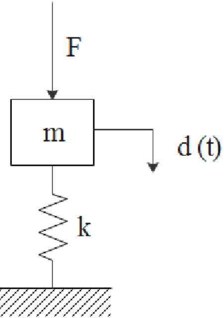
For simplicity sake, the first example will be a simple mass-spring system with 1 DOF under a constant step force of 10 N. The system consists of a mass of 1 kg and a linearly elastic spring with a rigidity of 1000 N/m and thus a flexibility of 0.001 m/N.

Figure 3.1 - Spring-mass model

According to Rodrigues (2016) the analytical solution of this problem for an initial displacement of 𝑥(𝑡 = 0) = 0 is known as:

The experimental part will be simulated numerically on this example. Where the relationship between the restoring forces and displacements is linear.

For the OS algorithm, the consequent restoring force due to the prescribed displacement is given as:

𝑟_{𝑚𝑒𝑎𝑠𝑢𝑟𝑒𝑑} = 𝑘𝑑_{𝑝𝑟𝑒𝑠𝑐𝑟𝑖𝑏𝑒𝑑} (3.2)

And likewise, for the INCREP algorithm:

𝑑_{𝑚𝑒𝑎𝑠𝑢𝑟𝑒𝑑} = 𝐶_𝑡𝑟_{𝑝𝑟𝑒𝑠𝑐𝑟𝑖𝑏𝑒𝑑} (3.3) 𝑥(𝑡) =𝐹

(16)

The natural frequency is known to be 𝜔_n = √𝑘

𝑚= 31.623 rad/s and consequently the natural

period is T_n = 0.2 s. For a good resolution of the response, the time step chosen must be lower than the natural period. Thus, the time step was arbitrarily chosen as ∆t = 0.01 s.

The initial parameters of the example are listed in Table 1. The external force is established in Equation (3.4).

Table 1 - Initial parameters

k(N/m) 1000 m (kg) 1 c (Ns/m) 0 ωn (rad/s) 31.623 Tn (s) 0.2 Δt (s) 0.01 r0 (N) 0 d0 (mm) 0 v0 (m/s) 0 a0 (m/s2) 10

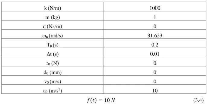
Figure 3.2 shows the response calculated analytically and numerically with the INCREPS method, the OS method and CDM. The results of INCREPS and OS are nearly the same. The three methods appear to have similar results with the analytical response, specially the CDM algorithm. The amplitude of the responses for all methods seems to be approximately the same of 20 mm, although, compared to the analytical response, CDM appears to have a slightly lower period while INCREPS and OS have a higher period.

Figure 3.3 shows the force-displacement relationship of the analytical response and all the numerical responses. As established, the relationship is linear.

(17)

Figure 3.2 – Response of the system using the analytical solution, the CDM method, the INCREPS method and the OS method.

(18)

3.2 Example 2 — Bilinear hysteresis model

The system will be the same as in Example 1, however now it will be simulated a non-linear behavior of the specimen, particularly with a bi-linear model.

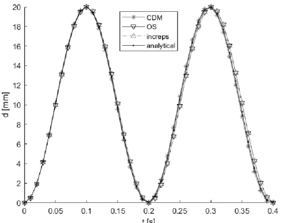
The force-displacement curve will behave linearly with a rigidity of 1000 N/m tangential until it reaches the yield load of 15 N. Then from there, the growth is linear, however with 100 N/m tangential rigidity, as presented in Figure 3.4.

It is represented by the expression. 𝐹(𝑑) = { 𝑘1𝑑, 𝑑 < 𝐹𝑦𝑖𝑒𝑙𝑑/𝑘1 𝑘2𝑑 + (1 − 𝑘₁ 𝑘2 ) 𝐹_{𝑦𝑖𝑒𝑙𝑑}, 𝑑 ≥ 𝐹𝑦𝑖𝑒𝑙𝑑/𝑘1 (3.5) Where: 𝑘₁ = 1000 𝑁/𝑚 𝑘₂ = 100 𝑁/𝑚 𝐹𝑦𝑖𝑒𝑙𝑑 = 15 𝑁

For a decrease in displacement, the relationship is linear. The displacement due to plastic deformation is 𝑑_𝑝 = 𝑑 − 𝐹/𝑘₁

Figure 3.4 – Force-displacement curve as expressed by equation (3.5)

Using the OS method, the response and force-displacement relationships were obtained as presented in, respectively, Figures 3.5 and 3.6.

The obtained displacement due to plastic deformation was 𝑑_𝑝 = 6.7 𝑚𝑚. Adding that to the static displacement of 𝑑_𝑠 = 10 𝑚𝑚 the estimated equilibrium displacement is of 𝑑 = 16.7 𝑚𝑚 which seems to correspond to the response in Figure 3.5.

(19)

This example demonstrates that the pseudo-dynamic method can calculate the responses of structures working in the plastic regime.

(20)

3.3 Example 3 — Bending with axial forces (push-over)

Generally, in constructions, bending is caused by seismic transversal forces. Constructions are designed to support mostly the effect of transversal forces, however the effect of compression forces on columns supporting building stories are a permanent load due to the weight of the structure.

The effect of axial forces can increase the bending moment in beam-columns because of the increase of deflection due to transversal forces.

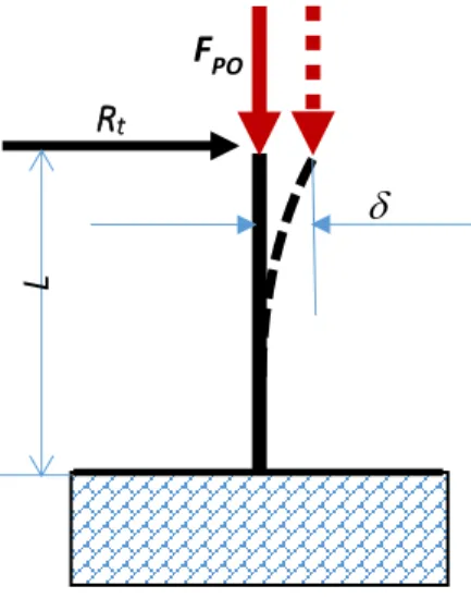
A virtual system will be developed to simulate the effect of axial forces on bending. The specimen will be subjected to a permanent axial load that interacts with the bending moment caused by the transversal force as illustrated in Figure 3.7.

Figure 3.7 - Transversal bending of the beam with "push-over"

Where Rt is the restoring force. The beam is subjected to two bending moments:

• The moment due to the transversal force Rt

• The moment due to the compression force Fpo

The two forces induce a transversal displacement . The displacement is established as proportional to the equivalent moment defined in Equation (3.6).

𝑀_𝑒𝑞= 𝑅_𝑡𝐿 + 𝐹_𝑝𝑜𝛿 (3.6)

Given that the compliance of this structure in the linear-elastic regime is defined in Equation (3.7) as:

𝐶_𝑡 = 𝐿

3

3𝐸𝐼

(3.7) Then the displacement can be expressed as Equation (3.8). By re-writing Equation (3.8) as restoring force in function of displacement, it becomes Equation (3.9). Thus, the stiffness of the structure can be established as in Equation (3.10).

𝛿 =𝑅𝑡𝐿 3 3𝐸𝐼 + 𝐹_𝑝𝑜𝛿𝐿2 3𝐸𝐼 (3.8) 𝑅_𝑡 = 3𝐸𝐼 𝐿3 (1 − 𝐹_𝑝𝑜𝐿2 3𝐸𝐼 ) 𝛿 (3.9)  Rt F_PO L

(21)

𝑘 =3𝐸𝐼 𝐿3 (1 −

𝐹_𝑝𝑜𝐿2

3𝐸𝐼 ) (3.10)

In the particular case of the compression force in Equation (3.11), the stiffness in Equation (3.10) becomes zero, which means it is under critical buckling load with an effective length factor of K=2, according to Euler’s theory (Timoshenko and Gere 1985). The critical load of a free-fixed column is described in Equation (3.12).

𝐹𝑝𝑜 =

3𝐸𝐼

𝐿2 (3.11)

𝐹_{𝐶𝑟𝑖𝑡}= 2.47𝐸𝐼

𝐿2 (3.12)

The difference between Equations (3.11) and (3.12) comes from the assumption that the displacement is proportional to the bending moment, even though for a triangular bending moment along the length of the beam results in transversal displacements along the length of the beam that follow a cubic function. To correct this discrepancy, the stiffness in Equation (3.10) is re-written as Equation (3.13) where the critical buckling load is now as Equation (3.12).

𝑘 =3𝐸𝐼 𝐿3 (1 −

𝐹_𝑝𝑜𝐿2

2.47𝐸𝐼) (3.13)

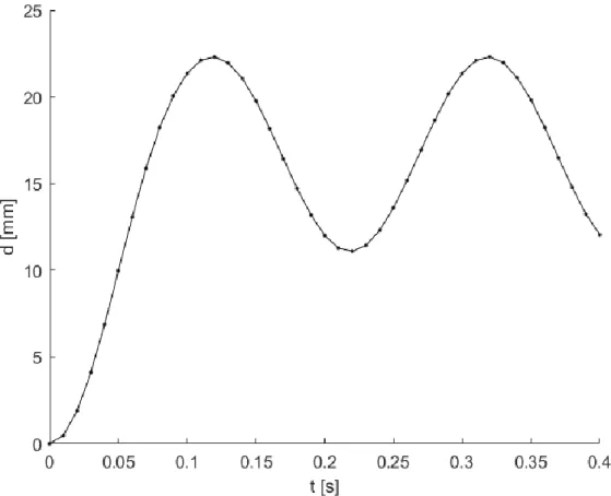
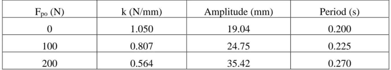
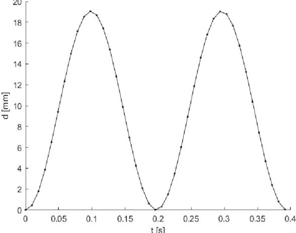
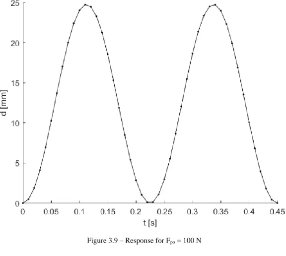
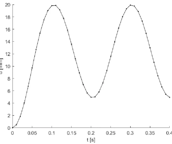
Pseudo-dynamic tests were performed numerically, assuming the stiffness in Equation (3.13). The initial parameters are presented in Table 2. Three tests were made with different compressive forces which results are presented in Table 3 and Figure 3.8, Figure 3.9 and Figure 3.10. The increase of the compression force results in a decrease of stiffness and consequently and increase in the displacement and the period.

Table 2 – Initial parameters

E (GPa) 210 I (mm4) 208.333 L (mm) 500 m (kg) 1.02 c (Ns/mm) 0 Δt (s) 0.01 r0 (N) 0 d0 (mm) 0 v0 (m/s) 0 a0 (m/s2) 10

Table 3 – Amplitude and period of response for different values of compressive force

Fpo (N) k (N/mm) Amplitude (mm) Period (s)

0 1.050 19.04 0.200

(22)

Two more tests were performed with a simulated plastic deformation defined as the tangential stiffness being halved if the restoring surpasses 15 N. The results are presented from Figure 3.11 to Figure 3.14.

(23)

(24)

Figure 3.11 - Response for Fpo = 0 N, with plasticity

(25)

(26)

4 Experiments

Experiments were performed to test the accuracy of the pseudo-dynamic method and if it is suitable for dynamic analysis.

The experiments featured specimens subject to a 3-point bending configuration by an Instron ElectroPuls E1000 actuator. The supports holding the specimen have a spacing of 16 mm. The setup is shown in Figure 4.1.The static capacity and stroke of the actuator are detailed in Table 4.

Table 4 - Instron ElectroPuls E1000 specifications

Static capacity (N) ±710

Stroke (mm) 60

The simulation must take into account the limitations of the actuator. The simulation again will be of a step force caused by the weight of a mass placed upon the center of a beam. The system’s single DOF is the deflection of the center of the beam.

Just as in Chapter 3, the system is numerically modeled with 1 DOF and a concentrated mass in the middle.

According to Rodrigues (2016) the damped response to a step force is known as

Where 𝜉 is the damping ratio and 𝜔𝑑 is the damped natural frequency. These are defined

respectively in Equations (4.2) and (4.3).

The maximum displacement is x𝑚𝑎𝑥 = 2𝐹/𝑘. Then the maximum restoring force is r𝑚𝑎𝑥 =

𝑘𝑥𝑚𝑎𝑥 = 2𝐹. The static capacity of the actuator is of ±710 N. As such the step force cannot be

greater than 355 N, which corresponds to the weight of a mass of 36.2 kg.

Due to the construction of the experiment, it is only possible to bend the specimen downward and not upward. To avoid the actuator seizing contact with the beam, the test must be set up as to not result in responses near or below zero. As such, the test will simulate two concentrated masses: mass 1 at rest with the beam that provokes a static displacement of the beam, and mass 2 will be dropped onto the beam to induce vibration. The response is then:

Where 𝐹1is the weight of mass 1 and 𝐹2 is the weight of mass 2.

Table 5 displays the weights that have been arbitrarily chosen for the masses as well as the corresponding masses.

Table 5 – Weights and masses

𝐹₁ [N] 50 𝑚₁ [kg] 5.1 𝐹₂ [N] 300 𝑚₂ [kg] 30.6 𝐹_{𝑡𝑜𝑡𝑎𝑙} [N] 350 𝑚_{𝑡𝑜𝑡𝑎𝑙} [kg] 35.7 𝑥(𝑡) =𝐹 𝑘[1 − 𝑒 −𝜉𝜔𝑛𝑡_{(cos 𝜔} 𝑑𝑡 + 𝜉 √1 − 𝜉2sin 𝜔𝑑𝑡)] (4.1) 𝜉 = 𝑐 2𝑚𝜔_𝑛 (4.2) 𝜔_𝑑 = 𝜔_𝑛√1 − 𝜉2 (4.3) 𝑥(𝑡) =𝐹1 𝑘 + 𝐹2 𝑘 [1 − 𝑒 −𝜉𝜔𝑛𝑡_{(cos 𝜔} 𝑑𝑡 + 𝜉 √1 − 𝜉2sin 𝜔𝑑𝑡)] (4.4)

(27)

The maximum restoring force is then 𝐹₁+ 2𝐹₂ = 650 𝑁 which is below the maximum capacity of the actuator.

The external excitation after mass 2 contacts the beam is defined in Equation (4.5).

Three tests have been performed:

• Test 1 – Aluminium specimen, no simulated damping. • Test 2 – Aluminium specimen, with simulated damping. • Test 3 – Teflon specimen, no simulated damping.

The hysteretic energy dissipation will be calculated for Test 1 and Test 3. It is defined as:

Where 𝑑𝑖 and 𝑑𝑖+1 are the displacements for the 𝑖th and 𝑖 + 1 th time step, respectively. 𝑟𝑖 and

𝑟_𝑖+1 are the corresponding restoring forces, respectively.

𝑓(𝑡) = 350 𝑁 (4.5) 𝐸ℎ = ∑ 1 2(𝑟𝑖+1+ 𝑟𝑖)(𝑑𝑖+1− 𝑑𝑖) 𝑛 𝑖=0 (4.6)

(28)

(29)

4.1 Test 1

The specimen is a 34x250x15 mm aluminum bar and the length between the two points supporting it is 16 mm long. It weighed 0.116 kg. The test used the OS algorithm. The test was performed with no simulated damping. The initial parameters used for the algorithm are featured in Table 6.

Table 6 - Initial parameters of test 1

k0 (N/mm) 221 m (kg) 35.7 c (Ns/mm) 0 ωn (rad/s) 78.7040 Tn (s) 0.080 Δt (s) 0.005 r0 (N) 50 d0 (mm) 0.232 v0 (m/s) 0 a0 (m/s2) 8.4086

The response of the test is shown in Figure 4.2. It also features an analytical response with an assumed rigidity of 252 N/mm, obtained by performing a linear regression of the force-displacement relationship of the test seen in Figure 4.3. The hysteretic energy dissipation is of 0.068 J.

The response is approximately sinusoidal with not much deviation from the analytical response since the behaviour of the bar is almost linearly elastic. A slight plastic deformation is observed. The difference between the analytical and experimental responses are listed in Table 7.

Table 7 – Characteristics of the response

Method Period (s) Amplitude (mm)

Maximum displacement

(mm)

Analytical 0.0748 2.38 2.61

(30)

Figure 4.2 – Response of aluminium specimen without viscous damping

(31)

4.2 Test 2

Experiment 2 repeats experiment 1 with the same specimen, except damping is now considered to be one fourth of critical damping. Furthermore, the initial displacement and initial rigidity must be measured again, due to possible plastic deformation from the previous experiment. Consequently, the estimated natural frequency and period have been recalculated, although the difference is negligible, thus the time step will be the same.

Table 8 – Initial parameters of test 2

k0 (N/mm) 216 m (kg) 35.7 c (Ns/mm) 1.3880 ωn (rad/s) 77.8086 Tn (s) 0.081 Δt (s) 0.005 r0 (N) 50 d0 (mm) 0.262 v0 (m/s) 0 a0 (m/s2) 8.4086

The response of the test is shown in Figure 4.4. It also features an analytical response with an assumed rigidity of 248 N/mm, obtained by performing a linear regression of the force-displacement relationship of the test seen in Figure 4.5.

The response shows a decrease in amplitude, similar to the analytical response. The difference between the analytical and experimental responses are listed in Table 9.

Table 9 - Characteristics of the response

Method Period (s) Maximum displacement

(mm)

Analitic 0.0778 2.037

(32)

Figure 4.4 - Response of aluminium specimen with viscous damping

(33)

4.3 Test 3

The specimen is a 92x250x10 mm Teflon bar and the length between the two points supporting it is 16 mm long. It weighed 0.780 kg. The test used the OS algorithm. The test was performed with no simulated damping. The initial parameters used for the algorithm are featured in Table 10.

Table 10 - Initial parameters of test 3

k0 (N/mm) 98.5 m (kg) 35.7 c (Ns/mm) 0 ωn (rad/s) 52.5435 Tn (s) 0.12 Δt (s) 0.01 r0 (N) 50 d0 (mm) 0.405 v0 (m/s) 0 a0 (m/s2) 8.4086

The response in Figure 4.6 shows a decrease in amplitude despite there being no viscous damping in the simulation. This is due to the structural damping of the material. The hysteretic energy dissipation is of 0.3855 J, thus the effects of hysteresis are more sever in the Teflon specimen in comparison with the aluminium specimen.

(34)

Figure 4.6 - Response of Teflon specimen

(35)

5 Conclusions and future research

The pseudo-dynamic method involves a hybrid procedure, where the result obtained by an algorithm simulating the dynamic behaviour of a structure leads to displacements in each time step that are prescribed to the structure with the use of an actuator and the restoring force measured by the load cell is fed into the algorithm which then allows it to calculate the displacements for the next step.

In the version known as the direct method, the displacements are prescribed to the structure and the cell charges register the internal restoring forces. When a structure has high stiffness, within a linear elastic regime, the force-displacement relationship approximately resembles Figure 5.1.

Figure 5.1 – Force-displacement in a linear elastic regime

What can be observed is that a deviation in prescribed displacements result in a much higher number of the restoring force. For example, if the displacement transducer has a resolution of 0.01 mm and the stiffness is 105_{N/m, the deviation in the restoring forces is of 1 N, while if the}

stiffness is 106 N/m, the deviation is of 10 N. Cell charges generally have extensometers carrying an analog signal to an analog-to-digital converter. This equipment can have a resolution inferior to 1 N, thus the errors are introduced into the algorithm due to the reading of displacements rather than the reading of the forces.

The OS algorithm has been used to perform pseudo-dynamic tests, simulating the drop of a mass onto a bar. The OS algorithm is shown to output responses similar to analytical models and accounts for the non-linearity in stiffness of a real structure.

Future research will involve integrating the computer algorithm with an actuator, for more controlled results. Due to limitations, the displacements had to be applied manually in the actuator for every time step. This thesis only explored 1 degree of freedom, thus higher degrees of freedom could be explored, either by the use of more actuators or substructuring. The effect of compressive forces on real beams should be tested with the pseudo-dynamic method. Different impact velocities should also be tested. Finally, more practical applications of the pseudo-dynamic test should be explored.

U R

(36)

References

Bayer, V., U. E. Dorka, U. Füllekrug and J. Gschwilm (2005). "On real-time pseudo-dynamic sub-structure testing: algorithm, numerical and experimental results." Aerospace Science and Technology 9(3): 223-232.

Chang, M. and J. K. Kim (2019). "Pseudo-Dynamic Test for Soil-Structure Interaction Analysis using Shake Tables." KSCE Journal of Civil Engineering 23(5): 2313-2323.

Chu, S.-Y., L.-Y. Lu and S.-W. Yeh (2018). "Real-time hybrid testing of a structure with a piezoelectric friction controllable mass damper by using a shake table." Structural Control and Health Monitoring 25(3): e2124.

Darby, A. P., A. Blakeborough and M. S. Williams (1999). "Real-Time Substructure Tests Using Hydraulic Actuator." Journal of Engineering Mechanics 125(10): 1133-1139.

Hughes, T. J. R., K. S. Pister and R. L. Taylor (1979). "Implicit-explicit finite elements in nonlinear transient analysis." Computer Methods in Applied Mechanics and Engineering

17-18: 159-182.

Mahin, S. A. and P. s. B. Shing (1985). "Pseudodynamic Method for Seismic Testing." Journal of Structural Engineering 111(7): 1482-1503.

Mosalam, K. M. and S. Günay (2013). "Hybrid Simulations: Theory, Applications, and Future Directions." Advanced Materials Research 639-640: 67-95.

Nakashima, M., H. Kato and E. Takaoka (1992). "Development of real-time pseudo dynamic testing." Earthquake Engineering & Structural Dynamics 21(1): 79-92.

Newmark, N. M. (1959). "A method of computation for structural dynamics." Journal of the ENGINEERING MECHANICS DIVISION 85(3): 67-94.

Pan, P., T. Wang and M. Nakashima (2016). Chapter 2 - Basics of the Online Hybrid Test. Development of Online Hybrid Testing. P. Pan, T. Wang and M. Nakashima, Butterworth-Heinemann: 11-26.

Pan, P., T. Wang and M. Nakashima (2016). Chapter 3 - Time Integration Algorithms for the Online Hybrid Test. Development of Online Hybrid Testing. P. Pan, T. Wang and M. Nakashima, Butterworth-Heinemann: 27-55.

Pavese, A., A. Le Maoult, I. Politopoulos, C. Casarotti, F. Marazzi, T. Van Nguyen, F. J. Molina, G. M. Atanasiu, P. Pegon and U. Dorka (2012). 1st year EFAST annual report, Institute for the Protection and Security of the Citizen (Joint Research Centre).

Rodrigues, J. (2016). Apontamentos de Vibrações de Sistemas Mecânicos.

Takanashi, K., K. Udagawa, M. Seki, T. Okada and H. Tanaka (1975). "Non-linear earthquake response analysis of structures by a computer-actuator on-line system (details of the system)." Transaction of the Architectural Institute of Japan 229: 77-83.

Terzic, V. and B. Stojadinovic (2014). "Hybrid Simulation of Bridge Response to Three-Dimensional Earthquake Excitation Followed by Truck Load." Journal of Structural Engineering 140(8): A4014010.

Thewalt, C. R. and S. A. Mahin (1987). Hybrid solution techniques for generalized pseudodynamic testing, University of California, Berkeley.

Timoshenko, S. P. and J. M. Gere (1985). Theory of Elastic Stability, McGraw-Hill Co. Wang, J., X. Pan, X. Peng and J. Wang (2019). "Seismic Response Investigation and Analyses of End Plate Moment-Resisting CFST Frames Under Pseudo-Dynamic Loads." International Journal of Steel Structures 19(6): 1854-1874.