M
ASTER S
F
INAL
W
ORK
D
ISSERTATION
M
EASURING
H
EDGING
P
ERFORMANCE OF
F
UTURES
FOR
N
ON
M
AIN
E
UROPEAN
I
NDICES
F
ILIPE
C
ALDEIRA
S
ANTOS
M
ASTER S
F
INAL
W
ORK
D
ISSERTATION
M
EASURING
H
EDGING
P
ERFORMANCE OF
F
UTURES
FOR
N
ON
M
AIN
E
UROPEAN
I
NDICES
F
ILIPE
C
ALDEIRA
S
ANTOS
S
UPERVISION
: P
ROFESSOR
D
OUTOR
J
D
UQUE
The exercise of hedging in the absence of a liquid futures or options market requires either the use of over-the-counter contracts with counterparty risk, or the practice of cross-hedging with mature and liquid contracts associated with correlation risk. This is a significant issue for index trackers that need to hedge their exposure while facing no relevant futures contract on the underlying stock index they are long (such as ASE,BEL20, and CYSMMAPA). Even if they exist, the severe illiquidity of these contracts (such as the ones written on ATX and PSI20) turns the exercise of opening and closing positions on a short period of time, into higher troubles than the simple speculation. Therefore, cross-hedging could with stock index futures on other markets be a possible solution. This thesis explores the goodness of cross-hedging in Europe for non-main stock indices using liquid contracts written on the main European indices. We found that the hedging performance depends on the hedging technique under scope as well as on the hedging effectiveness measure undertaken. We also hypothesize if the findings are related with the economic integration of the economies in the cross-hedge exercise.
hedging effectiveness; future contracts; optimum hedging ratio; variance; LPM; VaR; cVaR; HBS; OLS; EWMA; GARCH
A atividade de cobertura de risco de futuros financeiras implica ou a
-the-assumindo-se o risco de contra-parte associado, ou em alternativa
de , - , implicando nesta caso de extrema para os
-q s
contratos de futuros dos correspondentes aos , BEL20 e CYSMMAPA). Mesmo quando estes contratos existem, os insuficientes
de liquidez ( m a cobertura de risco por esta via curto-prazo. Consequentemente nestes casos, a cobertura de risco indireta normalmente definida como - ,
estuda
cross-cobertura de risco de carteiras que integram ndices Europeus (alguns dos principais) utilizando contratos de futuros , os que existem sobre os principais ndices europeus. nos casos estudados
cobertura de risco - aplicada bem como testa-se empiricamente
This is the accomplished of a 2 years challenging and tough journey started in 2016 enrich my engineering career with a Master in Finance.
I dedicate this work to my parents Madalena taking full conscience that their example and unlimited support drove me through my studies and life; to my wife Sara, my daughter Margarida to giving me the daily strength until the very end.
First I would like to express my gratitude to my supervisor Professor J o Duque for his guidance, insights, rich comments and precious suggestions.
I would like to thank Professor Clara Raposo, Professor Raquel Gaspar, and Professor Vitor Barros for their teachings and relevant advices.
I am also grateful to the institution I.S.E.G. and to all my friends and colleagues with whom I worked and have lived this important stage.
Finally, I want to pay the most honourable tribute to my grandparents that are no longer between us and who perseverance and values I will never forget.
"NOTHING IN THIS WORLD IS WORTH HAVING OR WORTH DOING UNLESS IT MEANS EFFORT,PAIN,DIFFICULTY."
GARCH Generalized Autoregressive Conditional Heteroskedasticity cVaR Conditional Value at Risk
ES Expected Shortfall
EWMA Exponentially Weighted Moving Average, FCAC40 Futures contracts written on CAC40 Stock Index, FDAX Futures contracts written on DAX30 Stock Index
FSTOXX50 Futures contracts written on STOXX50 Stock Index HEM Hedging Effectiveness Measure, LPM - Lower Partial Moment OHR Optimum Hedging Ratio, OLS Ordinary Least Squares
VaR Value at Risk, HM Hedging Model h* - Optimum Hedging Ratio
ADF Test Augmented Dickey-Fuller Test LM Test Lagrange Multiplier Test
Hedge Portfolio Reference Code - h& &[spot stick index to be hedged]&[future contract used as hedging instrument]
Model1 , Model2 Static OLS, Model3 Rolling Window OLS
Model4 EWMA,Model5 CCC-GARCH
HEM1 Variance Reduction,HEM2 Lower Partial Moment Reduction, HEM3 Value
at Risk Reduction
HEM4 Expected Shortfall Reduction, HEM5 HBS ( 1987)
It is generally accepted and argued by academics and practitioners that hedging is a central strategy to risk management in financial activities such as investment portfolio management, corporate finance and banking. Portfolio managers need to hedge the v
prices, foreign exchange and interest rates. Financial institutions risk officers use hedging vehicles to comply with regulatory capital cushion requirements.
In Europe there is a significant financial activity of local investment with national portfolios replicating or exposing their investors to a significant national risk. When liquid derivative contracts exist, there is no problem. However, when illiquidity of these derivative instruments is severe, the hedging may be seriously hurt.
In theoretical world and in fully efficient ideal markets, hedging should be always an added value
activity given, among others, transaction costs from which standout bid-ask spreads enhanced if dynamic hedging strategies apply, expiration effects, interests on margin deposits. Imperfect and sub-optimal hedges, basis risk, counterparty risk, liquidity risk and specification risks are between the major risks involved. Therefore, to value and access hedging strategy effectiveness, balancing benefits against both costs and risks, may
comparing alternative strategies, methods, ratio models and hedging vehicles. Therefore a wide range of hedging effectiveness measures and metrics have been described in the literature coming from simple and standardized variance or risk minimization criteria, to welfare improvement criterion implied by the maximization of the expected utility.
This thesis addresses single stock index portfolio hedging in the absence of a liquid or a direct index future or options contract for hedging purpose. But even when an index futures or index options contract exist, and then it would be or a national based portfolio hedging, if these are thinly traded, their illiquidity exacerbates the risks of their use in hedging strategies.
In order to do so we carry an empirical research where we examine the effectiveness of the use of futures contracts written on three of the main European stock indexes (Eurostoxx 50, DAX 30 and CAC40) to cross hedge several national index portfolios that replicate five of the non-main European and smaller equity markets: the Portuguese PSI20, the Greek ASE, the CYSMMAPA from Cyprus, the Belgian BEL20 and the Austrian ATX. This studied is of relevant importance for practitioners as these stock indexes neither have direct relevant futures contracts nor liquid contracts written on them. This fact can be shown for example for indexes PSI20 and ATX in table I: first the trading volume size comparison between own futures contracts and index trading
volume sizes (% Fut / Index Vol) and secondly trading volume size comparison between CAC40, DAX and STOXX5 futures contracts trading volume and PSI20/ATX indexes trading volumes. As an example, for PSI20 1053.5% - STOXX50 Futures Contract) against 0.56% - PSI20 Futures Contract. BEL20, CYSMMAPA and ASE have non-relevant Futures Markets
Table I National index liquidity vs future contracts liquidity, Bloomberg (2018)
In order to secure that the metrics of hedging effectiveness were not dependent on the hedging strategy, we used different ones chosen from the most relevant found in the literature -window OLS, EMWA and CCC.GARCH. Then we applied different metrics of effectiveness assessment to our national portfolios to measure the goodness of using cross hedging with more liquid future contracts. The selected metrics were: the Variance, the Lower Partial Moments (LPM), the Value at Risk (VaR), the Expected Shortfall (cVaR), the measure suggested by Howard and
and Utility Level Improvement (ULI).
This dissertation is organized as follows: we start by a review of the literature on hedging effectiveness, cross-hedging models and techniques in chapters 2 and 3. In chapter 4 we describe the data and the methodology under use. Chapter 5 presents the empirical results and in chapter 6 we conclude and present some future research lines.
Python - Pandas , NumPy , Matplotlib and SciPy modules are used as computational tools.
This chapter covers the two main concepts that are going to be empirically applied in this study: 1) 1) the hedging effectiveness measures and 2) the hedging ratios models/techniques.
The most used and standard theoretical framework to evaluate hedging ratios and therefore hedging effectiveness is the mean-variance theory. The most relevant advantage of its use is its simplicity. Investors are all assumed to show the same minimizing risk exposure objective for a given level of expected return or, inversely, for a given level of risk, investors are assumed to maximize the expected return.
Therefore, the prevalent assumption underlying most empirical and theoretical studies on hedging performance and hedging effectiveness is the mean-variance framework. Several authors have criticized this premise. Helms & Martell (1985) have shown evidence of normality assumption rejection in future contracts prices and returns. Cornew et al. (1984) demon
the normal assumption can be erratic when applied to future contracts returns and log returns. Marshall & Herbst (1992) presented five reasons for normal assumption inadequacy to future returns: future positions are taken without any cash investment, leverage multiplier is not constant over time, margin requirements are asymmetric concerning long and short future positions, the Markowitz model is a single period model which is not the case of portfolios of futures and finally, that utility criterion is too vague and ambiguous for most real applications. In the case of hedging with options contracts, Bookstaber & Clarke (1985) reported normal distributions diversions for the rates of returns. These empirical and theoretical lines of reasoning suggest the need of alternative measures to compute hedging effectiveness. Therefore, the alternative measures should be unrestrained to either mean-variance framework or return distributions normality. Additionally, investor
taken into consideration in hedging effectiveness evaluation. This was justified by Yitzhaki (1982), Cheung et al. (1990) and extended by Hodgson & Okunev (1992) when using of Gini ratio that was proposed by Yitzhaki (1982) and represents the excess return from the risk-rate and its Gini coefficient as a risk measure and hedging performance. In a different way, Cecchetti et al. (1988) and Gagnon et al. (1998) suggested the utility maximization criterion where an hedging model is considered economically superior if it produces higher utility improvement net of transaction costs
rsion. More recently, several research has been conducted regarding robust measures of risk as the ones published by Schneider & Schweizer (2015) and Glasserman and Xu (2014).
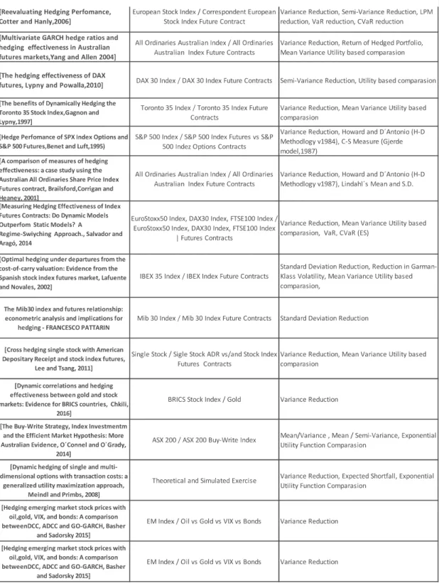
Regarding the hedging objectives, several conceptual approaches have been taken in the literature. Nevertheless, the traditional risk reduction target has been the most common and relevant Johnson (1960) and Ederington (1979). On the other end, as it will be discussed along this dissertation, hedging effectiveness can and should also be analysed and both risk minimization and return maximization as it is not costless neither riskless. Therefore, welfare improvement objectives have been considered Lypny & Powalla (1998). The hedging objective choice, the effectiveness measure and effectiveness measure parameters chosen are important considerations regarding the conclusion on the most adequate hedging model and contract. Cotter & Hanly (2006) evaluate the performance of different future contracts hedging ratios models in hedging equity markets indexes from US, Europe and Asia and proved that some performance metrics as the case of VaR provides different conclusions about the best hedging strategy when compared with pure variance minimization criterion. Gagnon & Lypny (1997) examine the effectiveness of dynamic hedging strategies of Toronto 35 Index Fuctures under the Variance and Welfare Maximization criteria. and showed investors risk aversion and transaction costs
consideration influence on hedging performance and comparisons. Brailsford et al. (2001) studied hedging effectiveness of Australian All Ordinaries Index Future Contract strategies applying different measures and illustrated that different effectiveness measures as HBS (1987) or the Lindahl measure (1991) produce different ranks for hedging models. Demirer et al. (2005) studied the effectiveness of Taiwan Stock Index Future Contracts based on Variance, Gini and LPM criteria and presented different performances and optimal hedging ratios depending on Variance, LPM or Gini criteria.
Variance reduction measure is the simplest risk reduction measure of effectiveness. It compares the standard deviation (s.d.) of the hedged portfolio with standard deviation of unhedged portfolio. Variance Reduction Metric can then be computed as:
Eq. 1
A equal to 1 means the full risk reduction, which means 100% effectiveness; a equal to 0 means 0% of risk reduction or a 0% effectiveness.
Variance has been the standard measure of risk for financial assets. Consequently, it has been applied by practitioners and academics in hedging performance assessment. Erdington (1979), used risk reduction as main metric in the very beginning of hedging activities with Treasury Bill Futures. As main advantages, the easy calculation, the straightforward interpretation and its applicability not depending on the hedging technique used can be appointed. On the other hand, several weakness and limitations have been referred in literature. Cotter & Hanly (2016) and others point out the following shortcomings. First, this metric focus exclusively on risk reduction and totally disregards consequences in hedged portfolio returns. The appropriateness of this criterion depends on whether the mean of the hedging instrument returns (net of costs) are zero. If they are not, the effectiveness is not correctly assessed, as shown by Lypny & Powalla (2010) that empirically shown that mean future returns were not zero using DAX future contracts. Second, and by definition, variance weights in the same way both positive and negative variations from the mean. Consequently, the upside and downside return probabilities are put in the same level. This is not totally accurate and reasonable because most of the times hedgers are generally more apprehensive about downside risk and therefore more focused with the left tail of the distributions of rates
of returns1. The third weakness pointed out relates to the assumptions of the
distributions of returns. On a non-normal distribution, which is the vast majority of the case of financial assets,(excess Kurtosis and Skewness different from zero are generally
observed in asset prices returns) the first two moments are insufficient to accurately describe the statistical distribution and therefore to evaluate the effectiveness of the hedging, Bookstaber & Clarke (1985). Finally, investor risk preferences are not considered.
When addressing the second, third and fourth variance shortcomings mentioned in previous section 2.2, several downside risk constructs were developed. One of the first approaches to handle the downside risk was suggested by Fihsburn (1977) with the - . It can be described as risk-dominance model and only accounts for those deviations that fall below a pre-defined target. It represents a probability-weighted power function of the shortfall from a specific target return Demirer et al. (2005) and it is fully consistent with the Von Neumann-Morgenstern expected utility model, Fishburn (1977). It uses no parametric assumptions and no constraints are needed regarding the distribution of returns, in particular the assumption of normality, Shadwick & Keating (2002). This is rather important for hedging performance measurement as it can provide tail probabilities of returns that follow non-normal distributions. The formulation for n-degree Lower Partial Moment computation are as follows:
Eq. 2
Where n represents the degree of LPM, represents the target return/thresholds, F(R) is the cumulative distribution of portfolio return. As we work with discrete return observations, the above computations can be simplified as:
Eq. 3
1Roy (1952)
With m standing for the number of discrete return observations, representing the rate of return of portfolio i at time t. The parameter n, the level of the LPM, is representative of investor fear and greed levels, and it is the result of the weight the model attaches to negative deviations from target return. The highest the parameter n, the greediest the investor and the highest level of investor risk aversion, Fishburn (1977).
Several values can be used for , such as the mean return, the risk-free rate, or zero if the investors main concern is avoiding negative returns. As it can be easily shown, the semi-variance is a special case of LMP, where level n = 2 and equal to the mean of the distribution. The use of downside risk measures like the lower partial moment has traditionally been justified as it is able to handle skewness. One very useful feature of partial moments is that they allow for different targets paired with different risk aversion degrees. Different values of n can approximate a wide variety of attitudes towards the risk of falling below a target return, Fihsburn (1977). Therefore, the model is highly configurable to multiple constraints and does not require any distributional assumptions, Viole & Nawrocki (2016). With respect to the Hedging Effectiveness Measure based on LPM risk metric, is proposed as follows:
Eq. 4
The following group of effectiveness measures include the popular tail-based Value-at-Risk (VaR) and its amended version, the Conditional Value at Value-at-Risk / Expected Shortfall (CVaR/ES). A popular intuitive definition for VaR, Jorion (2002), is that it summarizes the worst loss over a target horizon that will not be exceeded with a given level of confidence. Its use has been increasing as a measure of risk within financial institutions regulatory requirements and internal risk-management models, (2015).
Eq. 5 0 < n < 1 - risk seeking investor risky option dominates the sure-thing
n = 1 - risk neutral investor - indifference between risky option and sure-thing n > 1 - risk adverse investor sure-thing dominates the risky option
In a formal way, VaR describes the quantile of the projected distribution of gains and losses over the target horizon. In the context of the present work, VaR at confidence
level q will be given by the smallest number l that the probability that the loss L is higher than l, is smaller or equal than (1-q). It is derived from probability distributions but in our context, it will be empirically computed (Empiric VaR), using experimental distribution, by the sample quantiles of unhedged and hedged portfolios returns.
Eq. 6
Other methods not applied here include the parametric approximation and simulation. Empiric VaR ve the main relevant shortcomings of parametric VaR such as lack of subadditivity, normality requirements and need for appropriate adjustments such as Cornish-Fisher2 updated VaR version which includes the third and four
moments of the distribution. However, VaR results are quite sensitive and dependent on parameters, data, assumptions and methodology, Beder (1995), namely in the present case depend on q (the confidence level) which can lead to conflicting results. Aditionaly we have the fact that VaR can have many local extremes. On the other hand, VaR does not measure or inform about the losses exceeding VaR itself. In other words, VaR has no information content when the maximum VaR loss is exceeded. The magnitude and shape of the loss distribution is of importance in order to evaluate performance and hedging effectiveness. To address this specific VaR shortcoming, an additional metric was introduced accessing how deep is the loss in the case the maximum VaR loss is exceeded the CvaR (Conditional VaR) or ES (Expected Shortfall), Artzner et al. (1999).
Eq. 7
The at the q level can be formally interpreted as the expected loss on the portfolio (L), assuming is exceeded. It intuitively represents the Expected Loss (L) in the worst q % of the cases, Acerbi & Tasche (2002). Similar to VaR, can be computed either empirically or by parametric method using distribution parameters and upgraded with Cornish-Fischer adjustments mentioned above. We apply the empirical form only on order to overcome the early specified problems of the parametric VaR.
2Cornish-Fisher VaR includes the third and fourth moment of the distribution and consequently incorporates the advantage to evaluate non normal distributions of returns.
Eq. 8
Since hedging instruments returns are not martingales (expected mean returns are not zero in the vast majority of the cases), exclusive risk-minimization criteria and measures fail to capture the full risk-return trade-off that is inherent to any hedge, whether being static or dynamic and independently of the hedging instrument chosen,
tonio (1984). Acknowledging this basic approach, resulted to consider that return performance was not 100% adequate. Hence, several authors have studied hedging performance within a risk-return framework when future contracts are applied: Anderson & Danthine (1980 and 1981), Dale & Charles (1981). One of the most popular risk-return hedging effectiveness measure is HBS Hedging Benefit per Unit of Risk. HBS
applied to future contracts hedging and presented as a closed-form solution that could be used in a practical manner:
Eq. 9
Where is the risk to excess return relative of futures versus the spot position (risk-return relative) and representing the spot-futures correlation coefficient. It incorporates both, the minimization of risk and the maximization of excess return. This original HBS metric shown in Eq.9 was later analysed and tested by Chang & Shanker (1987). However, they have pointed out that this measure produces incongruent and ambiguous parameters (infinite optimal hedging positions) and results. Those shortcomings were con
an upgraded model that was considered quite superior:
In equation 10, represents the return of the unhedged portfolio (spot returns), the return of the hedged portfolio; the risk-free rate, the standard deviation of unhedged portfolio returns and the standard deviation of hedged portfolio returns. From algebraic arrangements can be notice that in essence, the updated version of HBS represents the relation between the Sharpe Ratios of hedged and unhedged portfolios.
As it was previously referred, the aim of maximization of return by unit risk is the base of HBS measure. Moreover, transaction costs and other direct and indirect costs can be incorporated by using net returns of the hedged portfolio. A positive HBS (HBS> 0) means that hedging is a performant activity, while if HBS < 0 suggests hedging as a non-performant activity and suggests that benefits are not covering costs (transaction and other direct and indirect costs considered).
HBS was built within the variance theory and takes into consideration mean-variance investor preferences. Despite of this, it became one of the most referenced metrics regarding future hedging effectiveness. However, HBS (1984 and 1987) versions have been criticised by several other authors such as Kuo & Chen (1995) and Satyanaraya (1998), mainly regarding practical simplifications and also focusing priori assumptions about risk-return between spot and futures. Also, Lindahl (1991) identifies several drawdowns, namely that HBS focus on hedged returns vs spot returns, rather than hedged return vs equilibrium return. Lindahl (1991) argues that equilibrium return should be risk-free rate in a fully hedged portfolio, under perfect equilibrium conditions and not considering transaction costs. Lindahl (1991) proposes an alternative measure. However, as it is composed of two parameters and it creates difficulties regarding its empirical application on evaluating hedging strategies, when comparing and ranking different hedging methods. We will use HBS, presented by Howard &
(1987) as an alternative effectiveness measure.
Eq.10
Although risk, using variance as proxy, and risk-return measures are widely applied to assess and to compare hedging effectiveness of different instruments and hedging strategies, a main shortcoming is raised: they do not consider investor
the risk-return trade-off, namely on the
drawback, hedging effectiveness of several hedging ratios for future contracts were measured applying an utility based approach by Ceccehetii et al. (1988), Gagnon et al. (1998), Yang & Allen (2004), Lypny & Powalla (2010), Kroner & Sultan (1991). The referred improvement of utility-based measures is furthermore motivated by the increasing use of dynamic hedging strategies and consequently higher transactions costs. Assuming a quadratic utility function built within the mean-variance framework, the Average Utility U is presented as an ex-post measure for a portfolio and can be
defined as, Kroner & Sultan (1991), Gagnon & Lypny (1997), Alizadeh & Nomikos (2004):
Eq. 11
Where is the portfolio average Utility, portfolio mean return, the variance of the portfolio rates of return and t tolerance parameter aversion. Hence, the risk profile of the investor can be adjusted and therefore investor preferences can be taking into account. When applying this performance metric, we are able to measure the utility gains or losses and, consequently, the economic benefits of different hedging strategies including the unhedged alternative. A hedging strategy is economically superior to other if it produces higher utility after transaction and indirect costs to be taken into consideration Gagnon et al. (1998). A strategy will be considered superior if its utility gains exceed the extra costs, when comparing the full or partial hedge strategies with the unhedged strategy. Another example is the comparison of static strategies with dynamic and more expensive strategies Kroner & Sultan (1993). Maximizing Utility within the hedging context, can be analysed on the two terms of the equation Gagnon et al. (1997). The second term translates the pure-hedging and risk minimizing position weighted by risk aversion profile. The first term can be interpreted as taking into account speculative demand of hedging instrument reflected into hedged position return, Lypny & Powalla (2010). Economic benefits of several models and different hedging strategies will be accessed comparing their utility gains.
Eq. 12
In the current study, the performance of the unhedged portfolio will be used as benchmark against all hedging strategies that will be evaluated using different effectiveness measures.
The main reasons for trading futures contracts are hedging, speculation, arbitrage operations, risk sharing and price discovery, Johnson (1960) and Silber (1985). In a
particular way, stock index futures can offer opportunities to split and capture the market and non-market components of risk and return that will then be used by money managers, investment banks and hedge funds. A good illustration is the use of stock index futures in program trading and index arbitrage, exploring price correlations between spot and futures prices. On the other way, hedgers use futures contracts as a tool to avoid or to minimize risks associated with price changes in cash/spot markets. The exercise of hedging depends critically on the estimation of the hedge ratio. In its simplest definition the hedge ratio is the number of futures contracts needed to minimize the exposure of a unit worth of a spot market position. Therefore, an investor holding a spot long position would short units of futures contracts - is then defined as the hedge ratio. When looking for the optimal ratio that minimizes the risk and optimal hedge ratio (OHR).
The earlier suggestions in the OHR literature may be found in Johnson (1960) and Ederington (1979). Early times research on OHR computation in late 1970s and early 1980s started to apply a standard and traditional regression analysis, assuming a time invariant OHR and normally distributed asset prices returns, Ederington (1979). However, most research that has been carried out recently, show that most asset returns are not normally distributed, i.e. empirical distributions show high skewness and excess kurtosis and, moreover, changing with the times. Consequently, several authors have been evaluating the performance and presenting alternative models to time invariant OHR proposed by Ederington: Park & Switzer (1995) for stock-index markets; Kroner & Sultan (1991 and1993) for foreign currency futures markets; Baillie & Miers (1991); Garcia et al. (1995) for commodity futures and Gagnon & Lipny, (1995) for interest rate futures. The main contributions of these authors are related with time variant conditional hedge ratios. Despite the fact time variant hedge ratio concept is generally appealing, the market application and estimation of this parameter involves an effective modelling of correlations between the spot and the futures prices/returns which can lead to further assumptions and shortcomings, subjects to be addressed in this study. In order to control the influence that different OHR computation methods could bring to our study we apply several of them from the ones that are presented in the literature. These time invariant conventional Ordinary Least Squares (OLS), the dynamic time variant rolling window OLS, the EWMA (dynamic and time variant) and the GARCH model (dynamic and time variant).
The naive hedging strategy is the simplest OHR model: Brooks & Chong (2001) and Cotter & Hanly (2006). This traditional strategy stresses the potential of futures contracts to hedge market risk and involves the hedger to sell a futures contract position that is equal in magnitude to the spot long position. Consequently, in this strategy it is assumed that OHR = -1. Therefore, if spot and future prices both changed by the same
amount, the investor net position would be unchanged. That would be the case of a perfect hedge. However, in real markets it is very unlikely to observe such a perfect hedge, with a unitary and time invariant correlation between spot and future prices. Consequently, the hedge ratio that minimizes the variance of the hedged portfolio should differ from -1, Kenourgios et al. (2008).
Eq. 13
In most of the times a perfect hedge is not achievable. Even in the case of a long portfolio position that exactly matches the composition of the f s contract used to hedge. On top of this it is also unlikely that the hedging horizon also matches, precisely, the maturity of the futures contract. In the most common situation, investors are exposed to basis risks caused by changing differences between spot and futures returns. In the literature addressing this subject one prevalent approach was developed by Johnson (1960) , by Stein (1961) and then applied by Ederington (1979) . It is based on modern portfolio theory and applies risk and return definitions in terms of the mean-variance framework. The objective and main goal was defined as risk minimization. In this model, risk is defined as the variance of returns on an two-asset hedged portfolio. Assuming investors face a mean-variance expected utility function, the optimal number of future contracts corresponds to the one that maximizes the expected utility computed with investors risk aversion parameter , Kroner & Sultan (1993).
Eq. 14 Where represents futures expected price changes, the unconditional covariance between spot and futures price changes and the unconditional variance of future price changes. Assuming that futures prices follow a martingale,
then, , where represents Futures contract price at time t, the variance minimizing hedge ratio results as follows:
Eq. 15
A simple estimator of Eq.16, which represents the minimum variance hedging ratio and that is commonly and widely used by practitioners, is the slope of the OLS estimated on the changes of the logarithm of spot prices against the changes of the logarithm of futures prices, Jonhson (1960) and Ederington (1979). It can be mathematically described as below:
Eq. 16 Where and represent the changes in the logarithm of spot and future prices,
, , and are respectively the intercept, the slope, the error and the error variance of an OLS linear regression estimation. The linear regression is estimated from all sample data available before the hedging start. Jonhson (1960) and Ederington (1979) proposal has been criticised by several authors: Park & Bera (1987) show the misspecifications of OLS for direct and cross-hedging of interest rate risk and Herbst et al. (1989) showed that within currencies hedging with future contracts OLS regression can yield biased and suboptimal results when normality, constant variance (homoscedasticity) and uncorrelated error terms assumptions were not satisfied, as it is the case of future rates of foreign currencies. Taking advantage of significant advances in time series analysis and computational econometrics, they have proved that minimum variance, constant OLS hedge ratio suffers from serial correlation and ignores the heteroscedasticity that is often found in cash and future price returns series. Consequently, it has been widely argued about the inefficiency and non-optimum OHR estimates obtained by simple and time invariant OLS regression.
Despite its simplicity and low transaction costs, the conventional time invariant OLS hedging model cannot and does not update the information known at the time of hedging decision. This leads to an inefficient estimations of OHR, in particular when out-of-sample forecasting and estimations are to be made, Kenourgios et al. (2008). This shortcoming may be overcame by applying the variant rolling window method which involves the use of a rolling-window estimator to the variance-covariance matrix. OHR are sequentially re-estimated with the dynamic hedging roll-over where the most recent data observations replaces the oldest one, keeping the sample size number constant. The OLS estimation is rolling over as we hedge out-of-sample, therefore incorporating the latest information and discarding the most out-dated information, Cotter & Hanly (2006). The main advantage of this model is that it takes into consideration time varying return distributions used to estimate the OHR. On the other hand, as other models that implement time varying hedging ratios, transaction costs are consequently increased.
Eq. 17
represents the slope of the OLS linear regression represented by Eq.17 and estimated with a rolling-window data sample.
The Exponentially Weighted Moving Average (EWMA) forecasting method was popularized by RiskMetricsTM. RiskMetricsTM, J.P.Morgan & Reuters (1996), was one of the first high popular risk-measurement software applications. RiskMetricsTM was based on VaR the Value at Risk concept. The popular application forecasted variance and covariance estimators by applying an EWMA model. It is similar to the OLS ratio but uses an exponentially weighted average in order to estimate ,
conditional variance of future price changesand ,conditional covariance between spot and futures price changes.The one-day forecast equations, assuming the mean value of daily returns is zero3 4as in RiskMetricsTM, J.P.Morgan & Reuters (1996):
With representing the decay factor. This parameter introduces the weights that are allocated to the last observations and the amount of past data taken into account when estimating volatility. The parameter weight declines exponentially over time. In this empirical study the decay factor was set equal to 0.94 ( ) as the optimal decay factor according the following criterion: minimizing the 1 day ahead forecasted variance root mean square error, RiskMetricsTM (1996). EWMA has two main advantages, Brooks & Chong (1985), over simple-historical models as described below. The volatility is more influenced by the most recent events than by the past events; and the effect on volatility of a single observation declines exponentially. This is particularly significant in the case of strong shifts on prices. Keeping them in the estimating sample causes erroneous estimations. Therefore, letting them to fall out of the sample if they are kept in the sample would tend to increase the accuracy of the estimation, since the model allows for the come back to normal values. Consequently, the time varying estimate of the hedge ratio can be given by
3Ignoring expected return is unlikely to cause a relevant bias in the volatility estimate. (RiskMetricsTM, 1996),(Jorion,1995).
4 Implies that standard deviation estimates are centred around zero and deviations of returns are centred around zero (RiskMetricsTM, 1996)
Eq.15
The previous methods apply a simple (static or rolling) OLS regressions or EWMA models for optimum hedge ratio estimations. Nevertheless, the vast majority of prior highlighted academic and practice studies state that a simple regression model is not the appropriate model to estimate optimum hedge ratios due to the existence of correlation between OLS residuals. Additionally, it is assumed the common existence of heteroskedasticity in spot and future prices time series as showed by Herbs et al. (1993). As an example, Bell & Krasker (1986) argue that, if expected futures price returns depend on the information set available at the hedging decision moment, hence the simple OLS method that involves only unconditional moments and consequently unconditional hedge ratios, is not optimal. Therefore, for the purpose of estimating OHR, Myers & Thompson (1989) considered that the covariance between spot and futures price returns and the variance of futures price returns should be conditional on the time and depending on the information set at hedging decision studied when applied to storage hedging of corn, soybeans and wheat. As a result, the hedge ratio should be time variant and it should be adjusted based on available information. This in turn raises concerns about the effectiveness of OLS hedge ratios. To address the problem, several studies like in Myers et al., (1989), Kroner & Sultan (1993), Park & Switzer (1995), Gagnon & Lypny (1995), Lypny & Powalla (1998), Yang & Allen (2005) have applied Generalized Autoregressive Conditional Heteroskedasticity (GARCH) model to estimate varying variances and covariances and consequently resulting in time-varying hedge ratios. The main rationale behind GARCH models is volatility clustering, that is characteristic of financial assets (in both spot and futures prices returns, Mandelbrot (1963). Consequently, this result implies that the second moment of spot and future assets returns should be time dependent and continuously updated with available information set. An useful generalization of previous ARCH/GARCH models introduced by Bollerslev (1986) is the GARCH (p,q) that defines the volatility as a function of unexpected information shocks to the market.
The generic conditional mean, conditional variances and covariances equations of the simplest (1,1) version of GARCH class models are as follows:
Where and are the spot and futures prices log returns and and stand for the spot and the futures price returns prediction errors (residuals), i.e., innovations, also known as shocks at time .
Eq. 20
Where symbolizes the updated information set at time and the conditional variances. The referred model for the conditional covariances matrix can be written as:
Where compose the variance-covariance matrix. They are conditional variances and covariances to be forecasted, resulting in time varying conditional hedge ratios. The error terms represent innovations or shocks and correspond to a (2x1) vector. Model parameters and operators can be listed as follows:
is the intercept (3 x 1) vector parameter, and are (3 x 3) parameters matrices. Vech is the half-vectorization operator that operates a linear transformation that converts the lower triangular part of a symmetrical matrix into a column vector. The model parameters shown above, the Vector are estimated as the ones that maximize the log-likelihood function for sample observations. Assuming the conditional distributions of innovations / shocks are normally distributed, the log-likelihood function for a sample of T observations of spot and futures prices is as follows by Myers (1991) and Bollerslev et al. (1988):
One of the GARCH versions is the constant-conditional-correlation GARCH (CCC-GARCH) as in Bollerslev (1990). Assuming that the conditional means of spot and futures price returns follow an Autoregressive Process as follows:
Eq. 21
Then it is feasible that a CCC-GARCH (1,1) may apply with a constant rolling 100 days conditional correlation between spot and future returns:
According to Bollerslev (1990), the maximum likelihood estimate of correlation matrix is equal to the sample correlation matrix. As the sample correlation matrix is positive semidefinite, parameters are estimated subject to conditional variances being positive, which simplifies the computation and operation of the model on a rolling-window framework. After one-step ahead covariance matrix forecast, the dynamic optimal time varying hedge ratios for the correspondent time period can be directly computed according to:
Eq. 15
As an example, this method was used to estimate time varying OHR for currency futures hedging by Kroner & Sultan (1993), for stock index futures by Park & Switzer (1995) and for currency futures hedging by Lien et al. (2002).
The data set compromises closing prices daily data of stock indexes of Portugal (PSI20), Greece (ASE), Cyprus (CYSMMAPA), Belgium (BEL20) and Austria (ATX) and future contracts daily data written on Eurostoxx 50, DAX 30 and CAC40. The formers are representative of the smallest and the less liquid stock indices of euro-area region. The represent the most liquid future contracts from the same region. Using daily Data allow us to take empirical conclusions, simulating portfolio managers who adjust their portfolio daily. Additionally, several studies presented by Lien et al. ( 2002) have concluded that hedging performance turns to be higher over short periods of time. Nevertheless, it is expected that portfolio managers do not rebalance their holdings every day. Either mathematically or intuitively, they tend to rebalance their
Eq. 23
portfolios when increased expected utility from adjustment is high enough to cover transaction costs, Kroner & Sultan (1991 and 1993). Therefore, numerous studies and prior research have used weekly data. In the former case, and for weekly portfolio rebalance Wednesday closing prices were used to mitigate the beginning and the end of the week effects following the conclusions of Berument & Kiymaz (2003) that showed the presence of week effect on stock market volatility (S&P500). When a
was used instead.
Daily returns are computed as the differences of natural logarithms of consecutive daily that at all rollover date return computation is taken over the same contract.
Index and futures contracts data were obtained from Bloomberg. The sample period range is from 2011-01-03 to 2018-04-04. Market holidays were excluded. Given the fact that future contracts have an expiration (maturity) date, for each future contract a single continuous time series of futures prices had to be build. Several authors propose series, Ma et al. (1992), Carchano & Pardo (2008)5. We estimated a time series based on spot futures contracts
for liquidity reasons. To avoid the expiration effects and thin trading, futures positions are assumed to be rolled-over to the nearest spot futures contract on the day the spot futures contract expires. As example, the rollover of the March contract that expired on the 31th March was rolled over on the 31th of March to the spot futures contract. To
compute the continuous time series price change (for the rate of return calculation) for 31thMarch, we used the 30thand 31thof March prices of the same contract.
The sample was divided into two subsamples:
a) Sample 1 that is composed by 1,282 daily observations collected from 2011-01-03 to 2015-12-31. This subsample was used to calibrate the hedging models (main propose) and to evaluate an hypothetic in-sample hedging performance as also historical performance.
b) Sample 2 that is composed by 577 daily observations collected from 2016-01-04 to 2018-04-04. This subsample was used to perform and measure out-of-sample hedging performance : investors are far more concerned with how well they will perform in real future using each one of hedging strategies. Therefore, out-of-sample performance is a more realistic way to evaluate and compare hedging effectiveness.
The full sample descriptive statistics and several diagnostic checks for both spot and futures price returns distributions are summarized in Table II, showing the results for
5Carchano and Pardo showed that there are not relevant differences between the resulting continuous series and that therefore the least complex method can and should be used.
the mean, the standard deviation, the variance, the skewness6, the excess kurtosis7, the
Jarque-Bera Test8, the augmented Dickey-Fuller (ADF)9and LM10tests statistics.
Table II : Descriptive Statistics of Stock Index Spot and Futures Log Returns
The full sample spot stock indexes distributions are similar in terms of mean values, that is, they are approximately zero. The ASE and CYSMMAPA stock indexes present the most volatile distributions in terms of daily log returns. The full sample of futures price returns distributions are similar in terms of means and standard deviations. The full sample time series distribution exhibits conditional heteroscedasticity which is relevant for the validity of the GARCH models, and it will be taken into consideration in time variant conditional hedge ratios. On the other hand, ADF test statistic supports the stationarity of the full time series, allowing to reject the possibility of spurious
6Skewness equals to zero in Gaussian Normal Distribution.
7Excess kurtosis represents the departure from the normal distribution skewness parameter of 3.
8The null hypothesis of the Jarque-Bera normality test is a joint hypothesis of the skewness being zero and the excess kurtosis being zero. With a p-value > q, one would conclude that the data are consistent with having skewness and excess kurtosis zero at q% confidence level.
9The null hypothesis of the Augmented Dickey-Fuller represents the existence of a unit root in the sample indication of non-stationarity. With a p-value < q, one would conclude the rejection of the null hypothesis at q% confidence level.
10Lagrange multiplier (LM) test for the null hypothesis of no conditional heteroskedasticity against an ARCH model. With a p-value < q, one would conclude the rejection of the null hypothesis at q% confidence level and therefore the presence of conditional heteroskedasticity in the sample.
regression results for the hedge ratio regressions methods. The full detailed statics tests are presented in Appendix D.
The aim of this research is to test whether liquid futures contracts are good instruments to hedge local non-directly related national index portfolios of smaller countries. In order to do so, we selected several hedging effectiveness measures (HEM) as found in the literature, to assess the use of several optimal hedge rations (OHR). The HEM are the ones previously described and are numbered from 1 to 6 (HEM1to HEM6). They
are used as criteria to test the goodness of using cross hedging in illiquid national portfolio management with futures contracts. For each index, we used 5 different hedging ratio computation methods in order to control for the methodology dependence.
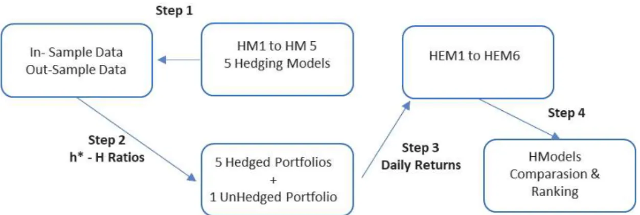
For each national stock index both in-sample and out-sample, the steps to proceed are as follows and as illustrated in figure 1: i) Hedging Ratios h* are computed according the hedging models described above (HM1 to HM5). ii) The five different resulting
Hedged Portfolios log returns were then computed (from the application of the previous calculated h*). iii) Daily log returns were then computed for both the Unhedged and Hedged Portfolios. iv) Each Hedged Portfolio was then evaluated according to each of the 6 different Hedging Effectiveness Measures (HEM). Finally, the unhedged portfolio, and the different Hedged Portfolios were subsequently ranked according HEM criteria.
Ratios and EWMA Ratios computation are simple applications of theoretic formulations explained in chapter 3.
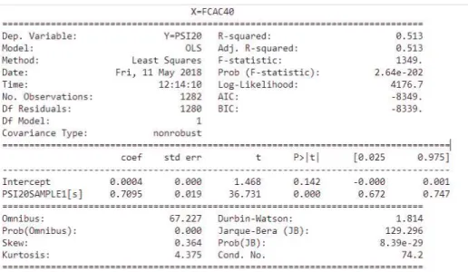
As example of In-Sample OLS regression output for the PSI20 as the portfolio to be hedged and the CAC40 futures contract as the derivative instrument to be used for hedging (Y= PSI20, X=FCAC40) is shown in figure 2 where R-Squared and Adjusted R_Squared quantify the explanatory power of OLS model. Positive and non-zero OLS repressors representing the slope, at 5% Confidence level are used as h* estimators, according to the literature explained in chapter 3.
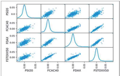
We can conclude, from both figure 3 plot and Appendix E Figures 8 - 11 plot (Appendix E presents scatterpltot matrices for the remaining analysed Stock Indexes) that pair-wise correlations between the peripheral PSI20, ASE and CYSMMAPA stock indexes and the futures contracts shown significant differences in terms of
linearity when compared with Central Europe BEL20 Index equivalent pair-wise correlations
The In-Sample CCC-GARCH at 95% confidence level results are presented with detail in Appendix C. Results show that in the majority of the cases GARCH models coefficients are positive and statically significant at 5% confidence level. The parameter sum in each equation is close to unity which suggests the persistence of ARCH effects in the data sample. Therefore, the available information is relevant for conditional variances and covariances all horizons forecasting, Yang & Allen ( 2005).
The CCC-GARCH model is re-estimated each week during the out-of-sample period and out-of-sample hedge ratios are generated by one-step ahead forecasts of the time-varying variance-covariance taking into consideration all information available at hedging time.
Table III : GARCH Models Specifications and Orders Figure 3: PSI20, FCAC40, FDAX, FSTOXX50 Scatterplot Matrix
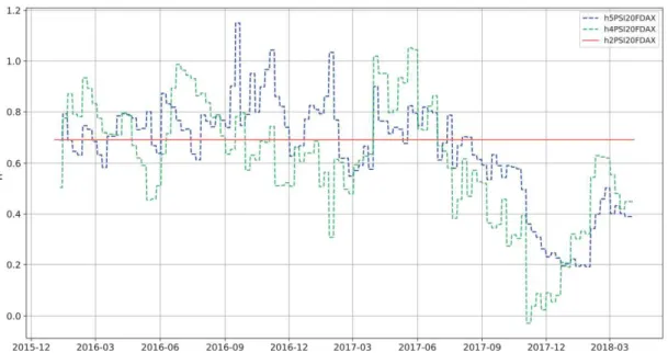
The Optimal Hedge Ratios at 95% confidence are presented by the following acronyms: h,[model n
instrument]. The Graph from Figure 4 compares time-variant with static OHR. We can conclude that time-variant hedging ratios lead to highly frequent rebalances on hedging strategies with very different compositions when compared to constant hedging strategies. Only an analysis of risk/return efficiency like the one presented and which conclusions are described in chapter 5.3 allow us to compare and quantify the real efficiency
.
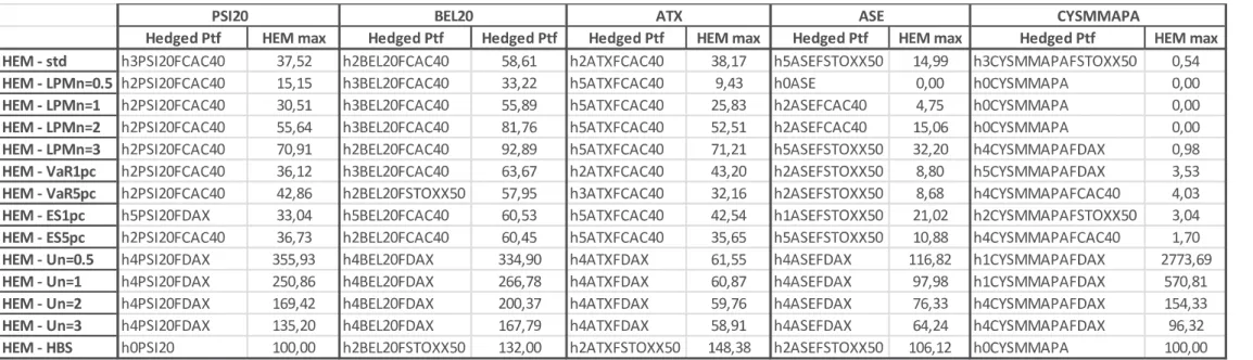
The empiric results for PSI20 hedging effectiveness measures for Out-Sample back testing and for each OHR are presented in Table IV. Both In-Sample and Out-Sample empirical results for all the other four stock indexes are presented in Appendix B. Although hedging strategies in-sample performance can give an indicator of their historical performance, investors are far more concerned with how well they will perform in real future using each one of hedging strategies. Therefore, out-of-sample performance is a more realistic way to evaluate and compare hedging effectiveness.
HEM1 Variance Reduction: All hedging models result in a variance reduction. For the out-sample results, the best outcome was a reduction of 37.52% when compared to unhedged portfolio. This was achieved applying the rolling OLS time varying hedging ratios with the CAC40 futures contracts. The less effective corresponds to a hedging
st ing ratio.
Therefore, it can be concluded that in this particular case time varying hedging ratios outperform the constant ones. Moreover, less complex time varying models as rolling OLS and EWMA outperform more complex time varying conditional variance models as the GARCH type models.
HEM2 Lower Partial Moments: As expected, the higher the level of investors risk aversion, the higher the downside risk reduction and therefore the lower the LPM. On the other hand, the most efficient future contract to use is the one written on the CAC40 index. The static OLS ratio model outperformed all the time varying and conditional hedging ratios models.
HEM3 VaR: Taking into consideration the tail based downside risk reduction, the hedging model using CAC40 futures contracts is the most effective and a reduction between 36,12% and 42,86% was achieved applying the static OLS model for hedging ratio computation. Hence, the static and less complex models outperform the more complex and sophisticated time varying models.
HEM4 ES: According to the extreme tail based downside risk measure we have two contradictory results: the GARCH model ratios with DAX futures contracts was the most effective at ES 1% but the static OLS with CAC40 futures showed the highest ES 5% reduction.
HEM5 Utility Increase: Taking into consideration an Utility/Economic Benefit measure the most effective Hedging Strategy was found by applying the EWMA model to DAX futures contracts with an increment between 135,20% and 355,93%. The
under- the STOXX50
futures.
HEM6 HBS: According the HBS measure, that takes into account both return and standard variation, all studied strategies fail to increase the HBS when compared to unhedged PSI20 portfolio. The worst performer was the EWMA model using the DAX futures. On the other hand, the static OLS model with the STOXX50 futures showed the highest HBS.
In table IX we can analyse a wider out-sample (ex-ante) scenario where for each stock Index and each HEM, the pair strategy/models presenting the best performances are highlighted.
For the PSI20 the best performant futures contracts were those written on the CAC40 and on the DAX. Static OLS and the EWMA are in general, the hedging models that show, respectively, the highest risk reduction and maximum utility maximization. No hedging strategy is effective when measured with HBS. Additionally, taking into account transaction costs would result in even lower values for effectiveness measures as HBS.
The BEL20 showed the best results among all the 5 local indexes that were tested in the hedging simulation. In terms of risk reduction performance (HEM1 to HEM4) the
OLS hedging models on the CAC40 futures contract can achieve for example a VaR 1% reduction of 63,67%. The highest level of Utility maximization and for all risk aversion levels are achieved with EWMA hedging models with DAX futures contracts (HEM5 Un=0.5 =334,90%). On the other hand, the maximum HBS measure, which considers risk/return yields 132% when applying static OLS hedging model.
ATX: a standard risk reduction of 38.17% is achieved with static OLS method applied to CAC40 Futures Contracts. The other risk reduction measures that present the highest levels of reduction correspond to GARCH hedging ratios models with CAC40 Future Contracts (HEM4(ES 1% reduction of 42.54%). Utility maximization is achieved with
EWMA models applied to hedged portfolios including DAX futures contracts (334,90% increase for the lowest level of risk aversion).
ASE: non-relevant risk reductions are achieved. GARCH hedging model with STOXX50 Futures yields a 32.20% reduction on HEM3 - LPM for the less risk averse investor. VaR and ES achieved reductions are non-relevant. Utility highest increases (116,82%) are achieved with EWMA model with DAX Future Contracts. All other risk measure reductions are not relevant in terms of hedging strategies success
CYSMMAPA: presents the least performant hedged portfolios. Risk Reduction Measures present approximately null results independently of the hedging model/instrument applied. Utility benefits results can be considered non-relevant in due to almost inexistent risk reduction. HBS measure confirms the non-satisfactory results of hedging on the risk/return framework This is consistent with lower correlation between the CYSMMAPA spot and the futures contracts in use as compared with the other markets as it can be observed in Figure 7 - Appendix E.
In average (considering HEM1 to HEM4), as we can observe in Table IV, (except of the case CYSMMAPA), positive hedging performance results were obtained: from the lowest 9.47% (ASE) to the highest 60.82% (BEL20).
Table IV: Hedging Effectiveness Empirical Results (%) Simple Average considering HEM1 to HEM4
HEM1| HEM2 | HEM3 | HEM4 | HEM5 | HEM6 | Table V : PSI20 Hedging Effectiveness Out-of-Sample Empirical Results (%)
This additional analysis presented in Tables VI and VII was performed with the main objective of measuring the out-of-sample (ex-ante) effectiveness of the different hedging models for PSI20 portfolio during two of the most volatile weeks of the last 5 years in financial markets - 2017 Presi In average (Table VII) we observed that hedging performance during this short high volatile period is higher than the one measured during long-term market periods: 54,32% two weeks period and 77,78% for USA Elections two weeks period against 37.64% corresponding to long term hedging period (see Table IV). Taking into consideration the results obtained for each Hedging
Table VII : PSI20 Average Hedging Effectiveness in USA 2017 Elections HEM max corresponds to the hedging model with maximum effectiveness.
Table VI: PSI20
Effectiveness Measure: HEM1: OLS hedging models with STOXX50 and CAC40
Futures yields the highest performance achieving a 91,81% risk measure reduction during Brexit Referendum period. HEM2
example a relevant 98,71% reduction of LPMn=2 in USA Presidential Election week
while Rolling OLS with CAC40 futures yields 99,30%. HEM3: high reduction of tail
risk measures between 81,79% VaR1%
contracts in USA election case. On the other hand 93,06% reduction in VaR5% is
HEM4: a disparity of results is
yields 88.95 % increase within USA Election week, however no increase is found in event. HEM5: relevant performance is measured
model with DAX Futures (153,11% - USA election) and using rolling OLS model to CAC40 Futures contracts.
This study analyses and measures the goodness of using cross hedging with the most liquid future contracts. They were applied several and the most used econometric models applying futures contracts and they were accessed under different criteria. Simple Standard Risk Reduction, Lower Partial Moments, Tail and Extreme Risk, Economic Benefit and HBS metrics are applied to the empirical case of cross-hedging European non-main stock indexes. The most relevant out-of-sample empirical results suggest that in general we have positive results from cross hedging and that the choice of the optimal hedging model and optimal future contracts to apply depends on the hedging effectiveness measure to be maximized. The choice of the hedging effectiveness measure to be applied should depend on main investing targets and concerns. Therefore, each investor should previously define its main and most relevant hedging objectives. Nevertheless, the majority of the empirical research results indicates the following: it is possible, and it results positive returns to cross-hedge the most illiquid European stock indexes with the most liquid European future contracts. Secondly and as expected, cross-hedging performance showed poorer results when compared to direct hedging performance. Direct hedging strategies Performance on the ASE index can be found in Kavussanos & Visvikis (2008). Thirdly the
OLS and EWMA econometric models generally outperform the more complex GARCH models. Similar results were found by Cotter & Hanly (2006). Fourthly, the most peripherical countries indexes (ASE and CYSMMAPA) have in average the poorest hedging effectiveness results. Lastly, the market jitters studied, namely the USA 2017 Election and the Brexit Referendum periods tested for the case of PSI20 indicate that in average short term hedging yields are better than long term hedges yields. Relevant tail risk reduction (HEM3) is .
On the other hand, we could have assumed that integration between economies could be other reasonable indicator to choose and to rank the cross-hedging instruments. The
weight of (Imports + Exports) in GDP ratio was used as ratio to test this assumption. As an example of the ratio between Portugal (PSI20) and Germany (DAX), it would be computed as ( Imports+ Exports)Portugal,Germany / GDPPortugal. From the average
results presented in table VII we cannot validate that assumption. Historical back-testing should be used instead, as it was performed during this study.
Four extensions of this study are suggested for future research: These are: to study the adequacy of each hedging performance measure to each investor risk profile, to consider transaction costs that can assume significant relevance in time varying ratios strategies performance, to apply Optimum Hedging Ratio models based on VaR or ES reduction criteria , and to allow for Conditionally Correlation, i.e. Correlation Spot-Futures to vary over time in an Generalized GARCH model.
Table VIII: Economical Integration Ratios
Germany France Germany France 5,77% 4,48% 5,69% 4,31% 3,08% 1,20% 2,88% 1,16% 26,95% 22,06% 26,12% 22,21% 29,10% 2,69% 28,61% 2,86% 5,80% 1,45% 2,51% 0,98% 2016 2015
.
AbulBasher, S. & Sadorskyc, P., 2016. Hedging emerging market stock prices with oil, gold, VIX, and bonds: A comparison between DCC, ADCC and GO-GARCH. s.l., Energy Economics 54, 235-247.
Acerbi, C. & Tasche, D., 2002. On the coherence of expected shortfall. s.l., Journal of Banking & Finance 26 (7), 1487-1503.
Alizadeh, A. & Nomikos, N., 2004. A Markov regime switching approach for hedging stock indices. s.l., The Journal of Futures Markets 24 (7), 649-674.
ANDERSON, R. W. & DANTHINE, J., 1980. Hedging and Joint Production: Theory and Illustrations. s.l., The Journal of Finance XXXV (5), 487-495.
Anderson, R. W. & Danthine, J.-P., 1981. Cross Hedging. s.l., Journal of Political Economy 89 (6), 1182-96.
Artzner, P., Delbaen, F., Eber, J.-M. & Heath, D., 1999. Coherent Measures of Risk. s.l., Mathematical Finance 9 (3), 203 228.
Baillie, R. T. & Myers, R. J., 1991. Bivariate garch estimation of the optimal commodity futures Hedge. s.l., Journal of Applied Economics 6 (2), 109-124.
Beder, T., 1995. VAR: Seductive but dangerous. s.l., Financial Analysts Journal 51 (5), 12-24 .
Bell, D. E. & Krasker, W. . S., 1986. Estimating Hedge Ratios. s.l., Financial Management 15 (2), 34-39.
Benet, B. A. & Luft, C. F., 1995. Hedge performance of SPX index options and S&P 500 futures. s.l., The Journal of Futures Markets 15 (6), 691-717.
Bessis, J., 2015. Risk Management in Banking.
Bollerslev, T., 1986. Generalized autoregressive conditional heteroskedasticit. s.l., Journal of Econometrics Volume 31 (3),307-327.
Bollerslev, T., 1990. Modelling the coherence in short-run nominal exchange rates: a multivariate generalized ARCH model. s.l., The review of economics and statistics 72 (3),498-505.
Bollerslev, T., Engle, R. F. F. & Wooldridge, J. M., 1998. A Capital Asset Pricing Model with Time Varying Covariance. s.l., Journal of Political Economy 96 (1), 116-131 .
Bookstaber, R. & Clarke, R., 1985. Problems in Evaluating the Perfomance of Portfolios with Options. s.l., Financial Analysts Journal, January-February, 48-64. Brailsford, T., Corrigan, K. & Heaney, R. A., 2001. A comparison of measures of hedging effectiveness: A case study using the Australian All Ordinaries Share Price Index Futures contract. s.l., Journal of Multinational Financial Management 11 (4-5), 465-481.
Brooks, C. & Chong, J., 2001.
Versus Statistical Forecasting Models. s.l., The Journal of Futures Markets 21 (11), 1043-1069.
Rolling Over Stock Index Futures Contracts. s.l., The Journal of Futures Markets 29 (7), 684-694.
Cecchetti , S. G., Cumby, R. E. & Figlewski, S., 1988. Estimation of Optimal Futures Hedge. s.l., The Review of Economics and Statistics 70 (4), 623-630.
Chang, J. S. K. & Shanker, L., 1987. A Risk-Return Measure of Hedging Effectiveness: A Comment. s.l., The Journal of Financial and Quantitative Analysis 22 (3), 373-376. Cheung, C. S., Kwan, C. C. Y. & Yip, P. C. Y., 1990. The Hedging effectiveness of Options and Futures: A Mean-Gini Approach. s.l., The Journal of Futures Markets 10 (1), 61-73.
Chkili, W., 2016. Dynamic correlations and hedging effectiveness between gold and stock markets: Evidence for BRICS countries. s.l., Research in International Business and Finance 38, 22-34.
Cornew, R. W., Town, D. E. & Crowson, L. D., 1984. Stable Distributions, Futures Prices, and the Measurement of Trading Performance. s.l., The journal of Futures Markets 4 (4), 531-557.
Cotter, J. & Hanly, J., 2006. Reevaluating Hedging Perfomance. s.l., The Journal of Futures Markets 26 (7), 677-702.
Dale, C., 1981. The hedging effectiveness of currency futures markets. s.l., The Journal of Futures Markets 1 (1), 77-88.
Darren, O. & Barry, O., 2014. The Buy-Write Strategy, Index Investment, and the Efficient Market Hypothesis: More Australian Evidence. s.l., Journal of Derivatives 22 (1),71-89..
Demirer, R., Lien, D. & Shaffer, D. R., 2005. Comparisons of short and long hedge performance: the case of Taiwan. s.l., Journal of Multinational Financial Management 15, 51-66.
Ederington, L. H., 1979. The Hedging Perfomance of the New Futures Market. s.l., The Journal of Finance XXXIV (1), 157-169.
Fishburn, P. C., 1977. Mean-Risk Analysis with Risk Associated with Below-Target Returns. s.l., The American Economic Review 67 (2), 116-126.
Gagnon, L. & Lypny, G., 1995. He
distributions. s.l., The Journal of Futures Markets 15 (7), 767-783.
Gagnon, L. & Lypny, G., 1997. The Benefits of Dynamically Hedging the Toronto 35 Stock Index. s.l., Canadian Journal of Administrative Sciences 14, 69-78.
Gagnon, L., Lypny, G. J. & McCurdy, T. H., 1998. Hedging foreign currency portfolios. s.l., Journal of Empirical Finance 5, 197-220.
Garcia , P., Roh , J.-S. & Leuthold, R. M., 1995. Simultaneously determined, time-varying hedge ratios in the soybean complex. s.l., Applied Economics 27 (12), 1127-1134.
Glasserman P, X. X., 2014. Robust risk measurement and model risk.. s.l., Quantitative Finance 14 (1), 29-58.
Helms, B. P. & Martell, T. F., 1985. An Examination of the Distribution of Futures Price Changes. s.l., The Journal of Fulure Markels 5 (2), 259-272.
Herbst, A. F., Kare , D. D. & Caples, S. C., 1989. Hedging effectiveness and minimum risk hedge ratios in the presence of autocorrelation: Foreign currency futures. s.l., The Journal of Futures Markets 9 (3), 185-197.
Herbst, A. F., Kare, D. & Marshall, J., 1993. A time varying, convergence adjusted, minimum risk futures hedge ratio. s.l., Advances in Futures and Options Research 6, 137-155.
Hodgson, A. & Okunev, J., 1992. An Allternative Approach for Determining Hedge Ratios for Futures Contracts. s.l., Journal of Business Finance & Accounting 19 (2), 211-220.
A Risk-Return Measure of Hedging Effectiveness. s.l., The Journal of Financial and Quantitative Analysis 19 (1), 101-112. Howard, C. T. & D'Antonio, L. J., 1987. A Risk-Return Measure of Hedging Effectiveness: A. s.l., Journal Of Financial and Quantitative Analisys 22 (3), 377-381. Jonhson, L. L., 1960. The Theory of Hedging and Speculation in Commodity Futures. s.l., The Review of Economic Studies 27 (3), 139-151.
Jorion, P., 2002. Financial Risk Manager Handbook. GARP ed. s.l.:s.n.
Kavussanos, M. G. & Visvikis, I. D., 2008. Hedging effectiveness of the Athens stock index. s.l., European Journal of Finance 14 (3), 243-270.
Kenourgios, D., Samitas,, A. & Drosos, P., 2008. Hedge ratio estimation and hedging effectiveness: the case of the S&P 500 stock index futures contract. s.l., International Journal of Risk Assessment and Management 9 (1-2) , 121-134.
Kiymaz, H. & Berument, H., 2003. The day of the week effect on stock market volatility and volume: International evidence. s.l., Review of Financial Economics 12 (4), 363-380.
Kroner, K. F. & Sultan, J., 1991. Time-Varying Distributions and Dynamic Hedging With Foreign Currency Futures. s.l., Journal of Financial and Quantitative Analysis 28 ( 4),535-551.
Kroner, K. F. & Sultan, J., 1993. Time-Varying Distributions and Dynamic Hedging with Foreign Currency Futures. s.l., Journal of Finance and Quantitative Analysis 28, 535-551.
Kuo , C. & Chen, K., 1995.