A Work Project, presented as part of the requirements for the Award of a Master’s
Degree in Economics from the NOVA School of Business and Economics.
How can Financial Integration impact the Monetary
Transmission Mechanism
Mariana Neto Pires
#25913
A PROJECT CARRIED ON THE MASTER’S IN ECONOMICS PROGRAM UNDER THE SUPERVISION OF:
Professor João B. Duarte
How can Financial Integration impact the Monetary
Transmission Mechanism
∗
Mariana Pires
†January 2020
Abstract
We investigate whether the integration level of the Euro Area’s financial system influences the transmission mechanism of monetary policy. We compute the impulse responses of inflation and output, while implementing local projections on panel data comprising each member state and subsamples. For a low-level of financial integration, the responses of inflation and output to a tightening monetary action are close to null. For a high-level of financial integration, the responses of inflation and output to the same shock become negative. These findings suggest that the fragmentation of the financial system may limit the European Central Bank’s monetary policy transmission.
JEL:E44, E52, F36 and F45
Keywords: Monetary Policy, Local Projection, Monetary Union, Financial Integration.
∗I thank João B. Duarte for providing outstanding supervision. I acknowledge the useful comments and suggestions
from Christian Osterhold, Marina Feliciano and Pedro Neves. I am thankful to my family and friends for their support. Even though my work has greatly benefited from feedback, I am solely responsible for any errors and omissions.
1
Introduction
The creation of the Economic and Monetary Union (EMU) was an event well anticipated by the markets, which triggered an increase in the financial integration across the countries, that would later be known as Euro Area member states. This is the desired evolution for the financial integration, given that the existence of a highly integrated financial system is key for the European Central Bank (ECB) mission of ensuring price stability. Indeed, by transferring the task of conducting the Euro Area monetary policy to the ECB, it is crucial for there to be a high-level of financial integration to guarantee that the effects of any policy decision are uniform across member states.
The continued increase of financial integration was interrupted by the subprime mortgage crisis in 2007. The reversion of this tendency became a matter of concern, specially for the ECB, that needed for there to be a well functioning monetary transmission mechanism to fulfill its role as stabilizing authority. This revealed to not be possible, as other ordeals would later rise, further fragmenting the financial system. As a result of the disruption of the monetary transmission mechanism associated with the financial fragmentation, the ECB was forced to resort to unconventional monetary policy measures with the announcement of the Outright Monetary Transactions (OMT) program and with the agreement to create the European Banking Union.
In this paper, we investigate whether the integration level of the Euro Area’s financial system influences the transmission mechanism of monetary policy. In order to investigate the proposed premise, we look at the impulse responses of inflation and output to a monetary shock, using local projections on panel data, under two different scenarios. Indeed, we compute nonlinear responses for a scenario in which there is a low-level of financial integration and a second scenario in which there is a high-level of financial integration. The initial analysis considers a panel data comprising monthly data for each one of the 19 member states of the Euro Area from March 2002 through December 2018. We proceed to conduct an analysis based on subsamples, with the aim of comparing the responses of the member states that during the process of financial fragmentation diverged greatly from the Euro Area average, in terms of long-term interest rate, with the responses of the remaining member states that during the same period followed closely the Euro Area average.
Following this procedure, we find that, in the presence of a low-level financial integration, the impulse responses of inflation and output to a tightening monetary policy are close to null. In contrast, when we consider that there is a high-level financial integration, the impulse responses of inflation and output to the same shock become negative. The subsample analysis allows to infer, in general, similar conclusions. Still, it is interesting to note that, in the case of inflation, the group of countries that highly deviated from the Euro Area average, in terms of long-term interest rate, show responses of greater magnitude, in absolute terms, in the presence of a high-level financial integration.
These findings confirm the importance of financial integration for the well-functioning of the monetary transmission mechanism. This implies that for the ECB to be able to act as a stabilizing authority, while resorting only to traditional monetary policy actions, there must be a highly integrated financial system. Hence, further efforts towards the strengthening of financial integration within the Euro Area are required.
The remainder of the paper proceeds as follows. In Section 2, we assess the existing literature. Section 3 provides information on the data used. In Section 4, we further explain the steps followed to study the proposed premise. Section 5 focus in evaluating the findings. Section 6 concludes.
2
Literature Review
In this paper, the concept of financial integration follows the definition provided in Baele et al. (2004). According to the authors, for an economic area to be financially integrated the following criteria must be fulfilled: market participates with similar characteristics must have equal market access; face the same rules; and be treated equally, irrespective to their location.
This definition, according toHoffmann et al.(2019), in a price perspective, means that the law of one price must be verified, that is, assets with identical level of risk and return must be priced equally, regardless of the market where they are issued or traded. In terms of quantities, it implies that investors located in a financially integrated area with similar preferences must hold similarly allocated portfolios of assets issued within the economic area.
The process that describes how an economy reacts to monetary policy decisions is known as transmission mechanism of monetary policy. This mechanism is described as changeable and with unknown time lag, making it a challenge to accurately predicting the effects of monetary policy decisions on the economy in general. Several authors have studied this mechanism and the respective channels through which the effects are transmitted to the economy1. We focus on the interest rate channel: a tightening monetary policy, leads to a rise in the real interest rates, which pushes downwards the consumption and investment spending by firms and households, respectively. Consequently, there should be a decline in the domestic demand for goods and services, which with the domestic supply unchanged, should lead to a shortage of domestic demand. Therefore, output as well as inflation decreases. ForTaylor(1995), the interest rate remains a key factor in explaining the monetary policy transmission. Still, some alternatives to the traditional interest rate channel arose in the literature2.
There is an extensive literature on financial integration, whether on what is its optimal degree and form3or what are its welfare effects4. However, there is still lack of renowned papers that focus in investigating whether financial integration has an impact on monetary transmission mechanism, despite being such an important matter, specially for the Euro Area.
Eijffinger and de Haan (2000) provides with some economic theory to better understand the relation between financial integration and monetary policy transmission. The authors argue that the existence of adjustable interest rates on loans to the private sector influences the transmission mechanism: when the interest rates on private sector credit adjust quickly, a change in the interest rate is expected to have a greater effect on aggregate demand. Another relevant factor concerning this relation is that the ECB decisions affect banks’ reserves, thus determine their lending capacity. A policy change that reduces bank loans is then expected to have stronger impact on firms that
1For an overview of the main channels of the monetary transmission mechanism seeMishkin(1995).
2Bernanke and Gertler(1995) argue that the lack of empirical proof on the strong effect of the interest rate channel justifies studying other potential channels, such as exchange rate channel and credit channel, being the latter the focus of their analysis.
3Stiglitz(2010) compares two polar regimes, full integration and autarky, concluding that full integration is not in general optimal and autarky may be superior.
rely solely on bank financing. Moreover, the authors stress a point that is particularly relevant for the Euro Area: there are clear disparities in terms of financial structure across member states. Considering that the monetary policy transmission indeed depends on the financial system, these disparities should cause the ECB policy actions to have diverging effects within the Euro Area.
A notable figure in the matter of financial integration, Lamfalussy(2009), underlines that the efficiency gains associated to financial integration do not necessarily imply greater stability. This is the case, given that a stronger interconnection between financial intermediaries implies greater exposure to common shocks. Therefore, it is crucial that there is a level of financial integration that allows the ECB to act as stabilizing authority, meaning that its policy decisions have the desired impact within the Euro Area.
Draghi(2014) argues a similar point. On one hand, it is important to have a structured financial system to benefit from the efficiency gains, that Lamfalussy (2009) points out as the ground to promote further financial integration within the Euro Area. On the other hand, the strengthening of financial interconnection contribute to the increased risk-taking and contagion effects. Considering the two sides of financial integration, Draghi(2014) argues that it is expected that the stabilizing effects offset the destabilizing ones with the deepening of financial integration. The implications of this for the Euro Area is that, before the financial turmoil, the financial integration was weak and incomplete, making the Euro Area unprepared to face such adversities.
An analysis of the aftermath of the global financial collapse is conducted byJuncker et al.(2015). The authors argue that this event led to the disruption of the monetary transmission mechanism, that contributed for a crisis with a new nature to rise after the subprime mortgage crisis. Indeed, if back then the financial system of the Euro Area had shown signs of a strong level of financial integration, the ECB would have benefited from gathering the necessary conditions to use its traditional monetary actions to revive the European economy.
Juncker et al.(2015) stress the link between financial integration and monetary policy transmis-sion, as they argue that is fundamental for the EMU for there to be a truly single financial system in order to ensure, that the impulse responses from ECB policy decisions are transmitted uniformly
across member states. The key point here is that, under the scenario that the Euro Area has a fragmented financial system, when the ECB adjusts the monetary policy by increasing the official interest rates, on average, the response of the economies of the Euro Area should be null. This results from what the authors refer as disruption of the monetary policy transmission mechanism associated to an insufficient level of financial integration. The same shock, under a scenario of a strong level of financial integration, should result in a uniform response that, on average, is negative. Constâncio(2018) also reflects on the lessons that can be inferred from the global financial crisis with special focus on the urge for further financial integration within the Euro Area. The economist reinforces the importance of a single financial system for the EMU by underlying, that it would allow households and firms to have at their disposal a wider variety of financing sources with lower costs. This is fundamental to foster innovation and efficiency in capital allocation, being the latter a point thatLamfalussy(2009) andDraghi(2014) highlight. Indeed, this should allow to experience an improvement of the overall economic performance by assuring that the most productive capital is channeled towards the most efficient firms. An economic area that benefits from these factors should be able to provide the necessary support to the transmission mechanism of monetary policy, thereby, assisting the ECB in its mission of ensuring price stability.
3
Data
This section focus in presenting and describing the variables employed to investigate how the level of financial integration influences the functioning of monetary transmission mechanism.
For all the variables mentioned in this section is considered monthly data starting in May of 2002 until December of 2018, as a result of data restrictions i.e the variable representative of monetary policy only has data available for the aforementioned period.
3.1 Financial Integration
The first step into studying the proposed premise is finding a variable representative of the concept of financial integration described in Section 2. As explained in that section, there is a price and
quantity perspective of the concept of financial integration, making it possible to measure it through price- and quantity-based indicators.
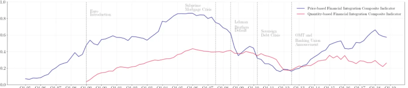
Figure 1: Quarterly data on price- and quantity-based financial integration composite indicator for the Euro Area. Notes: Increases in the indicators
signal greater financial integration. The indicators vary between 0 and 1, with 0 meaning full fragmentation and 1 full integration. Relevant events that may help understanding the evolution of the indicators are noted in the figure.
Hoffmann et al.(2019) argue that these indicators allow to infer equivalent conclusions in regards to the state of financial integration within the Euro Area throughout the years. Based on Figure1, we infer that the price-based financial integration composite indicator shows greater fluctuations in comparison with the quantity-based financial integration composite indicator. A possible reason for this is the fact that financial asset prices, which are on the basis of this indicator, tend to reflect new information rather quickly. Still, the information that each indicator comprises seems to be similar, thereby, the decision on which one to choose to represent financial integration is based on the difference in terms of frequency of observation. The price-based indicator has monthly frequency, while the quantity-based indicator has quarterly frequency, thus the first one is employed.
The price-based financial integration composite indicator is built on measures of cross-country asset return dispersion, e.g. cross-country standard deviation of given interest rates, for which a greater dispersion implies a lower level of financial integration. This instrument is obtained through the aggregation of composite subindices of the main financial market segments (i.e. money market, bond market, equity market and banking market) by computing market size-weighted averages of the respective subindices.
We investigate the proposed premise by considering two distinct scenarios in regards to the level of financial integration, thereby, we build a dummy representative of the level of financial integration, using the values of price-based financial integration composite indicator. For values
greater than or equal to 0.4, the "integration" dummy assumes the value of 1, otherwise is equal to 0. Note that when the dummy assumes the value of 0, we consider to be in the scenario of low-level financial integration. For the remaining cases, in which the dummy equals 1, we consider to be in the scenario of high-level financial integration.
The threshold value assigned to the dummy of 0.4 corresponds to the rounded value of price-based financial integration composite indicator at the moment of the Euro introduction in January 1999, that was followed by a constant rise in financial integration - Figure2. There was a reversion of this tendency with the subprime mortgage crisis in 2007 and further with the sovereign debt crisis, pushing the level of financial integration back to values below 0.4, only registered prior to the Euro introduction. Hence, we consider to be reasonable to assume the value of 0.4, as a reference to characterize the scenarios taken into consideration.
Figure 2: Monthly data on price-based financial integration composite indicator for the Euro Area. Notes: The blue shaded area corresponds to the
period of financial fragmentation represented by the scenario of low-level financial integration ("integration" dummy equals to 0). The grey shaded area corresponds to the period under analysis - March 2002 until December 2018.
3.2 Dependent Variables: Inflation and Output
The key economic variables, that are in this context the dependent variables, correspond to inflation and output. For inflation is used data on Harmonized Index of Consumer Prices (HICP) for each country part of the Euro Area retrieved from Eurostat, nonseasonally nor calendar adjusted data, with reference year 2015=100. In the case of output is employed data on volume index of Production in Industry for each member state retrieved from Eurostat, seasonally and calendar adjusted, with reference year 2015=100. Note that inflation and output are transformed into logarithmic form, so that we obtain the impulse responses in percentage terms.
3.3 Control Variables: Subprime Mortgage Crisis and Sovereign Debt Crisis
We build two dummies, as an effort to control for relevant events that occurred during the period under analysis. The "subprime" dummy aims to control for the subprime mortgage crisis and equals to 1 for the months of July 2007 through March 2010, and 0 otherwise. The "sovereign" dummy is representative of the sovereign debt crisis, assuming the value of 1 for the months of April 2010 through September 2012, and 0 otherwise.
Figure 3: Monthly data on price-based financial integration composite indicator for the Euro Area. Notes: The green shaded area represents the
period for which the "subprime" dummy equals to 1. The orange shaded represents the period for which the "sovereign" dummy equals to 1. The grey shaded area corresponds to the period under analysis - March 2002 until December 2018.
3.4 Monetary Policy
There is a growing literature that investigates the puzzling findings on the effects of central bank announcements on the economy. Romer and Romer(2000) are among the pioneers that identify central bank information effects as the key to solve this puzzle. The authors assume that central bank announcements convey information about their evaluation on the economic outlook in addition to monetary policy decisions. Hence, in a scenario that the central bank paints an economic outlook more favorable than the one anticipated by the general public, a tightening monetary policy triggers the natural increase in real interest rates as well as the contradictory effects at the puzzle’s core, i.e. a decline in the expected unemployment, an increase in output growth and inflation expectations, and a rise in stock prices.
We retrieve data fromKerssenfischer(2019) for the representative variable of monetary policy. The author uses the changes in the 2-year German government bond yield around ECB announce-ments to represent the "policy news" shocks. According to Hanson and Stein (2015), this is a reliable instrument to reflect the path of monetary policy - Figure4.
Figure 4: "Policy News" shocks and "Pure Policy" shocks identified inKerssenfischer(2019).
The author proceeds to explain that an increase in the yield of 2-year German government bonds after an ECB announcement does not necessarily signal a contractionary monetary decision, in the case that information effects are relevant, since it would instead be a consequence of the better-than-expected evaluation on the economic outlook by the ECB.
By acknowledging the existence of these two causes to a "policy news" shock, the author proceeds to disentangle the "pure policy" shock from the "central bank information" shock based on the procedure described inJarocinski and Karadi(2018), thereby, by imposing sign restrictions on the high-frequency comovement of yields and stock prices. The "pure policy" shock is considered to raise yields and lower stock prices, as a result of a higher discount rate and lower expected dividends, while the "central bank information" shock is assumed to raise yields as well as stock prices, given that is reflecting a better-than-expected economic outlook.
Since we investigate the responses to a monetary shock, meaning a shock that derives solely from the monetary component of ECB announcements, the data employed for the monetary policy is "pure policy" shocks.
4
Methodology
This section provides further explanation on the procedure followed to investigate the impact of the level of financial integration within the Euro Area on the transmission mechanism of monetary policy.
4.1 The Model: Local Projection
The model selected to study the proposed premise is local projection developed by Jordà(2005). The author argues that this technique is a strong opponent to the traditional macroeconometric method, i.e. vector autoregressive (VAR), first introduced inSims(1980). Jordà(2005) introduces local projection as an innovative method, that contrary to VAR, does not require the specification nor estimation of the underlying multivariate dynamic system, thereby, we are able to compute the response of variables to shocks at different horizons without imposing many structural restrictions.
According to the author, when projecting 𝑦𝑡+𝑠onto the linear space generated by (𝑦𝑡−1, 𝑦𝑡−2, ..., 𝑦𝑡−𝑝) 0,
one reaches the collection of ℎ regressions as follows:
𝑦𝑡+𝑠 = 𝛼 𝑠 + 𝐵𝑠+1 1 𝑦𝑡−1+ 𝐵 𝑠+1 2 𝑦𝑡−2 + ... + 𝐵 𝑠+1 𝑝 𝑦𝑡− 𝑝+ 𝑢 𝑠 𝑡+𝑠 for s = 0, 1, ..., h
(1)
where 𝛼𝑠is an 𝑛 x 1 vector of constants and 𝐵𝑠+1
𝑖 are matrices of coefficients for each lag 𝑖 and horizon 𝑠 + 1.
Jordà(2005) further argues that this method is an advantageous alternative, given that allows estimation through simple least squares; is robust to misspecification of the data generating process; the appropriate individual or joint inference is simple; and allows an analysis with highly nonlinear and flexible specifications.
The decisive factor in the decision on which method to employ to investigate the proposed premise is related to the last advantage mentioned by the author. Indeed, we intend to compute the impulse responses of certain variables to a shock, under two distinct scenarios, that are determined by a switching variable, which in the particular case of this paper is a binary variable. This implies that we have to use a model, that allows to conduct an analysis with nonlinear specifications in order to reach the impulse responses for each of the described scenarios.
In the case of flexible local projections, one attains the collection of ℎ regressions by extending the local projections in equation1with polynomial terms on 𝑦𝑡−1:
𝑦𝑡+𝑠 = 𝛼𝑠 + 𝐵𝑠+1 1 𝑦𝑡−1+ 𝑄 𝑠+1 1 𝑦2𝑡−1+ 𝐶 𝑠+1 1 𝑦3𝑡−1 + 𝐵 𝑠+1 2 𝑦𝑡−2 + ... + 𝐵 𝑠+1 𝑝 𝑦𝑡− 𝑝+ 𝑢 𝑠 𝑡+𝑠 for s = 0, 1, ..., h
(2)
where the author does not allow for cross-product terms so that 𝑦2𝑡−1 = (𝑦2 1,𝑡−1, 𝑦 2 2,𝑡−1, ..., 𝑦 2 𝑛,𝑡−1) 0
for a matter of choice and parsimony rather than as a requirement. Note that these nonlinear estimates can be easily calculated by least squares, equation by equation.
4.2 The Analysis: Panel Data Local Projection
The analysis is conducted using a local projection model on panel data, which allows to comprise an extensive data set (a total of 3,838 observations), since each member of the Euro Area (a total of 19 countries) are considered individually for the period under analysis, i.e from March 2002 through December 2018 (a total of 202 periods).
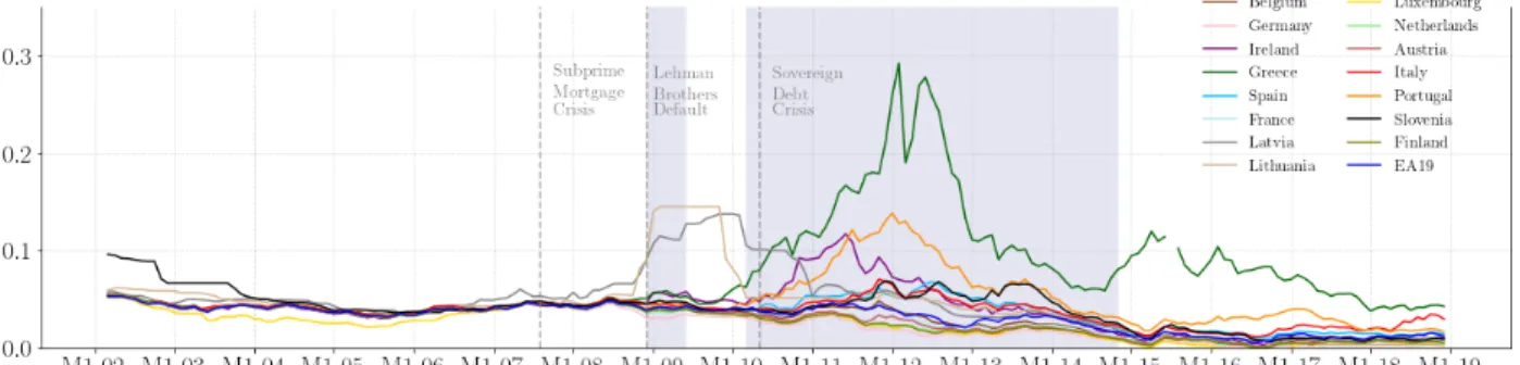
Figure 5: Long-term interest rates for each member state of Euro Area. Notes: The blue shaded area corresponds to the period of financial
fragmentation represented by the scenario of low-level financial integration ("integration" dummy equals to 0). Relevant events that may help understanding the evolution of this variable are noted in the figure. There is no data available for Cyprus, Estonia, Malta and Slovakia. There is a missing value for Greece in July 2015.
We argue that may be of interest assessing a specific group of countries, that stood out during the global economic collapse for diverging greatly from the Euro Area average. Based on Figure 5, we observe that during this critical time, there was the decoupling of the long-term interest rates of the Euro Area with some countries registering significantly higher interest rates than the average of the 19 members states. Indeed, while the Euro Area average was registering values of around 4%, countries like Greece, for the same period, reached alarming values of around 29%. Hence, we conduct an analysis based on subsamples with the first step being to split the 19 members states into two subsamples: core countries and periphery countries. The periphery countries correspond to Greece, Ireland, Italy, Latvia, Lithuania, Portugal, Slovenia and Spain (a total of 1,616 observations) and the core countries correspond to all remaining member states (a total of 2,222 observations).
under two distinct scenarios. The first scenario represents the situation in which there is a low-level of financial integration within the Euro Area, while the second scenario represents the situation in which there is high-level of financial integration within the Euro Area.
4.2.1 Target Group: Each Member of EA19
The initial analysis focus on each member state and consists in computing the impulse responses of inflation and output, using local projection method on panel data. For obtaining the nonlinear responses of the dependent variables, we estimate the following equations:
𝑙_ℎ𝑖𝑐 𝑝𝑖 , 𝑡+ℎ = 𝛼𝑖 , ℎ + 𝛽 𝐴 ℎ ,𝑖𝑠 ℎ𝑜𝑐 𝑘_𝑠1𝑖 , 𝑡 + 𝛽 𝐵 ℎ ,𝑖𝑠 ℎ𝑜𝑐 𝑘_𝑠2𝑖 , 𝑡 + 𝛽 𝐶 ℎ ,𝑖𝑠𝑢 𝑏 𝑝𝑟 𝑖 𝑚 𝑒_𝑠1𝑖 , 𝑡+ + 𝛽𝐷 ℎ ,𝑖 𝑠𝑢 𝑏 𝑝𝑟 𝑖 𝑚 𝑒_𝑠2𝑖 , 𝑡 + 𝛽 𝐸 ℎ ,𝑖𝑠𝑜𝑣 𝑒𝑟 𝑒𝑖𝑔𝑛_𝑠1𝑖 , 𝑡 + 𝛽 𝐹 ℎ ,𝑖 𝑠𝑜𝑣 𝑒𝑟 𝑒𝑖𝑔𝑛_𝑠2𝑖 , 𝑡 + 𝜇𝑖 , 𝑡+ℎ for h = 0, 1,..., H (3) 𝑙_𝑖 𝑝𝑖 , 𝑡+ℎ = 𝜖𝑖 , ℎ + 𝜆 𝐴 ℎ ,𝑖 𝑠 ℎ𝑜𝑐 𝑘_𝑠1𝑖 , 𝑡 + 𝜆 𝐵 ℎ ,𝑖 𝑠 ℎ𝑜𝑐 𝑘_𝑠2𝑖 , 𝑡 + 𝜆 𝐶 ℎ ,𝑖𝑠𝑢 𝑏 𝑝𝑟 𝑖 𝑚 𝑒_𝑠1𝑖 , 𝑡 + + 𝜆𝐷 ℎ ,𝑖𝑠𝑢 𝑏 𝑝𝑟 𝑖 𝑚 𝑒_𝑠2𝑖 , 𝑡 + 𝜆 𝐸 ℎ ,𝑖𝑠𝑜𝑣 𝑒𝑟 𝑒𝑖𝑔𝑛_𝑠1𝑖 , 𝑡 + 𝜆 𝐹 ℎ ,𝑖𝑠𝑜𝑣 𝑒𝑟 𝑒𝑖𝑔𝑛_𝑠2𝑖 , 𝑡 + 𝜃𝑖 , 𝑡+ℎ for h = 0, 1,..., H (4)
The first step into the panel analysis is to define the type of panel model and the effects to be introduced into the model. The model estimated is a fixed-effects model with individual effects based on a within-group estimation technique. The choice of model type results from the need of having a country-specific intercept to capture heterogeneities across countries. This way, it is possible to account for any omitted variables that are not being accounted, while making sure that they are correlated with other variables included in the model. Note that the individual effects introduced in the model can generate an endogeneity, that may lead to producing biased estimates. Hence, we use a within-group approach to eliminate the individual effects before estimation.
Following this, we proceed to identify the remaining parameters based on which the impulse response functions are computed. We start by constructing the data frame that is used as the panel data set. This data set must contain, besides the variable denoting the cross section and the variable denoting the time section, the endogenous variable, the exogenous data (if any), the shock and the switching variable. Starting with the endogenous variable, in the particular case of this paper, we have two endogenous variables, meaning we are assessing the responses of two variables to a given
shock, i.e. inflation and output. Note that we obtain the impulse responses of each endogenous variables separately through the estimations of the equations3and4.
As previously explained, the period under analysis comprises events that may be important to control for, namely the subprime mortgage crisis and the sovereign debt crisis. Hence, the "subprime" dummy and "sovereign" dummy are included as exogenous data with contemporaneous effect, which implies that are not included lags of these variables.
Concerning the shocks, as mentioned in Section 3, we employ the "pure policy" shocks in Kerssenfischer(2019). These shocks have the advantage of being clean of any other effects deriving from ECB announcements besides the monetary policy decisions.
Lastly, we need to identify the switching variable, that is an essential component of the analysis, given that allows to obtain the impulse responses under distinct scenarios. In this case, the switching variable corresponds to the "integration" dummy, meaning that based on this variable we are able to obtain the impulse responses for each scenario considered.
In relation to the best lag-length of the endogenous data, as argued byBrugnolini(2018), there is still lack of clear criteria for local projection method. Still, due to computation restrictions related to the econometric software used, we are not able to select the desired number of lags to be included. Indeed, this decision is made solely by the econometric software and the information on the number of lags included and the criteria used is not disclosed.
In terms of the estimation method for the robust standard errors, we employ the Driscoll and Kraay estimator, labeled SCC (as in "Spatial Correlation Consistent"). Driscoll and Kraay (1998) adapted the Newey-West estimator to panel data methods. Indeed, the Newey-West standard errors are often employed, when working in a time series context. Newey and West (1987) propose an estimator for time series analysis, that is robust to serial correlation as well as to heteroskedasticity. The hypothesis on the basis of this estimator is that the serial correlation dies out "quickly enough". In a panel data context, we have the Driscoll and Kraay robust standard errors, which take into account the serial correlation between residuals from the same individual in different time periods plus the cross-serial correlation between different individuals in different times and, within the same
period, cross-sectional correlation. Note that this estimator can only be applied, when dealing with fairly large data sets, since we need to ensure that the serial and cross-serial dependence die out "quickly enough" with the T dimension. According to the Monte Carlo simulation conducted in Driscoll and Kraay (1998), the practical minimum is set as 𝑇 > 20 − 25, with the n dimension being irrelevant for this matter. We use a data set that comprises 202 periods, thus we fulfill the requirement to be able to employ the Driscoll and Kraay robust standard errors.
4.2.2 Target Group: Core Countries vs Periphery Countries
We conduct also an analysis based on subsamples, for which the first step is to divide the 19 member states into two groups. The reasoning behind this split relies on the behavior of the long-term interest rates of each country, during the critical time that was the global economic collapse. The periphery countries consist in Greece, Ireland, Italy, Latvia, Lithuania, Portugal, Slovenia and Spain, while the core countries consist in the remaining countries.
The model employed to obtain the impulse responses for each subsample is, similarly to the full sample, a fixed-effects model with individual effects based on a within-group estimation technique. The same parameters in which the impulse response functions rely are employed: the endogenous variables are inflation and output (note that we obtain, as in the case of full sample, the responses of inflation and output separately); the "subprime" dummy and "sovereign" dummy are included as exogenous data with contemporaneous impact; the shock correspond to the "pure policy" shock identified inKerssenfischer(2019); and the switching variable is the "integration" dummy. We face the same computation limitations in regards to the selection of the best lag-length of the endogenous data. Lastly, the same estimation method is used to obtain the robust standard errors, i.e. Driscoll and Kraay estimator, given that the data set in both subsamples comprises a total of 202 periods, similarly to the full sample, which surpasses the practical minimum identified inDriscoll and Kraay (1998).
5
Results
After a careful explanation about the steps that the analysis entails, we proceed to analyze the findings. We look into the results for the full sample and subsamples, while assessing the impulse responses of inflation and output for the two scenarios previously described.
5.1 Target Group: Each Member of EA19
We begin with the findings concerning the impulse responses of inflation and output to a monetary shock computed, while considering each member state of the Euro Area, thereby, considering the full sample.
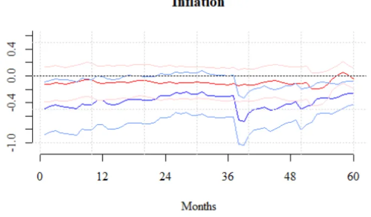
Figure 6: Impulse responses of inflation to a monetary shock through local projection model, while considering the full sample. Notes: The red
line represents the responses in scenario of low-level financial integration. The blue line represents the responses in scenario of high-level financial integration. The remaining lines denote 68% confidence intervals.
Concerning inflation, we observe in Figure 6, that the initial shock, as expected, is different whether a low-level or high-level of financial integration is considered. Starting with the impulse responses in the scenario of low-level financial integration, a monetary shock does not appear to have a strong immediate impact on this variable, since the initial response of inflation is close to 0. For the remaining periods, the responses continue to be close to 0. For the case that is considered to exist a highly integrated financial system, the initial response of inflation to a monetary shock is negative as well as for the remaining periods. According to the monetary theory, this is the expected behavior from inflation, since a tightening monetary policy should lead to a fall in investment
remains unchanged, causes downward pressures on prices to arise.
Looking at the information provided for 6 of the 60 periods in Table1, we infer that the initial response of inflation under the scenario of low-level financial integration to a monetary shock is -0.124%. In contrast, the initial response of inflation under the scenario of high-level financial integration to the same shock is -0.496%. Moreover, the impulse responses of inflation under the scenario of low-level financial integration are of low magnitude, with the strongest response being -0.134% in period 40. When we consider a high-level of financial integration, the strongest response is -0.563%, which is also registered in period 40.
Following this, we proceed to conduct a graphical analysis to assess whether the differences between the impulse responses in each scenario are statistically significant. We infer that the confidence intervals of the impulse responses under the scenario of low-level and high-level financial integration seem to coincide for the majority of the horizons. By looking at the values in Table1, we assess that the "shock_s2", that is, the response of inflation under the scenario of high-level financial integration is statistically significant at a 10% level in period 40. Looking again at Figure 6, we infer that indeed the distance between the impulse responses increases between the 36𝑡 ℎ
and 40𝑡 ℎ period, what explains the confidence intervals to be so close to not coincide during these periods.
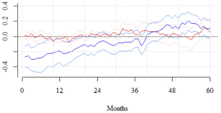
Figure 7: Impulse responses of output to a monetary shock through local projection model, while considering the full sample. Notes: The red
line represents the responses in scenario of low-level financial integration. The blue line represents the responses in scenario of high-level financial integration. The remaining lines denote 68% confidence intervals.
In terms of output, the initial response in each scenario differs, similarly to the case of inflation. For the scenario of low-level financial integration, the initial shock is very close to 0 and the responses
in the remaining horizons are null or at least close to 0. For the scenario of high-level financial integration, the initial response of output to a monetary shock is negative and so is in accordance to the monetary theory. As we move along the horizons, the impulse responses of output continue to be negative, but of increasingly lower magnitude, in absolute terms, until momentarily becoming positive, only to approach again the null response territory. Based on values of Table 1, we infer that the initial response of output under the scenario of low-level financial integration to a monetary shock is 0.017%, while for the scenario of high-level financial integration output falls by 0.273% as result of the same shock.
Looking at Figure7, we infer that the confidence intervals of the impulse responses of output in both the scenario of low-level and high-level financial integration in the first horizons do not coincide, signaling that the responses are statistically different for this period. This is confirmed by the information in Table1, showing that the response under the scenario of high-level financial integration is statistically significant at a 5% level in period 1.
Before comparing the findings with the literature is important to note an interesting result in regards to the dummies included as controls. It appears that we are able to obtain variation not only in periods during which relevant events occurred, such as subprime mortgage crisis, but also in periods in which we do not identify such events. This proves the importance to include such controls that, according to the information in Table1, are statistically significant at different levels for the majority of the periods.
The findings for both inflation and output are in line with the expectations built upon the ideas supported by highly influential names in regards to the Euro project. Indeed,Juncker et al.(2015) as well as any Europhile argue that financial integration is essential, since it ensures that a policy change by the ECB has the desired impact on the European Economy. This implies that the responses across member states are uniform and that, on average, the responses are positive or negative, depending on the monetary policy that the ECB is implementing. Considering this, the results attained match the literature, given that the impulse responses of inflation and output, in the case that there is a low-level of financial integration are close to 0. In contrast, in the scenario that we consider to exist
Table 1: Results for inflation (l_hicp) and output (ln_ip) from estimation with full sample. Notes: This table presents information on the estimated
coefficients, robust standard errors (in parentheses) and statistical significance based on p-value. "_s1" denotes scenario of low-level financial integration and "_s2" denotes scenario of high-level financial integration. This is the information produced by the econometric software used. Information on the intercept is not provided. The absence of sovereign_s2 may be justified by lack of variation of this dummy in scenario of high-level financial integration.
a well structured financial system, the impulse responses of inflation and output are mostly negative, as the economic variables are responding to a tightening monetary policy.
5.2 Target Group: Core Countries vs Periphery Countries
We proceed to conduct further analysis using the local projection model on panel data, while focusing in the impulse responses of two groups chosen strategically. Indeed, the motivation behind this analysis is assessing how the impulse responses of member states that during the global economic collapse diverged greatly from the Euro Area average differ from the impulse responses of the remaining member states.
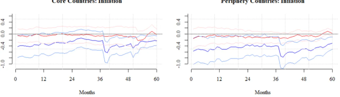
Figure 8: Impulse responses of inflation to a monetary shock through local projection model for core and periphery countries. Notes: The red
line represents the responses in scenario of low-level financial integration. The blue line represents the responses in scenario of high-level financial integration. The remaining lines denote 68% confidence intervals.
are null or close to 0 in all periods for both core and periphery countries. For the scenario of high-level financial integration, the impulse responses are negative for both core and periphery countries, however the magnitude of the responses for the periphery countries is greater. These findings are confirmed by the values in Table2: the initial response of inflation under the scenario of high-level financial integration for core countries is -0.421%, while the initial response of inflation under the same scenario for periphery countries is -0.575%. Moreover, still for the scenario of high-level financial integration, the strongest response, in absolute terms, of core and periphery countries, similarly to the full sample, occur in period 40, and are -0.477% and -0.680%, respectively.
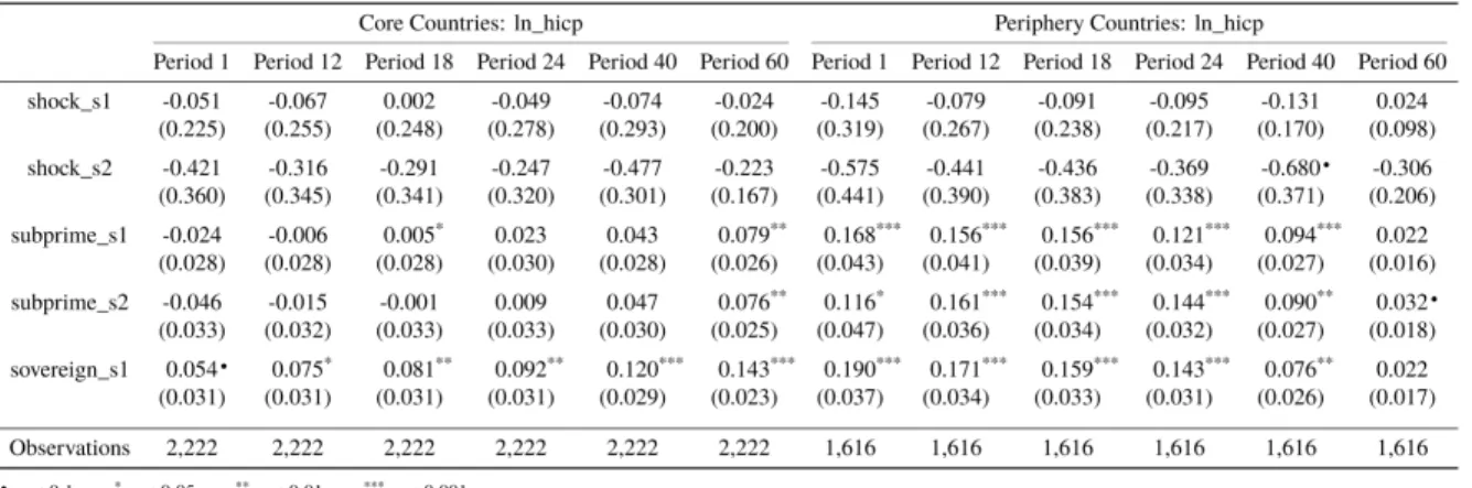
Table 2: Results for inflation (l_hicp) from estimation with subsamples. Notes: This table presents information on the estimated coefficients, robust
standard errors (in parentheses) and statistical significance based on p-value. "_s1" denotes scenario of low-level financial integration and "_s2" denotes scenario of high-level financial integration. This is the information produced by the econometric software used. Information on the intercept is not provided. The absence of sovereign_s2 may be justified by lack of variation of this dummy in scenario oh high-level financial integration.
In terms of statistical significance, based on graphical analysis, for the core countries the con-fidence intervals of the impulse responses seem to always coincide. In contrast, for the periphery countries, we can suspect that the differences between the two scenarios become statistically signif-icant after the 36𝑡 ℎ
period. The values in Table2seem to support these findings, since for the core countries the response under the scenario of high-level financial integration is never statistically sig-nificant and for periphery countries the response under the same scenario is statistically sigsig-nificant at 10% level in period 40. This result is not surprising, given that the periphery countries consist in countries like Greece and Portugal, that during the peak of the global economic collapse, registered values of long-term interest rates considerably higher than the Euro Area average, making these
Figure 9: Impulse responses of output to a monetary shock through local projection model for core and periphery countries. Notes: The red line
represents the responses in scenario of low-level financial integration. The blue line represents the responses in scenario of high-level financial integration. The remaining lines denote 68% confidence intervals.
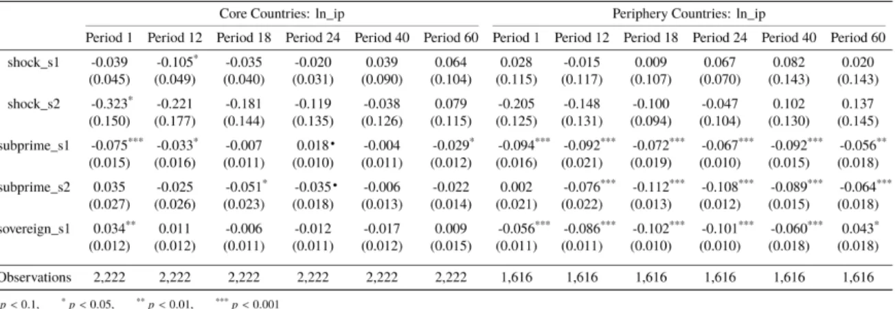
In terms of output, the impulse responses for the scenario of low-level financial integration are, in general, for both subsamples close to 0, despite the periphery countries showing more fluctuation around the null response territory. In the presence of a high-level financial integration, the impulse responses are negative for the majority of the periods. In general, the impulse responses of core countries are smoother than the periphery countries and, contrary to inflation, the core countries show a stronger initial impact under the scenario of high-level financial integration (the initial response under scenario of high-level financial integration for core countries is -0.323% and the initial response under the same scenario for periphery countries is -0.205% - Table3).
Table 3: Results for output (l_ip) from estimation with subsamples. Notes: This table presents information on the estimated coefficients, robust
standard errors (in parentheses) and statistical significance based on p-value. "_s1" denotes scenario of low-level financial integration and "_s2" denotes scenario of high-level financial integration. This is the information produced by the econometric software used. Information on the intercept is not provided. The absence of sovereign_s2 may be justified by lack of variation of this dummy in scenario of high-level financial integration.
Based on the values in Table3, we infer that for core countries the response under the scenario of high-level financial integration is statistically significant at 5% level in period 1. In contrast,
for periphery countries, we do not find that the response under the same scenario is statistically different in any period. This is line with what we observe in Figure 9: the confidence intervals for core countries do not coincide in the first periods, while for periphery countries the confidence intervals appear to always coincide.
One final note is that, similarly to the full sample, we are able to find variation in periods characterized by relevant events, such as the subprime mortgage crisis, as well as in periods for which we do not identify such events. Hence, we confirm also in the case of subsamples, the importance of including such controls and statistical significance at different levels for most of the periods - Table2and3.
The findings for the subsamples, similarly to the full sample analysis, are in line with the literature. The impulse responses for when we assume that there is a low-level of financial integration are null, while in the presence of a high-level of financial integration the impulse responses are different from 0. Hence, we confirm the importance for the Euro Area to have a well structured financial system, since if there is a fragmented financial system, the ECB is not able through its traditional actions to stimulate or restrain the European Economy, depending on what the general economic outlook requires. Moreover, we are able to reach another important result in the case of inflation, as the impulse responses of this variable for periphery countries are of greater magnitude, in absolute terms, than for core countries. This is an interesting result, given that these countries registered considerably higher long-term interest rates, during the global economic collapse, in relation to the Euro Area average. Therefore, a policy change by the ECB, such as pushing the interest rates upwards, would have indeed a greater impact in the economy of these member states.
6
Conclusion
In this paper, we argue that the level of integration of the Euro Area’s financial system affects the functioning of the transmission mechanism of monetary policy. Financial integration is an issue that is on the table, since the creation of the EMU. Relevant figures that were the minds behind
member states to benefit from being part of such economic and financial structure is essential for there to be a strong level of financial integration. Moreover, a crucial consequence of the creation of the EMU is the transferring of the responsibility of conducting the Euro Area monetary policy to the ECB. In order for this institution to be able to fulfill this demanding task, it is necessary to ensure that the effects of a given policy action are uniform across member states.
The financial turmoil triggered by the subprime mortgage crisis was a test to the quality of the integration of the European financial system and it was confirmed what many suspected: financial integration prior to the global financial crisis was weak and incomplete. This resulted in a process of continued fragmentation that contributed to a crisis with a new nature: sovereign debt crisis. For this reason, financial integration is considered to have failed, when it was most needed. Indeed, during this critical time, it was specially important for there to be a highly integrated financial system, such that the ECB could act as a stabilizing authority. In this scenario, the tools at ECB disposal would had been enough to prevent the effects of the subprime mortgage crisis and later on the Lehman Brothers default from becoming unsustainable. This scenario clearly did not materialized, since the ECB was forced to come up with unconventional measures.
We are able to confirm the relation between the level of financial integration and the transmission mechanism of monetary policy. In the case that there is a low-level financial integration, the impulse responses of inflation and output, as anticipated, are null or at least close to 0. This mimics what happened during the financial turmoil and justifies the decision of ECB to resort to unconventional monetary actions. For when we assume to exist a strongly integrated financial system, the impulse responses of inflation and output become negative, making this the ideal scenario for the Euro Area, as the ECB is able to revive the European economy solely through traditional monetary actions. The analysis based on subsamples made this relation even more evident. As expected, in the case of inflation, the responses of the member states that during the global economic collapse did not follow closely the Euro Area average, in terms of long-term interest rates, are of greater magnitude. These are countries that registered considerably high values of long-term interest rate and that, consequently, were more responsive to a policy action conducted by the ECB.
The findings of this paper show that the matter of financial integration, which is of particular interest for the Euro Area, specially in regards to its impact on the functioning of the monetary transmission mechanism, is worth of further investigation.
References
Baele, L., A. Ferrando, P. Hördahl, E. Krylova, and C. Monnet (2004). Measuring Financial Integration in the Euro Area. ECB Occasional Paper (14).
Bernanke, B. S. and M. Gertler (1995). Inside the Black Box: The Credit Channel of Monetary Policy Transmission. Journal of Economic Perspectives 9(4), 27–48.
Brugnolini, L. (2018). About Local Projection Impulse Response Function Reliability. CEIS
Working Paper.
Constâncio, V. (2018). Why EMU requires more Financial Integration. Joint conference of the
European Commission and European Central Bank, Frankfurt am Main(3 May).
Corsetti, G., J. Duarte, and S. Mann (2018). One Money, Many Markets - A factor model approach to monetary policy in the euro area with high-frequency identification. CFM Discussion Paper
Series (CFM-DP2018-05). Centre For Macroeconomics, London, UK..
Draghi, M. (2014). Financial Integration and Banking Union. Conference for the 20th anniversary
of the establishment of the European Monetary Institute, Brussels(12 February).
Driscoll, J. C. and A. C. Kraay (1998). Consistent Covariance Matrix Estimation with Spatially Dependent Panel Data. Review of Economics and Statistics 80(4), 549–559.
ECB (2018). Financial Integration in Europe. ECB Publications on Financial stability.
Eijffinger, S. C. W. and J. de Haan (2000). European Monetary and Fiscal Policy. Oxford: Oxford University Press.
Fecht, F., H. P. Grüner, and P. Hartmann (2007). Welfare Effects of Financial Integration. Financial
Economics(6311), 3–36.
Gürkaynak, R., B. Sack, and E. Swanson (2004). Do Actions Speak Louder Than Words? The Response of Asset Prices to Monetary Policy Actions and Statements. FEDS Working Paper (66). Hanson, S. G. and J. C. Stein (2015). Monetary Policy and Long-Term Real Rates. Journal of
Financial Economics 115(3), 429–448.
Hartmann, P. and F. Smets (2018). The first twenty years of the European Central Bank: Monetary Policy. ECB Working Paper Series, No. 2219 (2219).
Iacoviello, M. and G. Navarro (2019). Foreign Effects of Higher U.S. Interest Rates. Journal of
International Money and Finance 95, 232–250.
Jarocinski, M. and P. Karadi (2018). Deconstructing Monetary Policy Surprises: The Role of Information Shocks. ECB Working Paper (2133).
Jordà, Ò. (2005). Estimation and Inference of Impulse Responses by Local Projections. American
Economic Review 95(1), 161–182.
Jordà, Ò., J. D. Angrist, and G. Kuersteiner (2013). Semiparametric Estimates of Monetary Effects: String Theory Revisited. National Bureau of Economic Research.
Jordà, Ò., M. Schularick, and A. M. Taylor (2019). The Effects of Quasi-Random Monetary Experiments. Journal of Monetary Economics.
Juncker, J.-C., D. Tusk, J. Dijsselbloem, M. Draghi, and M. Schulz (2015). Completing Europe’s Economic and Monetary Union.
Kerssenfischer, M. (2019). Information Effects of Euro Area Monetary Policy: New Evidence from High-Frequency Futures Data. Deutsche Bundesbank Discussion Paper.
Lagarde, C. (2019). The Euro Area: Creating a Stronger Economic Ecosystem. Banque de France,
Paris(March 28).
Lamfalussy, A. (2009). The Specificity of the Current Crisis. Revue de la Banque/Bank- en
Financiewezen July(5), 279–283.
Millo, G. (2017). Robust Standard Error Estimators for Panel Models: A Unifying Approach.
Journal of Statistical Software 82(3).
Mishkin, F. S. (1995). Symposium on the Monetary Transmission Mechanism. Journal of Economic
Perspectives 9(4), 3–10.
Nardo, M., F. Pericoli, and P. Poncela (2017). Risk-sharing among European Countries. Publications
Office of the European Union.
Newey, W. and K. West (1987). A Simple, Positive Semi-Definite, Heteroscedasticity and Autocor-relation Consistent Covariance Matrix.
Romer, C. D. and D. H. Romer (2000). Federal Reserve Information and the Behavior of Interest Rates. American Economic Review 90(3), 429–457.
Sims, C. A. (1980). Macroeconomics and Reality. Econometrica 48(1), 1–48.
Stiglitz, J. E. (2010). Risk and Global Economic Architecture: Why Full Financial Integration May Be Undesirable. National Bureau of Economic Research.
Taylor, J. B. (1995). The Monetary Transmission Mechanism: An Empirical Framework. Journal