Carlos Pestana Barros & Nicolas Peypoch
A Comparative Analysis of Productivity Change in Italian and Portuguese Airports
WP 006/2007/DE _________________________________________________________
António Afonso & Ricardo M. Sousa
Consumption, Wealth, Stock and Government
Bond Returns: International Evidence
WP 09/2011/DE/UECE
Department of Economics
WORKING PAPERS
ISSN Nº 0874-4548
School of Economics and Management
TECHNICAL UNIVERSITY OF LISBONConsumption, Wealth, Stock and Government
Bond Returns: International Evidence
*
António Afonso
a, $,#, and Ricardo M. Sousa
b aISEG/TULisbon, Technical University of Lisbon, Department of Economics, UECE - Research Unit on Complexity and Economics, R. Miguel Lupi 20, 1249-078 Lisbon, Portugal.
European Central Bank, Directorate General Economics, Kaiserstraße 29, D-60311 Frankfurt am Main, Germany
b
University of Minho, Department of Economics and Economic Policies Research Unit (NIPE), Campus of Gualtar, 4710-057 - Braga, Portugal.
London School of Economics, Financial Markets Group (FMG), Houghton Street, London WC2 2AE, United Kingdom.
Abstract
In this paper, we show, from the consumer’s budget constraint, that the residuals of the trend relationship among consumption, aggregate wealth, and labour income should predict both stock returns and government bond yields. We use data for several OECD countries and find that when agents expect future stock returns to be higher, they will temporarily allow consumption to rise. Regarding government bond yields, when bonds are seen as a component of asset wealth, then investors react in the same way. If, however, the increase in the yields is perceived as signalling a future rise in taxes, then they will temporarily reduce their consumption.
JEL classification: E21, E44, D12.
Keywords: consumption, wealth, stock returns, bond returns.
*
We are grateful to Jerry Coakley, Ad van Riet, to participants to an ECB workshop, to the Money, Macro and Finance Research Group 41st Annual Conference, and to two anonymous referees for helpful comments. Ricardo Sousa would like to thank the Fiscal Policies Division of the ECB for its hospitality. The opinions expressed herein are those of the authors and do not necessarily reflect those of the ECB or the Eurosystem.
$
Corresponding author. European Central Bank, Directorate General Economics, Kaiserstraße 29, D-60311 Frankfurt am Main, Germany. E-mail addresses: antonio.afonso@ecb.europa.eu, aafonso@iseg.utl.pt (A. Afonso), rjsousa@eeg.uminho.pt, rjsousa@alumni.lse.ac.uk. (R. Sousa).
#
Contents
1. Introduction ... 3
2. Theoretical framework and empirical methodology... 5
2.1 Theory ... 5
2.2. Long-run relationship between consumption, wealth and income ... 7
3. Empirical results ... 10
3.1. Forecasting stock returns... 10
3.2. Forecasting government bond returns ... 13
3.3. Forecasting consumption growth... 17
4. Robustness analysis ... 19
4.1. Additional control variables ... 19
4.2. Nested forecast comparisons ... 22
5. Conclusion... 23
1. Introduction
Differences in expected returns across assets are explained by differences in risk, and the risk premium is generally considered as reflecting the ability of an asset to insure against consumption fluctuations (Sharpe, 1964). Despite this belief, a measure such as the covariance of returns across portfolios and contemporaneous consumption growth did not prove to be sufficient to explain the differences in expected returns (Breeden et al., 1989). In fact, the literature on asset pricing has concluded that inefficiencies of financial markets1 and the rational response of agents to time-varying investment opportunities2 help justifying why expected excess returns appear to vary with the business cycle.
In addition, different macro-financially motivated variables that capture time-variation in expected returns have been developed. For instance: the consumption-wealth ratio (Lettau and Ludvigson, 2001); the long-run risk (Bansal and Yaron, 2004; Bansal et al., 2005); the labour income risk (Julliard, 2004); the housing collateral risk (Lustig and van Nieuwerburgh, 2005);3 the ultimate consumption risk (Parker and Julliard, 2005); and the composition risk (Yogo, 2006; Piazzesi et al., 2007). Additional variables include the (adjusted) dividend or cash flow yield (Goyal and Welsh, 2003; Robertson and Wright, 2006; Boudoukh et al., 2007); the ratio of excess consumption (i.e. consumption in excess of labour income) to observable assets (Whelan, 2008); and the wealth composition risk (Sousa, 2010a).4
In contrast with the literature on the predictability of stock returns, only a few studies tried to explain the factors behind sovereign bond risk premia. Among these: Fama and Bliss (1987) focus on the spread between the n-year forward rate and the one-year yield; Campbell and Shiller (1991) emphasize the Treasury yield spreads; Campbell and Cochrane (1999) and Wachter (2006) stress the role of shocks to aggregate consumption, while Brandt and Wang (2003) address the importance of shocks to inflation; Cochrane and Piazzesi (2005) highlight a single factor, a single tent-shaped linear combination of forward rates; and Ludvigson and Ng (2009) find marked countercyclical variation in bond risk premia.
The current paper argues that the wealth and macroeconomic data can be combined to address the issue of predictability of asset returns. More specifically, we derive an
1
See Fama (1998), Fama and French (1996), and Farmer and Lo (1999).
2
See Sundaresan (1989), Constantinides (1990), Campbell and Cochrane (1999), Duffee (2005), and Santos and Veronesi (2006).
3 In the same spirit, Sousa (2007a) shows that housing can be used as an hedge against wealth shocks.
4
Sousa (2007b) provides a comparison of the forecasting power of several empirical proxies, but distinguishes between their expected and unexpected components.
equilibrium relation between the transitory deviation from the common trend in consumption, aggregate wealth and labour income, labelled as cay (cday when disaggregate wealth is used) and stock returns as well as government bond yields.
The above-mentioned common trends summarize agent's long-term expectations of stock returns, government bond yields and/or consumption growth. In particular, when forward-looking investors expect future stock returns to be higher, they will allow consumption to rise above its common trend with aggregate wealth and labour income. As in Lettau and Ludvigson (2001) and Sousa (2010a), in this way, investors insulate future consumption from fluctuations in stock returns. As for government bond returns, one needs to understand the way government debt is perceived by agents. If government bonds are seen as a component of asset wealth, then investors allow consumption to rise above its equilibrium relationship with aggregate wealth and labour income when they have expectations of higher government bond yields. However, if the issuance of government debt is seen as a symptom of deteriorating public finances, then investors will allow consumption to fall below its common trend with aggregate wealth and labour income.
Using data for a set of 16 OECD countries, we show that the predictive power of the cay and cday measures for real stock returns is particularly important for horizons from three to four quarters for Australia, Belgium, Canada, Denmark, Finland, the UK and the US. As for Germany, Ireland, and Spain, those proxies do not seem to track well time-variation in stock returns.
In what concerns government bond returns, our analysis suggests that we can cluster the countries in two groups. In the first group (which includes Australia, Finland and the Netherlands), both cay and cday have an associated coefficient with positive sign in the forecasting regressions. Therefore, this corroborates the idea that government debt is a component of asset wealth. In the second group (which includes Canada, Denmark, Germany, Ireland, Italy and the US), the forecasting regressions show that both cay and
cday have an associated negative coefficient. Consequently, agents in these countries
understand the rise in government bond returns rather as signalling an increase in future taxation.
Finally, assessing the robustness of our results, we show that: (i) additional control variables do not change the predictive power of cay and cday; and (ii) models that include
cay and cday perform better than other benchmark models.
The paper is organized as follows. Section two describes the theoretical framework and presents the empirical methodology. Section three provides the estimation results of
the forecasting regressions for asset returns. Section four provides the robustness analysis. Section five concludes.
2. Theoretical framework and empirical methodology 2.1 Theory
Consider the case of a representative consumer. The budget constraint can be written as ), )( 1 ( , 1 1 wt t t t R W C W (1)
where Wt represents aggregate wealth, Ct denotes private consumption, and Rw,t+1 corresponds to the return on aggregate wealth between period t and t+1.
Campbell and Mankiw (1989) show that, under the assumption that the consumption-aggregate wealth is stationary and that limi wi(cti wti)0,5 one can approximate equation (1) by a Taylor expansion as follows
, 1 1 , i i t t w w t i w t i w i i c w r c k
(2) where c logC, w logW, and kw is a constant. This equation shows that deviations of consumption from its equilibrium relationship with aggregate wealth can reflect changes in the returns on aggregate wealth or in consumption growth.The aggregate return on wealth can be decomposed as
, 1 , 1 (1- ) , 1,
w t t a t t h t
R R R (3) where is a time varying coefficient and Rt a,t+1 is the return on asset wealth. Campbell
(1996) shows that the last expression can be approximated as
, , (1- ) , ,
w t t a t t h t r
r r r k (4) where kr is a constant, and rw,t is the log return on asset wealth. Similarly, the log total wealth can be approximated as
t (1- )ht ,
t a
w a k (5) where at is the log asset wealth, ht is the log human wealth, ω is the mean of , and kt a is a
constant.
Campbell (1996) and Jagannathan and Wang (1996) suggest that labour income,
Yt, can be thought as the dividend on human capital, Ht. Consequently, the return to human capital can be defined as:
5
. 1 1 1 1 , t t t t h H Y H R (6)
Log-linearizing this relation around the steady state,6 one gets
, 1 (1- ) ( 1- 1) - ( - ) 1,
h t h h h t t t t t
r k h y h y y (7)
where r log(1+R), h logH, y logY, kh is a constant of no interest, and the variables without time subscript are evaluated at their steady state value. Assuming that
, 0 ) (
limi hi hti yti the log human capital income ratio can be rewritten as a linear combination of future labour income growth and future returns on human capital:
1 , 1 - i ( - ) . t t h t i h t i h i h y y r k
(8) Replacing equation (4), (7) and (8) into (2), one obtains
) )( 1 ( 1 i t 1 i i h t t t a y y c , ) ( ) 1 ( 1 i t 1 i t h, 1 1 i t a, r c k r i i w i i h i w i i w
(9)where k is a constant. This equation holds ex-post as a direct consequence of agent's budget constraint, but it also has to hold ex-ante. Taking time t conditional expectation of both sides gives
, c y ) 1 ( ) -(1 -1 i t 1 i t 1 1 i t a, E E k r E y a c t i i w t i i h t i i w t cay t t t t
(10) where (1 ) ( ) , 1 i t h, 1
i i h i w t r is a stationary component.When the left hand side of equation (10) is high, consumers expect high future returns on market wealth. Based on that equation, cayt may carry relevant information about market expectations of future asset returns, ra,t+i, future labour income growth,
i t
y
, and future consumption growth, cti. In particular, when future stock returns are
expected to be higher, forward-looking investors will allow consumption to rise above its common trend with aggregate wealth and labour income. In what concerns government bond returns: (i) investors behave in the same fashion when government bonds are seen as
6 This is true under the assumption that the steady state human capital-labour income ratio is constant, that is, Y H/ h1 1
a component of asset wealth; but (ii) investors will reduce consumption when higher government bond returns are perceived as signalling a deterioration of public finances.
Finally, Sousa (2010a) highlights the importance of wealth composition in pricing risk premium.7 By disaggregating wealth, at, into its major components (financial wealth,
ft, housing wealth, ut) and aggregate returns, ra,t, into returns on financial assets, rf,t, and returns on housing assets, ru,t, one can link the trend deviation cdayt with the market expectations of future financial and housing asset returns as follows:
t cday t u f t u t f t f u y c -(1- ) , c y ) -1 ( 1 i t 1 i t 1 1 i t u, 1 i t f, E r E E k r E t i i w t i i h t u f i i w t u i i w t f
(11) where (1 ) ( ) . 1 i t h, 1
i i h i w u f t r 82.2. Long-run relationship between consumption, wealth and income
In order to assess the long-run relationship between consumption, (dis)aggregate wealth and labour income, we start by using the augmented Dickey-Fuller and the Phillips-Perron tests. This allows one to determine the existence of unit roots in the series and the tests suggest that all series are first-order integrated, I(1). Next, we analyze the existence of cointegration among the series, using the methodology of Engle-Granger and Phillips-Ouliaris, and find evidence that supports that hypothesis. Finally, we estimate the trend relationship among consumption, wealth and labour income following Davidson and Hendry (1981) and Blinder and Deaton (1985).
Since the impact of different assets’ categories on consumption can vary (Poterba and Samwick, 1995; Sousa, 2008), we also disaggregate wealth into its main components: financial wealth and housing wealth. Following Stock and Watson (1993), we use a dynamic least squares (DOLS) technique, specifying the following equation
7
Sousa (2010b) also shows that monetary policy can indeed have a strong impact on the composition of wealth in the euro area as a whole.
8
From a theoretical point of view, some authors argue that housing wealth effects should be small. For instance, Buiter (2008) sustains that an increase in value of housing leads to higher housing consumption costs, which offset the housing wealth effect on non-housing consumption. Muellbauer (2008) suggests that the positive effect on non-housing consumption from an increase in housing prices is counterbalanced by a fall on housing consumption. Calomiris et al. (2009) emphasize that changes in housing wealth are typically correlated with changes in expected permanent income.
t k k i i y k k i i a t y t a t a y b a b y c
i -t , i -t , (12)where the parameters and a represent, respectively, the long-run elasticities of y
consumption with asset wealth and labour income, Δ denotes the first difference operator,
is a constant, and is the error term. t
In the estimation of the long-run relationships among consumption, (dis)aggregate wealth and labour income, we use quarterly data, post-1960, for 16 countries (Australia, Austria, Belgium, Canada, Denmark, Finland, France, Germany, Ireland, Italy, Japan, the Netherlands, Spain, Sweden, the UK, the US).
The consumption data are the private consumption expenditure and were taken from the database of the NiGEM model of the NIESR Institute, the Main Economic Indicators of the OECD and DRI International. The labour income data correspond to the compensation series of the NIESR Institute. In the case of the US, labour income series was constructed following Lettau and Ludvigson (2004). The wealth data were taken from the national central banks or Eurostat. For the G-8 countries, the wealth series were compared with alternative sources, namely, Bertaut (2002), Pichette and Tremblay (2003), Tan and Voss (2003), Catte et al. (2004), and the Bank of Japan.
The stock return data were computed using the share price index provided by the International Financial Statistics of the IMF and the dividend yield ratio provided by Datastream. The 10-year government bond yield data were obtained from the International Financial Statistics of the IMF.
The government finance data normally refers to the Central Government, therefore, with the exclusion of the Local and/or the Regional Authorities. It is typically disseminated through the monthly publications of the General Accounting Offices, Ministries of Finance, National Central Banks and National Statistical Institutes of the respective countries. The latest figures are also published in the Special Data Dissemination Standard (SDDS) section of the International Monetary Fund (IMF) website.
Finally, the population series were taken from the OECD's Main Economic Indicators and interpolated (from annual data), and all series were deflated with consumption deflators and expressed in logs of per capita terms. The series were seasonally adjusted using the X-12 method where necessary and the time frames were chosen based on the availability of reliable data for each country.
Table 1.1 shows the estimates for the shared trend among consumption, asset wealth, and income. It can be seen that, despite some heterogeneity, the long-run elasticities of consumption with respect to aggregate wealth and labour income imply roughly a share of one third for asset wealth and two thirds for human wealth in aggregate wealth, in accordance with the values that one would expect in a production function with Cobb-Douglas technology. This is particularly true for Australia, Canada, Finland, France, Ireland, the UK and the US. Moreover, the disaggregation between asset wealth and labour income is statistically significant for all countries (with the exceptions of Finland and Italy). The table also presents the unit root tests to the residuals of the cointegration relationship based in the Engle and Granger (1987) methodology and reveals their stationarity.
Table 1.1 - Long-run relationship between consumption, aggregate wealth, and labour income. cayt = ct - β1at - β2yt. ADF t-statistic Critical values a Y Lags: 1 5% 10% Australia 0.35*** (13.39) 0.54*** (8.03) -1.45 -1.95 -1.61 Austria -0.08*** (-5.10) 1.46*** (23.48) -2.30 -1.95 -1.61 Belgium 0.16*** (8.02) 0.56*** (13.01) -4.53 -1.95 -1.61 Canada 0.36*** (13.16) 0.56*** (10.82) -2.27 -1.95 -1.61 Denmark 0.09*** (6.12) 0.65*** (19.10) -1.88 -1.95 -1.61 Finland 0.38*** (6.88) 0.13 (0.98) -1.78 -1.95 -1.61 France 0.25*** (16.95) 0.55*** (18.03) -2.09 -1.95 -1.61 Germany 0.13* (1.71) 1.16*** (35.01) -1.64 -1.95 -1.61 Ireland 0.36*** (9.17) 0.46*** (10.03) -3.33 -1.95 -1.61 Italy -0.02 (-0.20) 1.49*** (11.32) -1.07 -1.95 -1.61 Japan 0.08*** (3.74) 0.89*** (25.99) -3.27 -1.95 -1.61 Netherlands 0.17*** (12.92) 0.53*** (10.30) -3.00 -1.95 -1.61 Spain 0.06* (1.67) 0.76*** (16.10) -2.19 -1.95 -1.61 Sweden -0.13** (-2.45) 1.12*** (9.06) -2.06 -1.95 -1.61 UK 0.32*** (13.84) 0.66*** (12.84) -2.45 -1.95 -1.61 US 0.28*** (17.14) 0.79*** (35.75) -2.90 -1.95 -1.61
Notes: Newey-West (1987) corrected t-statistics appear in parenthesis.
*, **, *** denote statistical significance at the 10, 5, and 1% level, respectively.
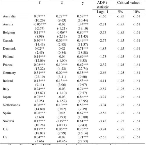
Table 1.2 reports the estimates of the long-run elasticities of consumption with respect to financial wealth, f, housing wealth, u, and labour income. First, it shows that the disaggregation between financial and housing wealth is statistically significant for almost
all countries. Moreover, consumption is, in general, more sensitive to financial wealth than to housing wealth, as the elasticities of consumption with respect to financial wealth are larger in magnitude. Second, it tells us that consumption is very responsive to financial wealth in the case of Belgium (0.11), Canada (0.30), Finland (0.14), Germany (0.31), Italy (0.24), Sweden (0.12) and the UK (0.17). Third, the long-run elasticity of consumption with respect to housing wealth is particularly strong for Australia (0.27), France (0.10), Ireland (0.13) and the Netherlands (0.10). Finally, the cointegration tests suggest that the residuals of the common trend between consumption, financial wealth, housing wealth and labour income are stationary.
Table 1.2 - Long-run relationship between consumption, financial wealth, housing wealth, and labour income. cdayt = ct - β1ft - β2ut - β3yt.
ADF t-statistic Critical values f U y Lags: 1 5% 10% Australia 0.07*** (10.26) 0.27*** (9.63) 0.59*** (10.44) -1.66 -1.95 -1.61 Austria -0.05*** (-2.67) -0.02 (-1.21) 1.44*** (19.10) -2.31 -1.95 -1.61 Belgium 0.11*** (8.98) -0.06** (-2.13) 0.80*** (11.45) -3.73 -1.95 -1.61 Canada 0.30*** (14.43) 0.06*** (2.98) 0.49*** (11.37) -2.77 -1.95 -1.61 Denmark 0.02** (2.45) 0.02 (0.84) 0.71*** (18.88) -1.83 -1.95 -1.61 Finland 0.14*** (12.09) -0.04 (-1.00) 0.69*** (6.53) -1.73 -1.95 -1.61 France 0.08*** (17.22) 0.10*** (4.23) 0.62*** (22.74) -2.32 -1.95 -1.61 Germany 0.31*** (22.10) 0.09*** (3.41) 0.33*** (9.60) -2.66 -1.95 -1.61 Ireland 0.13*** (9.11) 0.13*** (3.06) 0.53*** (9.97) -4.11 -1.95 -1.61 Italy 0.24*** (15.87) -0.03 (-1.10) 0.74*** (9.57) -2.87 -1.95 -1.61 Japan 0.07*** (3.25) -0.03 (-1.52) 0.86*** (13.95) -3.27 -1.95 -1.61 Netherlands 0.08*** (14.80) 0.10*** (0.02) 0.53*** (7.39) -3.04 -1.95 -1.61 Spain 0.08*** (5.60) 0.02 (0.93) 0.67*** (13.80) -2.58 -1.95 -1.61 Sweden 0.12*** (10.28) -0.15*** (-8.11) 0.61*** (9.43) -3.43 -1.95 -1.61 UK 0.17*** (18.87) 0.06*** (2.99) 0.76*** (16.14) -3.94 -1.95 -1.61 US 0.04*** (2.66) -0.02 (-0.46) 1.21*** (22.53) -2.55 -1.95 -1.61
Notes: Newey-West (1987) corrected t-statistics appear in parenthesis.
*, **, *** denote statistical significance at the 10, 5, and 1% level, respectively.
3. Empirical results
3.1. Forecasting stock returns
Equation (10) shows that transitory deviations from the long-run relationship among consumption, aggregate wealth and income, cayt, mainly reflect agents’ expectations of future changes in asset returns.
Moreover, given the disaggregation of asset wealth into its main components (financial and housing wealth), we argue that cdayt should provide a better forecast for asset returns than a variable like cayt in Lettau and Ludvigson (2001). We look at real stock returns (denoted by SRt) for which quarterly data are available and should provide a good proxy for the non-human component of asset wealth.
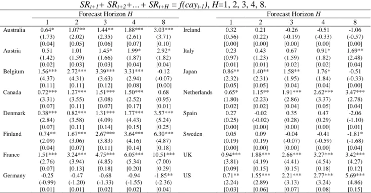
Table 2.1 summarizes the forecasting power of cayt at different horizons. It reports estimates from OLS regressions of the H-period real stock return, SRt+1 + … + SRt+H, on the lag of cayt.
Table 2.1 – Forecasting real stock returns: estimated effect of cay.
SRt+1+ SRt+2+…+ SRt+H = f(cayt-1), H=1, 2, 3, 4, 8.
Forecast Horizon H Forecast Horizon H
1 2 3 4 8 1 2 3 4 8 Australia 0.64* (1.73) [0.04] 1.07** (2.02) [0.05] 1.44** (2.35) [0.06] 1.88*** (2.61) [0.07] 3.03*** (3.71) [0.10] Ireland 0.32 (0.56) [0.00] 0.21 (0.22) [0.00] -0.26 (-0.19) [0.00] -0.51 (-0.33) [0.00] -1.06 (-0.57) [0.00] Austria 0.51 (1.42) [0.02] 1.01 (1.59) [0.03] 1.45* (1.66) [0.03] 1.99* (1.87) [0.04] 2.92* (1.82) [0.04] Italy 0.23 (0.97) [0.01] 0.43 (1.23) [0.01] 0.67 (1.59) [0.02] 0.91* (1.82) [0.02] 1.69** (2.48) [0.04] Belgium 1.56*** (4.37) [0.11] 2.72*** (4.31) [0.11] 3.39*** (3.63) [0.12] 3.31*** (2.94) [0.08] -0.12 (-0.07) [0.00] Japan 0.86** (2.32) [0.05] 1.40** (2.31) [0.05] 1.58** (1.95) [0.04] 1.76* (1.84) [0.04] -0.51 (-0.33) [0.00] Canada 0.72*** (3.31) [0.07] 1.27*** (3.55) [0.11] 1.51*** (3.08) [0.07] 1.50*** (2.52) [0.17] 0.68 (0.95) [0.01] Netherlands 0.65* (1.80) [0.02] 1.15** (2.23) [0.02] 1.91*** (2.86) [0.04] 2.62*** (3.37) [0.05] 3.47*** (2.78) [0.04] Denmark 0.38*** (2.84) [0.07] 0.82*** (3.58) [0.11] 1.31*** (4.09) [0.14] 1.77*** (4.43) [0.15] 3.57*** (5.24) [0.25] Spain 0.27 (0.25) [0.00] -0.02 (-0.02) [0.00] 0.35 (0.28) [0.00] 0.47 (0.29) [0.00] -2.06 (-1.10) [0.01] Finland 0.74** (2.09) [0.04] 1.67*** (3.06) [0.07] 2.67*** (3.83) [0.11] 3.64*** (4.16) [0.14] 6.30*** (4.87) [0.18] Sweden 0.05 (0.19) [0.00] 0.09 (0.19) [0.00] -0.04 (-0.07) [0.00] -0.41 (-0.59) [0.00] -1.81* (-1.68) [0.04] France 1.51*** (2.76) [0.07] 3.24*** (3.94) [0.13] 4.75*** (4.85) [0.18] 6.05*** (5.34) [0.20] 10.51*** (7.00) [0.29] UK 0.94*** (3.81) [0.09] 1.88*** (4.19) [0.15] 2.66*** (4.41) [0.15] 3.27*** (4.54) [0.18] 3.42*** (4.27) [0.12] Germany -0.25 (-0.99) [0.01] -0.47 (-1.20) [0.01] -0.68 (-1.33) [0.02] -0.94 (-1.55) [0.02] -1.85** (-2.36) [0.04] US 0.71** (2.24) [0.03] 1.55*** (2.89) [0.06] 2.21*** (3.13) [0.07] 2.77*** (3.24) [0.08] 5.69*** (4.86) [0.15]
Notes: Newey-West (1987) corrected t-statistics appear in parenthesis. Adjusted R-square is reported in square brackets. *, **, *** denote statistical significance at the 10, 5, and 1% level, respectively.
It shows that cayt is statistically significant for almost all countries and the point estimate of the coefficient is large in magnitude. Moreover, its sign is positive. These results are in line with the theoretical framework presented in Section 3, suggesting that investors will temporarily allow consumption to rise above its equilibrium level in order to smooth it and insulate it from an increase in real stock returns. Therefore, deviations in the long-term trend among ct, at and yt should be positively related to future stock returns.
Moreover, they explain an important fraction of the variation in future real returns (as described by the adjusted R-square), in particular, at horizons spanning from three to four quarters. In fact, at the four quarter horizon, cayt explains 20% (France), 18% (UK), 17% (Canada), 15% (Denmark), 14% (Finland), 8% (Belgium and US) and 7% (Australia)
of the real stock return. In contrast, its forecasting power is poor for countries such as Germany, Ireland, Spain and Sweden.
Table 2.2 summarizes the forecasting power of cdayt at different horizons. It reports estimates from OLS regressions of the H-period real stock return, SRt+1 + … +
SRt+H, on the lag of cdayt.
Table 2.2 – Forecasting real stock returns: estimated effect of cday.
SRt+1+ SRt+2+…+ SRt+H = f(cdayt-1), H=1, 2, 3, 4, 8.
Forecast Horizon H Forecast Horizon H
1 2 3 4 8 1 2 3 4 8 Australia 0.66* (1.67) [0.03] 1.08* (1.92) [0.04] 1.53** (2.19) [0.05] 2.18** (2.47) [0.07] 3.72*** (3.55) [0.10] Ireland 0.37 (0.63) [0.00] 0.34 (0.35) [0.00] -0.08 (-0.06) [0.00] -0.30 (-0.20) [0.00] 0.24 (0.11) [0.00] Austria 0.39 (1.14) [0.01] 0.75 (1.24) [0.01] 1.04 (1.26) [0.02] 1.44 (1.43) [0.02] 2.21 (1.39) [0.02] Italy 0.65 (1.09) [0.01] 1.27 (1.46) [0.02] 1.76* (1.78) [0.02] 2.21* (1.95) [0.03] 5.50*** (3.06) [0.09] Belgium 2.25*** (4.50) [0.18] 4.18*** (5.97) [0.24] 5.74*** (7.15) [0.28] 6.67*** (7.28) [0.26] 6.96*** (4.27) [0.12] Japan 0.80** (2.24) [0.05] 1.33** (2.21) [0.05] 1.58** (1.96) [0.04] 1.77* (1.89) [0.04] -0.31 (-0.18) [0.00] Canada 1.21*** (4.71) [0.07] 2.34*** (5.48) [0.19] 3.08*** (4.95) [0.19] 3.40*** (4.22) [0.17] 3.44*** (3.14) [0.10] Netherlands 0.69* (1.90) [0.02] 1.29** (2.48) [0.03] 2.13*** (3.17) [0.05] 2.90*** (3.69) [0.06] 4.09*** (3.05) [0.05] Denmark 0.36*** (2.61) [0.06] 0.76*** (3.27) [0.10] 1.21*** (3.74) [0.12] 1.62*** (4.07) [0.13] 3.18*** (4.80) [0.21] Spain -0.40 (-0.30) [0.00] 0.04 (0.02) [0.00] 1.76 (0.81) [0.01] 3.84 (1.45) [0.03] 4.91 (1.46) [0.02] Finland 0.92* (1.94) [0.03] 1.68** (2.06) [0.03] 2.27** (2.18) [0.04] 2.74** (2.11) [0.04] 4.01* (1.86) [0.03] Sweden 0.87 (1.58) [0.03] 2.20*** (2.77) [0.08] 3.45*** (3.60) [0.11] 3.98*** (3.68) [0.11] 4.65*** (3.73) [0.08] France 1.83*** (2.87) [0.07] 3.99*** (4.13) [0.14] 5.91*** (5.20) [0.19] 7.70*** (6.04) [0.22] 13.51*** (8.12) [0.32] UK 0.95*** (2.49) [0.06] 2.08*** (4.25) [0.12] 3.13*** (5.30) [0.17] 4.13*** (5.65) [0.22] 5.68*** (4.66) [0.22] Germany -1.52*** (-3.10) [0.06] -2.16*** (-2.65) [0.05] -2.15** (-1.99) [0.03] -2.06 (-1.51) [0.02] 1.19 (0.68) [0.00] US 0.50 (0.88) [0.01] 1.14 (1.38) [0.02] 1.93* (1.79) [0.03] 2.41* (1.93) [0.04] 5.42*** (3.68) [0.09]
Notes: Newey-West (1987) corrected t-statistics appear in parenthesis. Adjusted R-square is reported in square brackets. *, **, *** denote statistical significance at the 10, 5, and 1% level, respectively.
In accordance with the findings for cayt, it shows that cdayt is statistically significant for almost all countries, the point estimate of the coefficient is large in magnitude and its sign is positive. Therefore, deviations in the long-term trend among ct,
ft, ht and yt should be positively linked with future stock returns.
In addition, it can be seen that the trend deviations explain a substantial fraction of the variation in future real returns. At the four quarter horizon, cdayt explains 26% (Belgium), 22% (France and UK), 17% (Canada), 13% (Denmark), 7% (Australia), 6% (Netherlands), 4% (Finland and US) of the real stock return. However, it does not seem to exhibit forecasting power for countries such as Germany, Ireland, and Spain.
Noticeably, it is important to emphasize that, in general, cdayt performs better than
cayt, also in accordance with the findings of Sousa (2010a), reflecting the ability of cdayt to track the changes in the composition of asset wealth. Portfolios with different compositions of assets are subject to different degrees of liquidity, taxation, or transaction
costs. For example, agents who hold portfolios where the exposure to housing wealth is larger face an additional risk associated with the (il)liquidity of these assets and the transaction costs involved in trading them. Wealth composition is, therefore, an important source of risk that cdayt – but not cayt – is able to capture.
3.2. Forecasting government bond returns
We now look at the power of cayt (Table 3.1) and cdayt (Table 3.2) in predicting bond returns (proxied by the government bond yields and denoted by BRt) for which quarterly data are available. As mentioned before, one needs to keep in mind that, in contrast with stocks, an increase in the government bond return may not be seen as a rise in wealth, but may be perceived as a signal of a future increase in taxes. Therefore: (i) when agents see government debt as a component of wealth, one should observe a positive point coefficient for cayt and/or cdayt in the forecasting regressions; and (ii) when agents interpret the rise in government debt as a signal of deterioration of public finances, then
cayt and cdayt should be negatively related to future government bond returns.
Table 3.1 shows that cayt is statistically significant for almost all countries and the point estimate of the coefficient is large in magnitude. It can also be seen that the trend deviations strongly predict future real government bond yields, in particular, at horizons spanning from three to four quarters. Indeed, at the four quarter horizon, cayt explains 64% (Italy), 31% (Sweden), 33% (Australia), 27% (Canada), 23% (Germany), 13% (Belgium), 11% (Denmark), 10% (Ireland) and 8% (Japan) of the real government bond returns. As for France, Spain and the UK, the forecasting power of cayt is virtually nil.
Table 3.1 – Forecasting real bond returns: estimated effect of cay.
BRt+1+ BRt+2+…+ BRt+H = f(cayt-1), H=1, 2, 3, 4, 8.
Forecast Horizon H Forecast Horizon H
1 2 3 4 8 1 2 3 4 8 Australia 0.54*** (7.81) [0.30] 1.08*** (8.61) [0.32] 1.62*** (9.23) [0.33] 2.15*** (9.29) [0.33] 4.26*** (9.20) [0.33] Ireland -0.48*** (-2.96) [0.07] -1.02*** (-3.24) [0.08] -1.61*** (-3.43) [0.10] -2.17*** (-3.52) [0.10] -3.72*** (-3.06) [0.08] Austria -0.08 (-1.08) [0.01] -0.17 (-1.39) [0.02] -0.27* (-1.70) [0.03] -0.36* (-1.86) [0.04] -0.84** (-2.25) [0.05] Italy -0.44*** (-11.10) [0.57] -0.91*** (-12.34) [0.60] -1.38*** (-13.02) [0.62] -1.86*** (-13.61) [0.64] -3.86*** (-15.52) [0.70] Belgium -0.47*** (-3.06) [0.08] -1.00*** (-3.58) [0.11] -1.60*** (-4.01) [0.12] -2.17*** (-4.26) [0.13] -4.11*** (-4.03) [0.12] Japan -0.09 (-0.27) [0.00] -0.26 (-0.60) [0.01] -0.58 (-1.19) [0.03] -0.98*** (-3.52) [0.08] -1.72*** (-3.70) [0.07] Canada -0.42*** (-5.15) [0.21] -0.86*** (-5.54) [0.23] -1.33*** (-5.97) [0.26] -1.80*** (-6.32) [0.27] -3.48*** (-6.76) [0.28] Netherlands 0.33*** (4.79) [0.10] 0.57*** (4.44) [0.09] 0.80*** (4.47) [0.08] 0.99*** (4.10) [0.07] 1.31*** (2.71) [0.03] Denmark -0.40*** (-3.72) [0.08] -0.81*** (-4.06) [0.09] -1.25*** (-4.05) [0.10] -1.79*** (-4.23) [0.11] -4.11*** (-4.61) [0.15] Spain 0.10 (0.46) [0.00] 0.17 (0.40) [0.00] 0.23 (0.36) [0.00] 0.24 (0.28) [0.00] 0.58 (0.31) [0.00] Finland 0.39** (2.36) [0.06] 0.75** (2.44) [0.07] 1.09** (2.43) [0.07] 1.36** (2.32) [0.06] 2.13* (1.86) [0.04] Sweden -0.30*** (-2.66) [0.06] -0.56*** (-3.79) [0.13] -0.94*** (-5.25) [0.21] -1.31*** (-7.31) [0.31] -2.70*** (-8.28) [0.34] France 0.22* (1.91) [0.03] 0.40* (1.73) [0.02] 0.54 (1.55) [0.02] 0.65 (1.39) [0.01] 0.79 (0.85) [0.01] UK -0.07 (-0.97) [0.01] -0.18 (-1.34) [0.01] -0.30 (-1.54) [0.02] -0.41 (-1.58) [0.02] -1.01** (-2.01) [0.03] Germany -0.17*** (-4.39) [0.11] -0.33*** (-4.52) [0.15] -0.51*** (-4.98) [0.18] -0.73*** (-5.93) [0.23] -1.59*** (-7.51) [0.32] US -0.27** (-2.13) [0.04] -0.54** (-2.15) [0.04] -0.82** (-2.23) [0.04] -1.14** (-2.34) [0.04] -2.16** (-2.24) [0.04]
Notes: Newey-West (1987) corrected t-statistics appear in parenthesis. Adjusted R-square is reported in square brackets. *, **, *** denote statistical significance at the 10, 5, and 1% level, respectively.
Interestingly the results suggest that the sign of the coefficient of cayt is positive for Australia, Finland, and the Netherlands and negative for Belgium, Canada, Denmark, Germany, Ireland, Italy and the US. This piece of evidence corroborates the idea that agents allow consumption to rise above its equilibrium relationship with asset wealth and labour income when they expect government bond yields to increase in the future. As for the second set of countries, agents perceive the rise in government bond returns as a deterioration of the public finances and an increase in future taxation. In practice, these results largely reflect higher sustainability of public finances in the first set of countries.9 As for the second set of countries, they characterize well the relatively frequent swings in public deficits and government debt and the concerns about the long-term sustainability of public finances.
Table 3.2 describes the results from forecasting regressions of cdayt at different horizons.
9
Interestingly, Afonso (2005) finds that it is not possible to reject the hypothesis of cointegration between government spending and revenue for Austria, Finland, and the Netherlands.
Table 3.2 – Forecasting real bond returns: estimated effect of cday.
BRt+1+ BRt+2+…+ BRt+H = f(cdayt-1), H=1, 2, 3, 4, 8.
Forecast Horizon H Forecast Horizon H
1 2 3 4 8 1 2 3 4 8 Australia 0.67*** (7.60) [0.32] 1.37*** (8.46) [0.35] 2.07*** (9.20) [0.36] 2.76*** (9.28) [0.37] 5.56*** (9.48) [0.39] Ireland -0.14 (-0.60) [0.01] -0.35 (-0.76) [0.01] -0.60 (-0.88) [0.01] -0.78 (-0.89) [0.01] -0.67 (-0.45) [0.00] Austria -0.10 (-1.37) [0.02] -0.21* (-1.75) [0.03] -0.32** (-2.06) [0.05] -0.43** (-2.21) [0.05] -0.95*** (-2.64) [0.06] Italy -0.01 (-0.05) [0.00] -0.06 (-0.18) [0.00] -0.16 (-0.30) [0.00] -0.29 (-0.43) [0.00] -1.30 (-1.01) [0.01] Belgium 0.45*** (2.72) [0.06] 0.90*** (2.74) [0.07] 1.25** (2.44) [0.06] 1.62** (2.39) [0.06] 3.35*** (2.55) [0.07] Japan -0.00 (-0.01) [0.00] -0.03 (-0.07) [0.00] -0.25 (-0.50) [0.01] -0.63** (-2.46) [0.04] -1.23*** (-3.13) [0.04] Canada -0.52*** (-5.45) [0.21] -1.08*** (-5.94) [0.24] -1.66*** (-6.42) [0.26] -2.32*** (-6.79) [0.27] -3.91*** (-5.87) [0.22] Netherlands 0.48*** (6.84) [0.21] 0.88*** (6.27) [0.21] 1.27*** (6.17) [0.20] 1.63*** (6.09) [0.19] 2.68*** (5.14) [0.13] Denmark -0.36*** (-3.43) [0.07] -0.71*** (-3.65) [0.07] -1.08*** (-3.58) [0.08] -1.52*** (-3.71) [0.09] -3.37*** (-3.99) [0.11] Spain 0.11 (0.30) [0.00] 0.04 (0.05) [0.00] -0.29 (-0.27) [0.00] -0.81 (-0.58) [0.00] -2.41 (-0.86) [0.01] Finland 0.80*** (4.63) [0.12] 1.58*** (5.40) [0.14] 2.32*** (5.67) [0.14] 2.92*** (5.53) [0.18] 4.56*** (4.27) [0.09] Sweden 0.07 (0.30) [0.00] 0.30 (1.20) [0.01] 0.29 (0.88) [0.01] 0.34 (0.98) [0.01] 1.03 (1.55) [0.02] France 0.54*** (3.62) [0.10] 1.03*** (3.43) [0.09] 1.46*** (3.23) [0.08] 1.84*** (3.07) [0.08] 3.02*** (2.54) [0.05] UK 0.02 (0.17) [0.00] -0.00 (-0.02) [0.00] -0.02 (-0.07) [0.00] -0.00 (-0.01) [0.00] 0.68 (0.88) [0.01] Germany -0.04 (-0.37) [0.00] -0.00 (-0.00) [0.00] -0.01 (-0.06) [0.00] -0.08 (-0.23) [0.00] -.17 (-0.25) [0.00] US 0.01 (0.05) [0.00] 0.01 (0.04) [0.00] -0.00 (-0.01) [0.00] -0.07 (-0.09) [0.00] -1.62 (-1.03) [0.01]
Notes: Newey-West (1987) corrected t-statistics appear in parenthesis. Adjusted R-square is reported in square brackets. *, **, *** denote statistical significance at the 10, 5, and 1% level, respectively.
In accordance with the findings for cayt, Table 3.2 shows that cdayt is statistically significant for a reasonable set of countries. At the four quarter horizon, cdayt explains 37% (Australia), 27% (Canada), 19% (Netherlands), 18% (Finland), 9% (Denmark), 8% (France), 6% (Belgium), 5% (Austria) and 4% (Japan) of the real government bond returns. As for Germany, Ireland, Italy, Spain, Sweden, the UK and the US, the forecasting power of cdayt is negligible.
The results also suggest that the sign of the coefficient of cdayt is positive for Australia, Belgium, Finland, France and the Netherlands, therefore, supporting the idea that agents behave in a non-Ricardian manner. As for Austria, Canada, Denmark and Japan, the sign of the coefficient of cdayt is negative and, therefore, indicates that agents behave in a Ricardian fashion. In fact, a rise in government bond yields is perceived as a signal of deterioration of public finances.10
Under the Ricardian Equivalence hypothesis, forward-looking consumers save the proceeds from a debt-financed fiscal stimulus in anticipation of the future tax increase needed to repay the additional government debt. Such Ricardian behaviour implies that consumers’ net wealth is invariant to a debt-financed government expenditure increase.
10
Afonso (2008) also reports empirical evidence regarding the existence of Ricardian fiscal regimes in the European Union. By its turn, Sousa (2010c) shows that investors in the euro area as a whole seem to consider government debt as a component of asset wealth.
However, some rather restrictive assumptions need to be in place, notably: infinitely living households; lump-sum taxes; efficient capital markets; and absence of credit constraints. 11
Nevertheless, if fiscal expansions are perceived as permanent, and lead to expectations of much higher government debt, the importance of Ricardian behaviour may actually increase. In addition, the possible negative reactions of financial markets to sizeable increases in government debt may undermine the expected positive economic effect from a fiscal expansion. Indeed, an increased risk of government debt default and the potential rise in interest rates will dampen or even offset the related economic stimulus.
Finally, we assess the existence of a potential bias in the coefficients associated with cay and cday in the forecasting regressions of stock returns and government bond yields. Stambaugh (1986, 1999) suggest that when the empirical proxies cay and cday – used as regressors in the forecasting equations – are autocorrelated and the shocks to regressors are correlated with shocks to returns, the dependent variable is not independent of all leads and lags of the error terms. This, in turn, generates an upward bias in the estimations, which is, approximately, equal to (13)/T under the normality assumption, where is the coefficient obtained from regressing the residual in the returns
regression on the residual from an AR(1) regression for the forecasting variables (cay or
cday), is the AR coefficient for the forecasting variables, and T is the sample size.
The magnitudes of the bias are shown in Table 3.3 and suggest that it does not seem to affect the predictive power of both cay and cday. In fact, the bias is small in the forecasting regressions at different horizons. Consequently, even after making this adjustment, the empirical proxies cay and cday are statistically significant and important predictors of stock returns and government bond yields. This is also in accordance with the works Lettau and Ludvigson (2001) and Sousa (2010a). Similarly, Whelan (2008) finds that the bias does not impact on the predictive ability of the excess consumption to observable assets.
11
Table 3.3 – Forecasting asset returns: checking for potential bias
Forecast Horizon H Forecast Horizon H Stock returns, cay 1 2 3 4 8 Stock returns, cday 1 2 3 4 8 Australia 0.03 0.10 0.13 0.13 0.24 Australia 0.03 0.07 0.08 0.06 0.16 Austria 0.05 0.06 0.07 0.07 0.15 Austria 0.05 0.06 0.07 0.07 0.13 Belgium -0.03 0.05 0.13 0.19 0.23 Belgium -0.03 0.03 0.09 0.15 0.27 Canada 0.00 0.04 0.09 0.13 0.18 Canada -0.00 0.03 0.08 0.12 0.18 Denmark 0.01 0.01 0.02 0.04 0.05 Denmark 0.01 0.01 0.03 0.05 0.05 Finland -0.10 -0.16 -0.17 -0.14 0.08 Finland -0.02 0.03 0.09 0.13 0.15 France 0.00 -0.01 0.04 0.09 0.27 France -0.01 -0.01 0.04 0.08 0.27 Germany 0.03 0.03 0.04 0.05 0.02 Germany 0.00 -0.03 -0.05 -0.05 -0.04 Ireland -0.01 0.03 0.04 -0.01 0.04 Ireland -0.04 -0.00 0.01 -0.05 0.03 Italy 0.11 0.12 0.14 0.21 0.24 Italy -0.03 -0.02 0.06 0.11 0.02 Japan 0.02 0.05 0.07 0.07 0.05 Japan 0.01 0.04 0.06 0.06 0.04 Netherlands 0.02 0.04 0.04 0.05 0.09 Netherlands 0.02 0.04 0.04 0.05 0.10 Spain -0.06 -0.09 -0.07 -0.08 0.20 Spain -0.02 -0.08 -0.09 -0.07 0.14 Sweden 0.04 0.04 0.08 0.17 0.24 Sweden -0.06 -0.09 -0.05 0.07 0.18 UK -0.03 -0.02 0.02 0.05 0.16 UK -0.04 -0.03 -0.01 0.01 0.07 US -0.03 -0.03 -0.01 0.01 0.06 US 0.01 0.02 0.02 0.04 0.10
Forecast Horizon H Forecast Horizon H Gov. bond returns, cay 1 2 3 4 8 Gov. bond returns, cday 1 2 3 4 8 Australia 0.80 0.04 0.06 0.08 0.14 Australia 0.02 0.03 0.05 0.06 0.12 Austria 0.04 0.00 -0.00 -0.00 -0.01 Austria 0.00 -0.00 -0.00 -0.01 -0.02 Belgium 0.57 0.02 0.02 0.02 0.12 Belgium 0.02 0.04 0.06 0.07 0.12 Canada 0.06 -0.00 -0.00 -0.01 -0.05 Canada -0.00 -0.01 -0.02 -0.03 -0.08 Denmark 0.04 0.00 0.01 0.02 0.01 Denmark -0.00 -0.00 -0.00 0.01 0.00 Finland 0.91 0.04 0.06 0.08 0.14 Finland 0.05 0.07 0.09 0.14 0.28 France 0.42 0.02 0.03 0.04 0.05 France 0.02 0.03 0.04 0.05 0.08 Germany -0.10 -0.01 -0.01 -0.01 -0.03 Germany -0.00 -0.00 -0.00 -0.00 -0.01 Ireland 0.52 0.03 0.03 0.03 0.01 Ireland 0.03 0.05 0.06 0.07 0.09 Italy -0.72 -0.04 -0.05 -0.07 -0.11 Italy -0.02 -0.02 -0.02 -0.02 -0.00 Japan -0.21 -0.00 -0.01 -0.03 -0.06 Japan -0.01 -0.01 -0.00 -0.02 -0.04 Netherlands 0.20 0.02 0.02 0.03 0.04 Netherlands 0.01 0.02 0.03 0.04 0.07 Spain -1.33 -0.07 -0.09 -0.11 -0.23 Spain -0.01 -0.02 -0.03 -0.04 -0.17 Sweden -0.70 -0.04 -0.01 -0.02 -0.03 Sweden -0.00 -0.03 0.00 -0.01 -0.03 UK 0.28 0.02 0.02 0.02 0.00 UK 0.00 0.01 0.01 0.00 0.00 US -0.07 -0.00 -0.01 -0.01 -0.02 US 0.00 0.00 0.01 0.01 -0.01
Notes: the magnitude of the bias is, approximately, equel to )/T, under the normality assumption; is the coefficient from regressing the residual in the returns regression on the residual from an AR(1) regression for the forecasting variables; is the AR coefficient for the forecasting variables; T is the sample size. (Stambaugh, 1986, 1999).
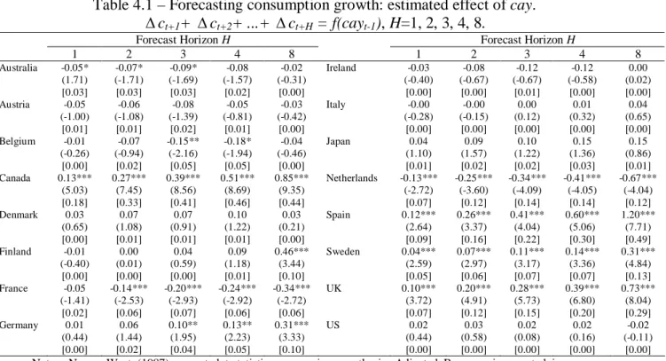
3.3. Forecasting consumption growth
In principle, cay and cday could be a proxy for expected future consumption growth, asset returns, or both. Table 4.1 present the results of the regressions of consumption growth over horizons spanning 1 to 8 quarters, on the lag of trend deviation cday. Table 4.2 provides a summary of the findings when the lag of cday is used as the explanatory variable. In the estimation of the regressions of consumption growth, the dependent variable is, therefore, the H-period consumption growth rate
Δct+1 + … + Δct+H.
Consistent with the findings of Lettau and Ludvigson (2001), the results shown in Table 4.1 suggest that, in general, cayt has no predictive power for future consumption growth. The individual coefficients are not statistically significant and the adjusted R-square is close to zero. A few exceptions include the cases of Canada, France, Netherlands, Spain, Sweden and the UK, where the trend deviation cayt exhibits some predictive power. Nevertheless, one should note that the coefficients are still very
small in magnitude. As a result, the residuals from the contegrating relationship among consumption, asset wealth and labour income can be generally described as a good predictor of asset returns (and not of future consumption growth).
Table 4.1 – Forecasting consumption growth: estimated effect of cay. ct+1+ ct+2+ ...+ ct+H = f(cayt-1), H=1, 2, 3, 4, 8.
Forecast Horizon H Forecast Horizon H
1 2 3 4 8 1 2 3 4 8 Australia -0.05* (1.71) [0.03] -0.07* (-1.71) [0.03] -0.09* (-1.69) [0.03] -0.08 (-1.57) [0.02] -0.02 (-0.31) [0.00] Ireland -0.03 (-0.40) [0.00] -0.08 (-0.67) [0.00] -0.12 (-0.67) [0.01] -0.12 (-0.58) [0.00] 0.00 (0.02) [0.00] Austria -0.05 (-1.00) [0.01] -0.06 (-1.08) [0.01] -0.08 (-1.39) [0.02] -0.05 (-0.81) [0.01] -0.03 (-0.42) [0.00] Italy -0.00 (-0.28) [0.00] -0.00 (-0.15) [0.00] 0.00 (0.12) [0.00] 0.01 (0.32) [0.00] 0.04 (0.65) [0.00] Belgium -0.01 (-0.26) [0.00] -0.07 (-0.94) [0.02] -0.15** (-2.16) [0.05] -0.18* (-1.94) [0.05] -0.04 (-0.46) [0.00] Japan 0.04 (1.10) [0.01] 0.09 (1.57) [0.02] 0.10 (1.22) [0.02] 0.15 (1.36) [0.03] 0.15 (0.86) [0.01] Canada 0.13*** (5.03) [0.18] 0.27*** (7.45) [0.33] 0.39*** (8.56) [0.41] 0.51*** (8.69) [0.46] 0.85*** (9.35) [0.44] Netherlands -0.13*** (-2.72) [0.07] -0.25*** (-3.60) [0.12] -0.34*** (-4.09) [0.14] -0.41*** (-4.05) [0.14] -0.67*** (-4.04) [0.12] Denmark 0.03 (0.65) [0.00] 0.07 (1.08) [0.01] 0.07 (0.91) [0.01] 0.10 (1.22) [0.01] 0.03 (0.21) [0.00] Spain 0.12*** (2.64) [0.09] 0.26*** (3.37) [0.16] 0.41*** (4.04) [0.22] 0.60*** (5.06) [0.30] 1.20*** (7.71) [0.49] Finland -0.01 (-0.40) [0.00] 0.00 (0.01) [0.00] 0.04 (0.59) [0.00] 0.09 (1.18) [0.01] 0.46*** (3.44) [0.10] Sweden 0.04*** (2.59) [0.05] 0.07*** (2.97) [0.06] 0.11*** (3.17) [0.07] 0.14*** (3.36) [0.07] 0.31*** (4.84) [0.13] France -0.05 (-1.41) [0.02] -0.14*** (-2.53) [0.06] -0.20*** (-2.93) [0.07] -0.24*** (-2.92) [0.06] -0.34*** (-2.72) [0.06] UK 0.10*** (3.72) [0.07] 0.20*** (4.91) [0.12] 0.28*** (5.73) [0.15] 0.39*** (6.80) [0.20] 0.73*** (8.04) [0.29] Germany 0.01 (0.44) [0.00] 0.06 (1.44) [0.02] 0.10** (1.95) [0.04] 0.13** (2.23) [0.05] 0.31*** (3.33) [0.10] US 0.02 (0.44) [0.00] 0.03 (0.58) [0.00] 0.02 (0.08) [0.00] 0.02 (0.16) [0.00] -0.02 (-0.11) [0.00]
Notes: Newey-West (1987) corrected t-statistics appear in parenthesis. Adjusted R-square is reported in square brackets.
*, **, *** denote statistical significance at the 10, 5, and 1% level, respectively.
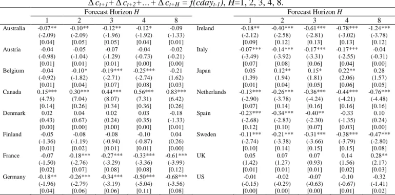
In contrast, Table 4.2 shows that cdayt contains some relevant information about future consumption growth. The coefficients associated with the deviations of consumption from its trend relationship with financial wealth, housing wealth, and labour income are statistically significant for Canada, France, Germany, Ireland, Italy, Netherlands and Sweden. In the case of Canada, this is also reflected in a relatively large adjusted R-square. These findings may be related with the fact that cdayt tracks changes in the composition of asset wealth and, in particular, in housing wealth. Given that housing wealth changes tend to have small but also very persistent effects on consumption,12 cdayt may, therefore, be capturing time-variation in expected returns
and in consumption growth. Finally, one should emphasize that despite this, the
coefficients associated with cdayt in the regressions of consumption growth are quite
12
See Sousa (2010d) for a review of the topic and, in particular, an application of the wealth effects on consumption to the euro area as a whole. Similarly, Sousa (2009) finds evidence of important wealth effects from monetary policy.
small, which is in contrast with the findings in the regressions of real stock returns and real government bond yields. Consequently, cdayt mainly forecasts asset returns.
Table 4.2 – Forecasting consumption growth: estimated effect of cday. ct+1+ct+2+…+ct+H = f(cdayt-1), H=1, 2, 3, 4, 8.
Forecast Horizon H Forecast Horizon H
1 2 3 4 8 1 2 3 4 8 Australia -0.07** (-2.09) [0.04] -0.10** (-2.09) [0.05] -0.12** (-1.96) [0.05] -0.12* (-1.92) [0.04] -0.09 (-1.33) [0.01] Ireland -0.18** (-2.12) [0.09] -0.40*** (-2.58) [0.12] -0.61*** (-2.81) [0.13] -0.78*** (-3.02) [0.13] -1.24*** (-3.78) [0.12] Austria -0.04 (-0.98) [0.01] -0.05 (-1.04) [0.01] -0.07 (-1.29) [0.01] -0.04 (-0.73) [0.00] -0.02 (-0.21) [0.00] Italy -0.07*** (-3.49) [0.07] -0.14*** (-3.92) [0.08] -0.17*** (-3.31) [0.06] -0.17*** (-2.55) [0.04] -0.04 (-0.31) [0.00] Belgium -0.04 (-0.92) [0.01] -0.10* (-1.82) [0.04] -0.19*** (-2.71) [0.07] -0.25*** (-2.74) [0.08] -0.21 (1.62) [0.03] Japan 0.05 (1.39) [0.01] 0.12** (1.94) [0.04] 0.15* (1.81) [0.05] 0.22** (2.06) [0.06] 0.28 (1.57) [0.05] Canada 0.15*** (4.75) [0.14] 0.30*** (7.04) [0.26] 0.44*** (8.07) [0.34] 0.56*** (7.31) [0.36] 0.83*** (6.42) [0.26] Netherlands -0.13*** (-2.90) [0.07] -0.26*** (-3.78) [0.14] -0.36*** (-4.24) [0.16] -0.44*** (-4.21) [0.16] -0.76*** (-4.48) [0.16] Denmark 0.02 (0.43) [0.00] 0.04 (0.67) [0.00] 0.02 (0.24) [0.00] 0.03 (0.35) [0.00] -0.18 (-1.33) [0.01] Spain -0.23*** (-2.68) [0.12] -0.34*** (-2.83) [0.10] -0.40** (-2.30) [0.07] -0.33 (-1.35) [0.03] 0.10 (0.24) [0.00] Finland -0.05 (-1.36) [0.01] -0.08 (-1.19) [0.02] -0.08 (-0.94) [0.01] -0.10 (-0.87) [0.01] 0.04 (0.26) [0.00] Sweden -0.11*** (-2.74) [0.10] -0.21*** (-3.38) [0.14] -0.31*** (-3.66) [0.15] -0.38*** (-3.79) [0.15] -0.47*** (-2.80) [0.08] France -0.07 (-1.50) [0.02] -0.18*** (-2.76) [0.07] -0.27*** (-3.29) [0.08] -0.33*** (-3.36) [0.08] -0.61*** (-3.99) [0.12] UK 0.05 (1.42) [0.01] 0.07 (1.27) [0.01] 0.07 (0.93) [0.01] 0.14 (1.56) [0.02] 0.28** (2.17) [0.03] Germany -0.18** (-1.96) [0.04] -0.26*** (-2.79) [0.06] -0.34*** (-3.19) [0.06] -0.50*** (-5.04) [0.11] -0.68*** (-3.56) [0.08] US -0.01 (-0.15) [0.00] -0.02 (-0.29) [0.00] -0.07 (-0.63) [0.00] -0.10 (-0.67) [0.01] -0.32 (-1.41) [0.02]
Notes: Newey-West (1987) corrected t-statistics appear in parenthesis. Adjusted R-square is reported in square brackets.
*, **, *** denote statistical significance at the 10, 5, and 1% level, respectively.
4. Robustness analysis
4.1. Additional control variables
Campbell and Shiller (1988), Fama and French (1988) and Lamont (1998) show that the ratios of price to dividends or earnings or the ratio of dividends to earnings have predictive power for stock returns. More recently, Goyal and Welsh (2003) argue that because the dividend yield follows a random walk it cannot predict stock prices. However, Robertson and Wright (2006) and Boudoukh et al. (2007) mention that a change in tax legislation in the US in 1983 that legalised share buybacks implies an adjustment of the dividend yield for these and similar effects. Consequently, this adjusted statistic is mean reverting and a good predictor of stock returns.
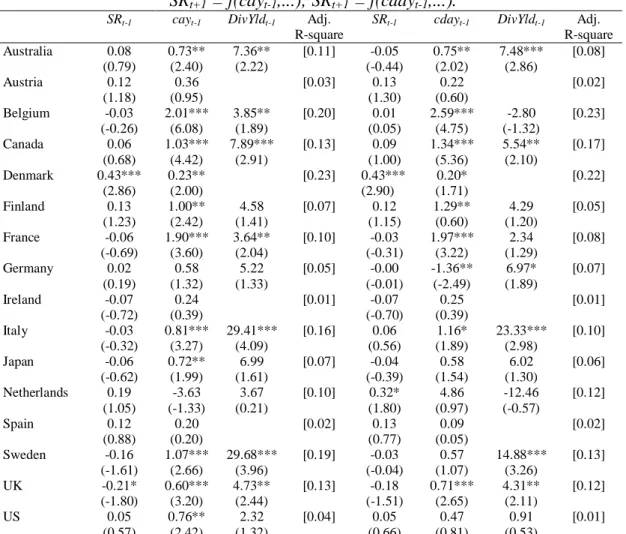
Table 5.1 reports the estimates from forecasting regressions that include additional variables shown to contain predictive power for real stock returns, in particular, the dividend yield ratio (DivYldt). We also add the lag of the real stock returns (SRt-1) as a control variable.
The results show that both the point coefficient estimates of cay and cday and their statistical significance do not change with respect to the findings of Tables 2.1 and
2.2 where only cay and cday were included as explanatory variables. Moreover, the lag of the dependent variable is not statistically significant, a feature that is in accordance with the forward-looking behaviour of stock returns. Finally, the dividend yield ratio (DivYldt) seems to provide relevant information about future asset returns since it is statistically significant in practically all regressions and it improves the adjusted R-square.
Table 5.1 – Forecasting real stock returns: additional control variables.
SRt+1 = f(cayt-1,...); SRt+1 = f(cdayt-1,...). SRt-1 cayt-1 DivYldt-1 Adj.
R-square
SRt-1 cdayt-1 DivYldt-1 Adj.
R-square Australia 0.08 (0.79) 0.73** (2.40) 7.36** (2.22) [0.11] -0.05 (-0.44) 0.75** (2.02) 7.48*** (2.86) [0.08] Austria 0.12 (1.18) 0.36 (0.95) [0.03] 0.13 (1.30) 0.22 (0.60) [0.02] Belgium -0.03 (-0.26) 2.01*** (6.08) 3.85** (1.89) [0.20] 0.01 (0.05) 2.59*** (4.75) -2.80 (-1.32) [0.23] Canada 0.06 (0.68) 1.03*** (4.42) 7.89*** (2.91) [0.13] 0.09 (1.00) 1.34*** (5.36) 5.54** (2.10) [0.17] Denmark 0.43*** (2.86) 0.23** (2.00) [0.23] 0.43*** (2.90) 0.20* (1.71) [0.22] Finland 0.13 (1.23) 1.00** (2.42) 4.58 (1.41) [0.07] 0.12 (1.15) 1.29** (0.60) 4.29 (1.20) [0.05] France -0.06 (-0.69) 1.90*** (3.60) 3.64** (2.04) [0.10] -0.03 (-0.31) 1.97*** (3.22) 2.34 (1.29) [0.08] Germany 0.02 (0.19) 0.58 (1.32) 5.22 (1.33) [0.05] -0.00 (-0.01) -1.36** (-2.49) 6.97* (1.89) [0.07] Ireland -0.07 (-0.72) 0.24 (0.39) [0.01] -0.07 (-0.70) 0.25 (0.39) [0.01] Italy -0.03 (-0.32) 0.81*** (3.27) 29.41*** (4.09) [0.16] 0.06 (0.56) 1.16* (1.89) 23.33*** (2.98) [0.10] Japan -0.06 (-0.62) 0.72** (1.99) 6.99 (1.61) [0.07] -0.04 (-0.39) 0.58 (1.54) 6.02 (1.30) [0.06] Netherlands 0.19 (1.05) -3.63 (-1.33) 3.67 (0.21) [0.10] 0.32* (1.80) 4.86 (0.97) -12.46 (-0.57) [0.12] Spain 0.12 (0.88) 0.20 (0.20) [0.02] 0.13 (0.77) 0.09 (0.05) [0.02] Sweden -0.16 (-1.61) 1.07*** (2.66) 29.68*** (3.96) [0.19] -0.03 (-0.04) 0.57 (1.07) 14.88*** (3.26) [0.13] UK -0.21* (-1.80) 0.60*** (3.20) 4.73** (2.44) [0.13] -0.18 (-1.51) 0.71*** (2.65) 4.31** (2.11) [0.12] US 0.05 (0.57) 0.76** (2.42) 2.32 (1.32) [0.04] 0.05 (0.66) 0.47 (0.81) 0.91 (0.53) [0.01] Notes: Newey-West (1987) corrected t-statistics appear in parenthesis. Adjusted R-square is reported in square brackets. *, **, *** denote statistical significance at the 10, 5, and 1% level, respectively.
On the other hand, Table 5.2 reports the estimates from forecasting regressions that include additional variables shown to contain predictive power for long-term interest rates, in particular, the inflation rate (Inflation) and the deficit-to-GDP ratio (Deficit).
Gale and Orszag (2003) argue that there are two important reasons why government budget deficits may raise nominal interest rates: (i) budget deficits reduce aggregate savings when private savings do not increase by the same amount and there
are no compensating foreign capital inflows; and (ii) budget deficits increase the stock of government debt and, consequently, the outstanding amount of government bonds. In this case, there is a “portfolio effect”, as a higher interest rate on government bonds would be required in order for investors to hold the additional bonds.
Table 5.2 – Forecasting real bond returns: additional control variables.
BRt+1 = f(cayt-1,..); BRt+1 = f(cdayt-1,..). cayt-1 Inflationt-1 Deficitt-1 Adj.
R-square
cdayt-1 Inflationt-1 Deficitt-1 Adj.
R-square Australia 0.60*** (9.45) 0.00*** (3.20) 0.01 (0.20) [0.35] 0.71*** (8.66) 0.00** (2.23) -0.01 (-0.13) [0.35] Austria -0.07 (-1.03) 0.00*** (2.90) [0.11] -0.09 (-1.32) 0.00*** (2.91) [0.12] Belgium -0.41*** (-3.83) -0.00 (-0.25) 0.13*** (7.35) [0.52] 0.15 (1.08) -0.00 (-0.42) 0.13*** (6.61) [0.46] Canada -0.17** (-2.04) 0.00* (1.91) -0.86 (-1.27) [0.10] -0.48*** (-5.92) 0.00 (1.09) -1.26** (-2.13) [0.33] Denmark -0.27** (-2.27) 0.01*** (3.81) [0.17] -0.26** (-2.40) 0.01*** (4.12) [0.17] Finland 0.35** (2.01) -0.00 (-1.50) -0.18 (-1.22) [0.08] 0.59** [2.36] -0.00 (-1.29) -0.11 (-1.06) [0.14] France 0.61*** (5.95) 0.01*** (6.71) 0.01 (0.54) [0.38] 0.87*** (7.59) 0.01*** (7.09) 0.00 (0.03) [0.46] Germany -0.16*** (-4.44) 0.00*** (3.79) 0.07 (0.63) [0.16] -0.09 (-0.96) 0.00** (2.29) -0.12 (-1.31) [0.06] Ireland -0.48*** (-2.96) [0.07] -0.14 (-0.60) [0.01] Italy -0.32*** (-8.47) 0.01*** (6.33) 0.06 (1.45) [0.75] -0.06 (-0.59) 0.02*** (7.37) -0.23*** (-4.40) [0.65] Japan 0.02 (0.05) 0.01*** (4.72) -2.78** (-2.35) [0.36] 0.23 (0.57) 0.01*** (4.73) -3.47** (-2.17) [0.32] Netherlands 0.18** (2.24) 0.00 (1.31) -0.19*** (-3.76) [0.24] 0.36*** (4.01) 0.00 (1.28) -0.14*** (-2.73) [0.30] Spain 0.35** (2.03) 0.02*** (2.74) -0.43** (-2.32) [0.30] 0.25 (0.71) 0.02*** (2.61) -0.39** (-2.00) [0.28] Sweden -0.38*** (-3.15) -0.00 (0.07) -0.18* (-1.81) [0.10] 0.07 (0.29) 0.00 (0.37) -0.10 (-0.89) [0.01] UK -0.18*** (-3.63) 0.00*** (2.51) 0.01 (0.23) [0.18] -0.18** (-2.25) 0.00*** (3.01) -0.07 (-1.37) [0.16] US 0.03 (0.21) 0.01*** (3.79) -0.00 (-0.03) [0.11] 0.16 (1.17) 0.02*** (5.77) -0.66*** (-3.23) [0.34] Notes: Newey-West (1987) corrected t-statistics appear in parenthesis. Adjusted R-square is reported in square brackets.
*, **, *** denote statistical significance at the 10, 5, and 1% level, respectively.
While some studies find that interest rates tend to increase after a rise in the deficit, others do not (Barro and Sala-i-Martin, 1990; Engen and Hubbard, 2004). The empirical findings seem to depend on whether expected or current budget deficits are used as explanatory variables (Upper and Worms, 2003; Laubach, 2009), and also on whether yield differentials in Europe with respect to Germany (Codogno et al., 2003) or interest rate swap spreads are used as the dependent variable (Goodhart and Lemmen, 1999; Afonso and Strauch, 2007).
For Europe, the existing evidence points either to a significant (although small) effect (Bernoth et al., 2003; Codogno et al., 2003; Afonso and Strauch, 2007; Faini,
2006; Afonso and Rault, 2010), or to the absence of impact (Heppke-Falk and Hüfner, 2004). For the US, the effect seems to be substantially larger (Gale and Orszag, 2002). For OECD countries, Barro and Sala-i-Martin (1990) suggest that fiscal variables are unimportant determinants of interest rates, while Ardagna (2009) shows that long-term government bond rates fall in periods of budget consolidation and rise when the fiscal position deteriorates.
Our results corroborate the findings of Tables 3.1 and 3.2. In addition, the lag of the deficit-to-GDP ratio, in general, does not help forecasting bond returns. This is particularly so when the lag of cay is considered in the set of explanatory variables: the lag of the deficit-to-GDP ratio is not statistically significant and its coefficient is small in magnitude. This evidence seems to support the work of Barro and Sala-i-Martin (1990) and, consequently, it highlights the importance of Ricardian equivalence. In contrast, the lag of the inflation rate is statistically significant in roughly all regressions, which suggests that investors use government bonds to hedge against the risk of inflation.
4.2. Nested forecast comparisons
As a final robustness exercise, we make nested forecast comparisons, in which we compare the mean-squared forecasting error from a series of one-quarter-ahead out-of-sample forecasts obtained from a prediction equation that includes either cay or cday as the only forecasting variables, to a variety of forecasting equations that do not include either cay or cday.
We consider two benchmark models: the autoregressive benchmark and the
constant expected returns benchmark. In the autoregressive benchmark, we compare the
mean-squared forecasting error from a regression that includes just the lagged asset return as a predictive variable to the mean-squared error from regressions that include, in addition, cay or cday. In the constant expected returns benchmark, we compare the squared forecasting error from a regression that includes a constant to the mean-squared error from regressions that include, in addition, cay or cday.
A summary of the nested forecast comparisons for the equations of the real stock returns and the government bond yields using respectively cay and cday is provided in Tables 6.1 and 6.2. In general, including cay in the forecasting regressions improves vis-à-vis the benchmark models. This is especially true in the case of the of the constant
expected returns benchmark, supporting the evidence that reports time-variation in
In addition, the models that include cday generally have a lower mean-squared forecasting error. Moreover, the ratios are smaller that the ones presented in Table 6.1, reflecting the better predicting ability for stock returns and government bond yields of
cday relative to cay.
Table 6.1 – One-quarter ahead forecasts of returns: a comparison with benchmark models. cay model vs. constant/AR models.
Real stock returns Real bond returns
MSEcay/MSEconstant MSEcay/MSEAR MSEcay/MSEconstant MSEcay/MSEAR
Australia 0.975 0.984 0.837 0.995 Austria 1.001 1.006 1.003 1.002 Belgium 0.956 0.942 0.955 0.990 Canada 0.990 0.987 0.892 1.038 Denmark 0.971 0.993 0.968 1.003 Finland 0.991 0.998 0.974 1.003 France 0.980 0.997 0.995 0.990 Germany 1.064 1.069 0.973 1.030 Ireland 1.010 1.008 0.964 0.976 Italy 1.001 1.002 0.662 1.001 Japan 0.878 0.877 0.745 0.815 Netherlands 0.995 0.996 0.952 1.002 Spain 0.976 0.984 0.965 0.539 Sweden 1.005 1.005 0.973 1.006 UK 0.997 1.003 1.018 1.047 US 0.991 0.990 0.984 1.006
Notes: MSE represents the mean-squared forecasting error.
*, **, *** denotes statistical significance at the 10, 5, and 1%percent level, respectively.
Table 6.2 – One-quarter ahead forecasts of returns: a comparison with benchmark models. cday model vs. constant/AR models.
Real stock returns Real bond returns
MSEcday/MSEconstant MSEcday/MSEAR MSEcday/MSEconstant MSEcday/MSEAR
Australia 0.981 0.990 0.825 0.997 Austria 1.005 1.008 0.999 1.002 Belgium 0.916 0.924 0.965 0.992 Canada 0.960 0.957 0.889 1.035 Denmark 0.973 0.996 0.974 1.005 Finland 0.997 1.001 0.944 1.004 France 0.981 0.997 0.955 0.989 Germany 1.037 1.041 1.034 1.030 Ireland 1.010 1.010 0.998 0.978 Italy 0.999 1.001 1.006 1.003 Japan 0.879 0.874 0.746 0.797 Netherlands 0.993 0.994 0.890 1.000 Spain 0.977 0.986 0.965 0.553 Sweden 0.991 0.990 1.005 1.006 UK 1.012 1.024 1.021 1.044 US 0.959 0.985 1.039 1.088
Notes: MSE represents the mean-squared forecasting error.
*, **, *** denotes statistical significance at the 10, 5, and 1% level, respectively.
5. Conclusion
This paper uses the representative consumer’s budget constraint to derive an equilibrium relation between the trend deviations among consumption, (dis)aggregate wealth and labour income (summarized by the variables cay and cday) and expected