DOI: 10.22564/rbgf.v37i4.2020
ANALYSIS OF OCEAN TIDE LOADING
ESTIMATED FROM THE GPS COORDINATE TIME SERIES:
A CASE STUDY FOR THE BELÉM, BRASÍLIA, EUSÉBIO, MANAUS
AND SANTA MARIA STATIONS, BRAZIL
Giuliano Sant’Anna Marotta
1, Mário Alexandre de Abreu
1, Ana Cristina Oliveira Cancoro de Matos
2,
João Francisco Galera Monico
3and George Sand Leão Araújo de França
1ABSTRACT.The Earth suffers deformations due to the gravitational attraction of the celestial bodies and the redistribution of water mass occurring by the action of the ocean tide. These effects are known as solid Earth tide (SET) and ocean tide loading (OTL), and can be estimated by observations of the amplitudes and phases of their tidal wave constituents. Considering hat Global Navigation Satellite System (GNSS) observations may be used to estimate these effects and that the solid Earth tide displacement is well resolved, this work estimated and analyzed the amplitudes and phases of the 11 principal constituents of ocean tide loading, using Global Positioning System (GPS) observations. The methodology was applied to data collected from five stations in Brazil, and the amplitudes and phases of the tidal constituents were estimated and evaluated regarding their values and convergence times. The results showed that most of the estimated parameters converged during the analyzed period. In addition, after correcting the effects of ocean tide loading in each GPS solution, using the computed parameters and the existing models, the coordinates were compared and the results presented some local differences, allowing to recommend the use of GPS to estimate tidal constituents considering the local behavior of the point.
Keywords: OTL, tidal constituents, GNSS stations.
RESUMO.A Terra sofre deformações devido à atração gravitacional de corpos celestes e também em função da redistribuição de massa d’água que ocorre por ação da maré oceânica. Estes fenômenos são denominados maré terrestre e carga oceânica, e podem ser estimados por meio das amplitudes e fases das componentes de onda de maré. Considerando que as observações GNSS (Global Navigation Satellite System) podem ser usadas na estimativa destes efeitos e que os deslocamentos devido à maré terrestre são teoricamente bem resolvidos, este trabalho estimou e analisou as amplitudes e fases das 11 componentes principais de carga oceânica, utilizando observações GPS (Global Positioning System). A metodologia foi aplicada a dados coletados em cinco estações instaladas no Brasil, e as amplitudes e fases para as componentes de maré foram estimadas e avaliadas, considerando seus valores e tempo de convergência. Os resultados mostraram que a maioria dos parâmetros estimados convergiu durante o período analisado. Além disso, após corrigir os efeitos de carga oceânica em cada solução GPS, utilizando os parâmetros calculados e os modelos existentes, as coordenadas corrigidas foram comparadas e os resultados apresentaram diferenças locais, permitindo recomendar o uso do GPS na estimativa de componentes de maré considerando o comportamento local do ponto.
Palavras-chave: OTL, componentes de maré, estações GNSS.
Corresponding author: George Sand Leão Araújo de França
1Universidade de Brasília, Observatório sismológico, Campus Universitário Darcy Ribeiro, SG13, Asa Norte, 70910-900, Brasília, DF, Brazil –- E-mails: [email protected], [email protected], [email protected]
2Centro de Estudos de Geodesia, Rua Cotoxó, 611, Conj. 75, Perdizes, 05021-000, São Paulo, SP, Brazil –- E-mail: [email protected]
3Universidade Estadual Júlio de Mesquita Filho, Faculdade de Ciências e Tecnologia, Departamento de Cartografia, Centro Educacional, Rua Roberto Simonsen, 305, 19060-900, Presidente Prudente, SP, Brazil – E-mail: [email protected]
INTRODUCTION
The gravitational attraction of the celestial bodies and the redistribution of water mass resulting from the ocean tide action causes the Earth to undergo deformations (Baker, 1984; Agnew, 2007). These phenomena are known as solid Earth tide (SET) and ocean tide loading (OTL), respectively, and can be described by the amplitudes and phases of the tidal constituents.
For most geophysical and geodetic observations, the displacements caused by SET and OTL must be removed to achieve accurate results. Penna et al. (2007) and Fu et al. (2012) showed that correction models should be as rigorous as possible to avoid spurious effects.
The aforementioned phenomena are conventionally observed and measured using superconducting gravimeters, however, the advance of geodetic observation techniques allowed using the Very Long Baseline Interferometry (VLBI), as demonstrated by Petrov & Ma (2003) and Krásná et al. (2012), and the Global Navigation Satellite Systems (GNSS), as shown in the works of Khan & Tscherning (2001), Allinson et al. (2004), Ito et al. (2009), Yuan (2009) and Alihan et al. (2017) to estimate the displacements caused by the SET and OTL. Yuan et al. (2010) concluded that the GNSS has advantages over the other two methods since, in addition to being low cost, its global coverage enables continuous observations and performing operations in real time as well. In Brazil, Monico et al. (1997) conducted the first study using GPS and the SET, showing the importance of correcting for this effect when high accuracy is desirable.
Penna et al. (2015) reported that the GNSS is being used to estimate tidal displacements since the 2000s, aiming at validating models for correcting for the SET and predicting OTL displacement, considering different OTL models. In regions where these models are imprecise, the OTL displacement estimated by the GNSS can be used to replace the predictions generated by a global model.
Some studies using GPS have been conducted to investigate the OTL models. Among them, Khan & Tscherning (2001), King et al. (2005), Vergnolle et al. (2008), Ito et al. (2009), Yeh et al. (2011), Martens et al. (2016) and Wei et al. (2019) stand out for analyzing the differences between the estimated values and those predicted by the theoretical OTL models. Schenewerk et al. (2001) estimated the vertical tidal displacements for the eight principal diurnal and semidiurnal tidal constituents and found systematic differences between the observed values and those predicted by the analyzed model. Yuan et al. (2009) used GPS data to evaluate the accuracy of
tidal displacement estimates and showed that the measurement error inherent to GPS is not a limiting factor for estimating SET and OTL displacements. Ito & Simons (2011), based on OTL displacements obtained from GPS observations, made inferences about the structure of the asthenosphere. Afterward, Yuan & Chao (2012), also using GPS observations, demonstrated the accuracy of the tide displacement estimates, noting that the errors do not come only from the OTL models, but also from the earth tidal models, which fail to consider the heterogeneities of the interior of the Earth. More recently, Tu et al. (2017) used 8 years’ worth of data from GNSS stations to develop a more accurate method for estimating OTL displacement parameters. In addition, Zhao et al. (2018), using the same data, presented a new method in which global predictions of ocean topology are defined as a priori information to accelerate convergence and improve the accuracy of GPS-estimated displacement parameters.
Considering the studies cited above on the estimation of parameters of SET and OTL using GPS, and considering that the SET is theoretically well resolved, this research focused on estimating and analyzing the local behavior of the amplitudes and phases of the 11 principal tidal constituents (Ssa, Mm, Mf, Q1, O1,
P1, K1, N2, M2, S2, and K2) of the OTL, using the data obtained by
5 GPS stations distributed in the Brazilian territory.
GNSS STATION DATA
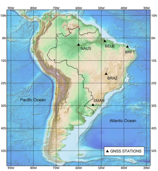
To estimating and analyzing the amplitudes and phases of the tidal constituents, this study used five GNSS stations located within the Brazilian territory, which were selected according to pre-determined criteria, such as: good monument stability; good operation history; good spatial distribution aiming to cover the entire Brazilian territory; and cover a wide range of distances from the coast to allow analyzing the OTL displacement as a function of the distance from the ocean. Additionally, a minimum operational period of 9 years was required to allow covering the complete cycle of most astronomical arguments.
The five GNSS stations (Table 1 and Fig. 1) chosen for the study are located in Belém/PA (BELE), Brasília/DF (BRAZ), Eusébio/CE (BRFT), Manaus/AM (NAUS), and Santa Maria/RS (SMAR). These five stations are part of the Brazilian Network for Continuous Monitoring of GNSS Systems (Rede Brasileira de Monitoramento Contínuo, RBMC) and the SIRGAS-CON (Geocentric Reference System for the Americas - Continuous Monitoring) network, and their daily data are available free of charge on the website of the Brazilian Institute of Geography and Statistics (IBGE, 2018).
Table 1 – Data on the stations used for determining the tidal constituents of SET and OTL.
Station Latitude Longitude Data (Julian day / year) Institutions
Start End
BELE -1.408778 -48.462528 001/2004 246/2018 CENSIPAM (Belém/PA)
BRAZ -15.947472 -47.877861 002/2002 265/2018 IBGE (Brasília/DF)
BRFT -03.877444 -38.425528 001/2006 071/2018 INPE (Eusébio/CE)
NAUS -03.022917 -60.055000 001/2006 147/2018 CENSIPAM (Manaus/AM)
SMAR -29.718917 -53.716583 001/2003 265/2018 UFSM (Santa Maria/RS)
Currently, the stations BELE, BRAZ, BRFT, NAUS and SMAR are equipped with high performance receivers and antennas. These stations had some equipment changed along the period of the data series of this work. However, problems caused by the equipment changing were not identified in the data used.
The obtained GNSS data have a sampling rate of 15 seconds (≈ 0.067 Hz) per record, except for BRFT, which has a 30-second rate (≈ 0.033 Hz), all in RINEX format (Receiver Independent Exchange Format).
OTL CONSTITUENTS
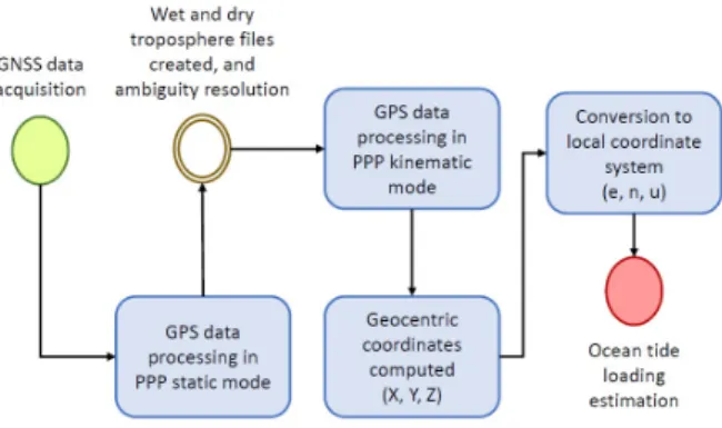
The steps for treating and processing the data used to estimate the tidal constituents for the OTL using data (coordinate time series) from the GNSS positioning technique are shown in Figure 2.
Figure 2 – Flowchart showing the steps for data processing used to estimate the
tidal constituents of OTL.
GNSS PROCESSING
For the purpose of this study, the GNSS data processing (Fig. 2) for estimating the positions and constructing the time series was performed using the Precise Point Positioning (PPP) method of Zumberge et al. (1997). Additionally, all GNSS data processing aiming at improving the precision of the estimated coordinates is performed in two steps. The first consists of processing in static mode (Monico, 2008), so that the ambiguities and estimated tropospheric correction parameters (wet and dry) are solved, among others. The second step consists of kinematic mode processing (King, 2006; Monico, 2008; Yuan et al., 2010; and Martens et al., 2016), using the ambiguities already solved and the tropospheric correction models estimated in the first step, to obtain a better positioning accuracy.
The GNSS data processing is similar to that presented by Thomas et al. (2007), King et al. (2005) and Allinson et al. (2004). The daily observation files for each station were
processed using the GNSS-Inferred Positioning System and Orbit Analysis Simulation Software (GIPSY/OASIS), version 6.4, to obtain the coordinates in the geocentric cartesian system. As GIPSY/OASIS version 6.4 processes only GPS data, the GLONASS, Galileo and Beidou observations were discarded in this work. Also non-fiducial orbits was used which, according to Blewitt et al. (1992), are free of errors related to the reference system employed.
Table 2 presents the parameter settings and models used to estimate the GPS coordinates in kinematic mode.
Two different processing strategies in the kinematic mode were performed for each of the stations. The first processing used all the corrections presented in Table 2, while the second processing did not use the OTL correction. This strategies allowed to compare the results of the data processing, after estimating the OTL constituents and using them in the processed data.
At the end of the processing, the velocity vector values from each of the analyzed stations were estimated and applied to the coordinates in the geocentric cartesian system, so that all the calculated coordinates are referred to the same time, allowing to compare the positional variation over the time series. Subsequently, the geocentric Cartesian coordinates (X, Y, Z) were transformed into coordinates in the local geodetic system (e, n, u).
To generate the time series, the first calculated coordinate was used as a reference and subtracted from all subsequent coordinates. This procedure allowed to observe only the positional variation over time. Also, the time series were edited to eliminate gross errors so that they could be used to estimate the amplitudes and phases of the tidal constituents. This edition consisted of eliminating points that exceeded the standard deviation value of the time series at 99.7% confidence level (3σ). Estimation of the OTL constituents
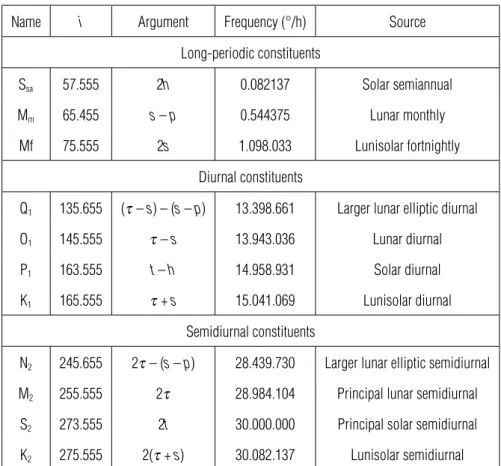
After the the GPS data processing, 11 principal tidal constituents (Table 3) were estimated (Fig. 2) and analysed. Of these constituents, according to Yuan (2009), four diurnal (Q1, O1, P1,
and K1) and four semidiurnal (N2, M2, S2, and K2) are responsible
for 98% (depending of the geographical position) of the entire tidal signal.
According Doodson (1921) and Foreman & Henry (1989) all tidal frequencies are linear combinations of six astronomical arguments, being: mean lunar time (τ), mean longitude of the
Moon (s), mean longitude of the Sun (h), longitude of the Moon’s mean perigee (p), negative of the longitude of the Moon’s mean ascending node on the ecliptic (n’), and longitude of the Sun’s
Table 2 – Parameters and models used for GPS processing (ITRF, 2008; Petit & Luzum, 2010; IBGE, 2018).
Processing Interval 300 seconds
2nd order Ionosphere correction Global Ionosphere Maps (GIM) / IONEX (Ionosphere Exchange)
Troposphere mapping function Vienna Mapping Function (VMF)
Orbit, clock and antenna phase center corrections Non-fiducial JPL (Jet Propulsion Laboratory) products
Antenna phase center igs08_www.atx
Ambiguity WLPB (Wide-lane and Phase bias) products/JPL
Ocean tide load correction FES2014
SET correction IERS 2010
Reference frame ITRF2008 (IGb08 orbits)
Table 3 – Principal tidal constituents (Source: Adapted from Melchior, 1983). i is the Doodson number, t is the mean
solar time,τis the mean lunar time, s is the mean longitude of the Moon, p is the longitude of the Moon’s mean
perigee and h mean longitude of the Sun.
Name i Argument Frequency (°/h) Source
Long-periodic constituents
Ssa 57.555 2h 0.082137 Solar semiannual
Mm 65.455 s – p 0.544375 Lunar monthly
Mf 75.555 2s 1.098.033 Lunisolar fortnightly
Diurnal constituents
Q1 135.655 (τ– s) – (s – p) 13.398.661 Larger lunar elliptic diurnal
O1 145.555 τ– s 13.943.036 Lunar diurnal
P1 163.555 t – h 14.958.931 Solar diurnal
K1 165.555 τ+ s 15.041.069 Lunisolar diurnal
Semidiurnal constituents
N2 245.655 2τ– (s – p) 28.439.730 Larger lunar elliptic semidiurnal
M2 255.555 2τ 28.984.104 Principal lunar semidiurnal
S2 273.555 2t 30.000.000 Principal solar semidiurnal
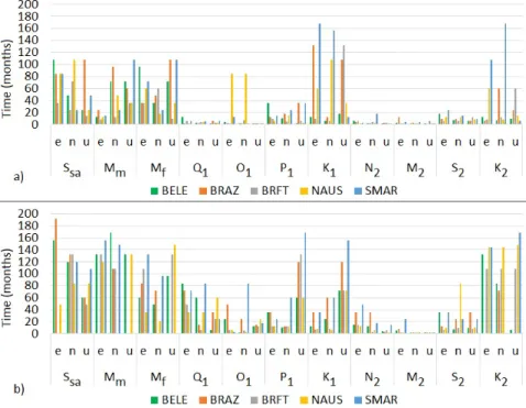
Figure 3 – Time of stabilization, in months, of the OTL amplitudes (a) and phases (b) values for BELE, BRAZ, BRFT,
NAUS, and SMAR stations.
mean perigee (p’). The approximate periods for each of these 6 variables are 24.84 hours, 27 days, 1 year, 8.8 years, 18.6 years and 21,000 years.
In general, the harmonic analysis requires calculating the amplitudes and phases for a finite number of sinusoidal functions with known frequencies. Therefore, the displacement due to tide x(t) can be estimated as presented by Yuan et al. (2010):
x(t) =
max(k)
∑
k=1
fkAkcos [ωkt+χk(t0) + uk−ϕk] (1)
where Ak,ϕk andωk are the amplitudes, phases and angular
frequence of the tidal constituent at the station, respectively; fk
and uk are used to account for the modulating effects with
the 18.6-year period of the lunar node;χk is the astronomical
argument at reference time t0; and k represents each tidal
constituent.
In this study, the T_TIDE - Tidal Analysis Toolbox, version 1.4b (updated on 2019) was used to estimate the principal constituents of the OTL for the GNSS stations (Fig. 1 and Table 1). All procedures applied and theoretical description of the Toolbox used in this study are presented by Pawlowicz et al. (2002).
The tidal constituents were estimated using different time interval of the time series data, starting with one month and
ending with all of the time series data available for each station. The chosen processing mode allowed to follow the time of stabilization of amplitude and phase values over the analyzed historical series.
The amplitudes and phases were estimated for the OTL constituents. Consequently, to compute and analyze the tidal constituents, GPS solutions with and without OTL correction were generated.
TIDAL ANALYSIS
The time of stabilization of the OTL amplitudes and phases values estimated of the 11 principal constituents are presented in Figure 3 and Table 4.
In general, Figure 3 and Table 4 shows that all Long-periodic (Ssa, Mmand Mf) and some Diurnal (O1, P1and
K1) and Semidiurnal (K2) constituents either did not converge or
converged only after a long time of observation.
The Ssa constituents converged between the 15th and the
196th month, with only two occurrences of non-convergence. The amplitudes of the Mmand Mfconstituents converged between
the 12th and the 180th month, while the convergence of phases occurred between the 21st and 168th month, but 8 phases did not converge (Table 4).
Table 4 – Time of stabilization, in months, of the amplitudes (A) and phases (F) values of the 11 principal OTL
constituents from the BELE, BRAZ, BRFT, NAUS, and SMAR stations, in e, n and u components. NS means not stabilized.
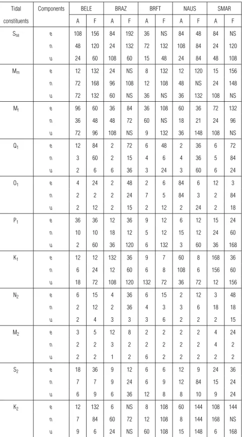
Tidal Components BELE BRAZ BRFT NAUS SMAR
constituents A F A F A F A F A F Ssa e 108 156 84 192 36 NS 84 48 84 NS n 48 120 24 132 72 132 108 84 24 120 u 24 60 108 60 15 48 24 84 48 108 Mm e 12 132 24 NS 8 132 12 120 15 156 n 72 168 96 108 12 108 48 NS 24 148 u 72 132 60 NS 36 NS 36 132 108 NS Mf e 96 60 36 84 36 108 60 36 72 132 n 36 48 48 72 60 NS 18 21 24 96 u 72 96 108 NS 9 132 36 148 108 NS Q1 e 12 84 2 72 6 48 2 36 6 72 n 3 60 2 15 4 6 4 36 5 84 u 2 6 6 36 3 24 3 60 6 24 O1 e 4 24 2 48 2 6 84 6 12 3 n 2 2 2 24 7 5 84 3 2 84 u 2 12 2 15 2 12 2 24 2 18 P1 e 36 36 12 36 9 12 6 12 15 24 n 10 10 18 12 5 12 15 12 24 60 u 2 60 36 120 6 132 3 60 36 168 K1 e 12 12 132 36 9 7 60 8 168 36 n 6 24 12 60 6 8 108 6 156 60 u 18 72 108 120 132 72 36 72 12 156 N2 e 6 15 4 36 6 15 2 12 3 48 n 2 12 2 36 4 3 3 6 18 18 u 2 4 3 3 3 6 2 2 2 15 M2 e 3 5 12 8 2 2 2 2 4 24 n 2 2 3 2 2 2 2 2 4 2 u 2 2 1 2 6 2 2 2 2 2 S2 e 18 36 9 12 6 6 12 9 24 36 n 7 7 9 24 6 9 12 84 15 24 u 6 9 6 36 12 8 8 10 9 24 K2 e 12 132 6 NS 8 108 60 144 108 144 n 7 84 60 72 12 108 8 144 168 NS u 9 6 24 NS 60 108 15 148 6 168
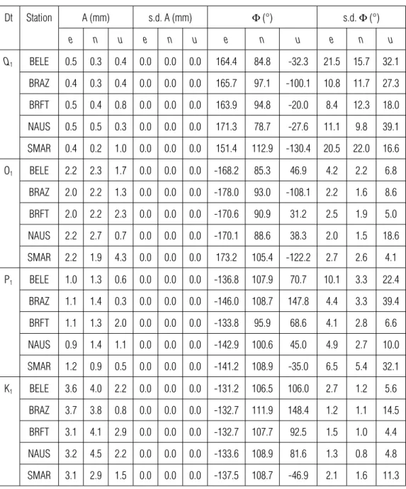
Table 5 – OTL amplitudes (A) and phases (F) estimated for three principal tidal constituents (long-periodic tides - Lpt) from the BELE, BRAZ, BRFT,
NAUS and SMAR stations.
Lpt Station A (mm) s.d. A (mm) Φ (°) s.d. Φ (°) e n u e n u e n u e n u Ssa BELE 0.6 0.7 4.2 1.0 1.0 1.0 -72.2 -64.9 86.6 46.3 50.2 20.1 BRAZ 0.8 0.9 8.5 0.0 1.0 2.0 -51.8 -67.6 56.2 28.8 39.0 10.9 BRFT 0.3 1.5 4.8 0.0 1.0 1.0 -80.8 -32.6 66.5 105.3 30.1 16.4 NAUS 1.0 1.2 9.4 0.0 1.0 2.0 -13.5 -37.9 45.8 19.1 39.8 9.2 SMAR 0.7 1.0 1.6 0.0 1.0 3.0 -54.2 -69.5 -168.3 31.9 35.7 114.9 Mm BELE 0.1 0.2 0.5 0.0 0.0 1.0 -24.9 155.9 -164.5 167.7 173.4 141.1 BRAZ 0.0 0.4 0.3 0.0 1.0 1.0 -0.7 158.4 -77.2 260.5 102.9 202.5 BRFT 0.2 0.3 0.7 0.0 1.0 1.0 17.4 164.0 120.6 134.7 131.9 124.3 NAUS 0.3 0.2 0.7 0.0 0.0 1.0 30.2 140.4 23.4 78.3 173.1 126.8 SMAR 0.3 0.4 0.3 0.0 1.0 2.0 26.3 135.0 151.6 66.0 103.4 224.1 Mf BELE 0.4 0.4 1.0 1.0 1.0 1.0 112.0 159.1 169.9 82.7 90.2 85.1 BRAZ 0.3 0.7 0.1 0.0 1.0 1.0 110.6 176.8 123.7 84.1 51.8 242.5 BRFT 0.2 0.6 0.7 0.0 1.0 1.0 81.1 151.7 166.4 142.7 83.1 106.1 NAUS 0.4 0.6 0.5 0.0 1.0 1.0 96.8 170.3 159.4 59.1 80.1 146.2 SMAR 0.3 0.7 0.8 0.0 1.0 2.0 121.6 168.9 87.2 74.8 56.3 189.0
For the diurnal components, all amplitudes and phases converged between the 2nd and 168th month (Table 4). However, the K1 component presents the worst convergence results in
general.
The analysis of the semidiurnal components show that many amplitudes and phases converged in the 2nd month, requiring a maximum of 168 months for convergence (Table 4). The worst convergence results were observed for K2and, for all 11
constituents analyzed, M2required the shortest time to converge,
in general, compared to the others.
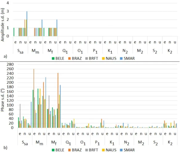
The OTL amplitudes and phases values for the analyzed stations are presented in Tables 5, 6 and 7. The uncertainty values are also shown in Figure 4.
The results shown in Tables 5, 6 and 7 indicate greater displacement in the vertical coordinates (u) compared to the horizontal coordinates (e and n). This occurs because the Earth deformation has a greater effect on the altimetric component than on the planimetric one.
Analyzing separately the constituents M2 and S2, which
presented the largest amplitudes, it is possible to verify that the largest displacement due to OTL occurs at the BRFT station, which is approximately 6 km away from the Atlantic Ocean. The BELE station located approximately 130 km from the Atlantic Ocean has the 2nd largest displacement. The BRAZ and NAUS stations have very close values, and both are about 1000 km distant from the Atlantic Ocean. Further, the SMAR station did not follow the pattern observed in the other stations since it had the smallest
Table 6 – OTL amplitudes (A) and phases (F) estimated for four principal tidal constituents (diurnal tides - Dt) of OTL from the BELE, BRAZ,
BRFT, NAUS and SMAR stations.
Dt Station A (mm) s.d. A (mm) Φ (°) s.d. Φ (°) e n u e n u e n u e n u Q1 BELE 0.5 0.3 0.4 0.0 0.0 0.0 164.4 84.8 -32.3 21.5 15.7 32.1 BRAZ 0.4 0.3 0.4 0.0 0.0 0.0 165.7 97.1 -100.1 10.8 11.7 27.3 BRFT 0.5 0.4 0.8 0.0 0.0 0.0 163.9 94.8 -20.0 8.4 12.3 18.0 NAUS 0.5 0.5 0.3 0.0 0.0 0.0 171.3 78.7 -27.6 11.1 9.8 39.1 SMAR 0.4 0.2 1.0 0.0 0.0 0.0 151.4 112.9 -130.4 20.5 22.0 16.6 O1 BELE 2.2 2.3 1.7 0.0 0.0 0.0 -168.2 85.3 46.9 4.2 2.2 6.8 BRAZ 2.0 2.2 1.3 0.0 0.0 0.0 -178.0 93.0 -108.1 2.2 1.6 8.6 BRFT 2.0 2.2 2.3 0.0 0.0 0.0 -170.6 90.9 31.2 2.5 1.9 5.0 NAUS 2.2 2.7 0.7 0.0 0.0 0.0 -170.1 88.6 38.3 2.0 1.5 18.6 SMAR 2.2 1.9 4.3 0.0 0.0 0.0 173.2 105.4 -122.2 2.7 2.6 4.1 P1 BELE 1.0 1.3 0.6 0.0 0.0 0.0 -136.8 107.9 70.7 10.1 3.3 22.4 BRAZ 1.1 1.4 0.3 0.0 0.0 0.0 -146.0 108.7 147.8 4.4 3.3 39.4 BRFT 1.1 1.3 2.0 0.0 0.0 0.0 -133.8 95.9 68.6 4.1 2.8 6.6 NAUS 0.9 1.4 1.1 0.0 0.0 0.0 -142.9 100.6 45.0 4.9 2.7 10.0 SMAR 1.2 0.9 0.5 0.0 0.0 0.0 -141.2 108.9 -35.0 6.5 5.4 32.1 K1 BELE 3.6 4.0 2.2 0.0 0.0 0.0 -131.2 106.5 106.0 2.7 1.2 5.6 BRAZ 3.7 3.8 0.8 0.0 0.0 0.0 -132.7 111.9 148.4 1.2 1.1 14.5 BRFT 3.1 4.1 2.9 0.0 0.0 0.0 -132.7 107.7 92.5 1.5 1.0 4.4 NAUS 3.2 4.5 2.2 0.0 0.0 0.0 -133.6 108.9 81.6 1.3 0.8 4.8 SMAR 3.1 2.9 1.5 0.0 0.0 0.0 -137.5 108.7 -46.9 2.1 1.6 11.3
displacement caused by OTL. At this case, although located about 350 km from the Atlantic Ocean, SMAR is located further to the south and, according to Lyard et al. (2006), it is adjacent to a region with relatively small ocean-tide amplitudes.
Also in relation to the results shown in Tables 5, 6 and 7 and Figure 4, it is possible to verify that the largest uncertainties are
associated with the constituents that had the longest convergence time (Fig. 3 and Table 4). In this case, it may be suggested that: the long-periodic tide constituents have influence of non-tidal quasi-periodic effects; K1 and K2 may be associated with the
satellite orbit error and multipath effect, because the period of the K1coincides with that of the satellite constellation and the
Table 7 – OTL amplitudes (A) and phases (F) estimated for four principal tidal constituents (semidiurnal tides - Sdt) of OTL from the BELE,
BRAZ, BRFT, NAUS and SMAR stations.
Sdt Station A (mm) s.d. A (mm) Φ (°) s.d. Φ (°) e n u e n u e n u e n u N2 BELE 1.0 1.0 4.2 0.0 0.0 0.0 -141.4 -119.1 46.7 7.4 4.7 2.3 BRAZ 0.4 0.8 2.5 0.0 0.0 0.0 -167.4 -156.7 44.1 9.7 4.5 3.6 BRFT 0.9 1.6 7.2 0.0 0.0 0.0 -173.8 -148.4 25.3 4.5 2.1 1.6 NAUS 0.4 0.5 2.3 0.0 0.0 0.0 -176.6 -145.4 52.4 8.8 6.6 3.5 SMAR 0.4 0.7 1.8 0.0 0.0 0.0 -150.5 -178.0 72.2 22.0 17.4 6.8 M2 BELE 4.6 4.7 19.1 0.0 0.0 0.0 -135.5 -97.5 60.1 1.4 0.8 0.5 BRAZ 2.4 3.9 10.6 0.0 0.0 0.0 -169.6 -135.1 45.1 1.8 1.0 0.8 BRFT 4.2 7.2 33.5 0.0 0.0 0.0 -165.1 -127.7 38.1 0.9 0.4 0.3 NAUS 2.1 2.7 9.8 0.0 0.0 0.0 -171.9 -119.8 63.8 1.7 1.4 0.8 SMAR 1.7 3.4 6.5 0.0 0.0 0.0 -162.7 -159.6 64.8 6.0 3.4 1.9 S2 BELE 1.5 1.9 7.9 0.0 0.0 0.0 -114.4 -53.4 144.1 4.3 2.2 1.3 BRAZ 1.5 1.4 4.9 0.0 0.0 0.0 -143.5 -90.2 148.1 3.0 2.7 1.7 BRFT 1.9 2.3 8.9 0.0 0.0 0.0 -142.3 -96.5 104.9 2.2 1.5 1.3 NAUS 1.1 0.8 5.3 0.0 0.0 0.0 -134.0 -75.1 145.3 3.5 4.4 1.3 SMAR 1.0 1.5 2.2 0.0 0.0 0.0 -135.6 -112.4 131.5 8.4 7.6 4.9 K2 BELE 0.4 0.4 1.3 0.0 0.0 0.0 -76.4 -52.4 100.9 17.6 9.7 8.2 BRAZ 0.1 0.6 0.3 0.0 0.0 0.0 -26.7 -82.4 157.0 32.4 6.1 31.3 BRFT 0.2 0.9 3.1 0.0 0.0 0.0 -164.7 -76.1 64.6 16.8 4.3 3.7 NAUS 0.2 0.2 0.6 0.0 0.0 0.0 -116.7 -93.6 13.5 22.1 22.3 15.8 SMAR 0.9 1.4 0.6 0.0 0.0 0.0 -40.0 -104.8 -94.4 9.4 7.8 19.3
period of the K2is almost the same as the satellite orbital period
(Wei et al., 2019); and, according to Wei et al. (2019), P1may be
disturbed by residual GPS signal propagation errors or non-tidal daily cycles in the atmosphere because its period is very close to solar day.
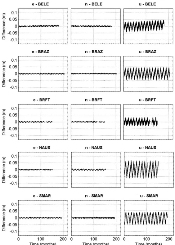
Figure 5 shows the differences found between the PPP time series signal corrected using the OTL displacements estimated in
this work, subtracted from the corrected PPP time series signal using the theoretical oceanic loading model.
Figure 5 shows that the difference signal presents less dispersion in e and n components due to the diminished influence of the OTL effect on the planimetric components. The difference signal for u component of the 5 analyzed stations shows a sinusoidal behavior of largest amplitude. These diferences may
Figure 4 – Uncertainty (standard deviations - s.d.) values of estimated OTL amplitudes (a) and phases (b) for BELE, BRAZ, BRFT, NAUS, and
SMAR stations.
be related especially to the phase difference between one or more tidal constituents. However, the greatest differences characterized by long-period signal (Figure 5) are related to the hydrological load effect that has not been corrected in the GPS data processing.
CONCLUSION
This paper presents a methodology for estimating the amplitudes and phases of the 11 principal tidal constituents of OTL using GPS positioning data. The obtained results allowed to reach a few conclusions and present some recommendations.
The differences given by the subtraction between the signals corrected using the estmated OTL displacements and the theoretical models for u component showed a sinusoidal behavior. This behavior may be related to the phase difference between one or more tidal constituents used. One possibility to try to eliminate this phase difference would be to correct for the hydrological and atmospheric load effects on the GPS
data processing, or in the time series. It is likely that after correcting for these effects, the resulting signal should become less noisy allowing to determine amplitudes and phases with less uncertainty. However, these two effects are very dynamic and, therefore, difficult to model with the required precision. Another option would be to analyze the place of each station monument to identify the factors causing greater uncertainty to the observed signal.
It was expected that the convergences of the diurnal and semidiurnal constituents would require less time, but this delay may be related to the period of the time series. The used series began at a time when the GPS constellation was formed by 24 satellites only, causing periods throughout the day with a somewhat unfavorable geometry of satellites so that the determined satellite position became less precise. Later, as the number of satellites of the GPS constellation increased, the problems regarding geometry were greatly minimized.
Figure 5 – Differences between the PPP time series signal corrected using the OTL displacements estimated in this work subtracted from the corrected PPP time series
The M2 tidal constituent, responsible for the greatest
contribution to tidal displacements, required a short time for the amplitudes and phases to converge (Tables 4 and 5), demonstrating that this constituent was determined with good precision.
The analysis of the M2and S2constituents in u component,
which had the greatest amplitude, shows that the behavior of OTL displacements is consistent with reality, since the stations closest to the equator presented the highest amplitudes, whereas the stations at higher latitudes presented the smaller amplitudes. This occurs because the tidal force is higher in the region near the Equator, becoming weaker towards the Poles.
The OTL displacements were also consistent since the BRFT station, the closest to the Atlantic Ocean presented the highest values for the M2 and S2 constituents in u component. These
values also decreased as the distance between the analyzed station and the ocean increased. However, although the SMAR station is near to the Atlantic Ocean, the smallest displacements can be associated with its location further south and, according to Lyard et al. (2006), adjacent to a region with relatively small ocean-tide amplitudes.
ACKNOWLEDGEMENT
The authors thank IBGE for providing GNSS data, and CNPq (460443/2014-3), INCT-ET (465613/2014-4) and CPRM for financial support.
REFERENCES
AGNEW DC. 2007. Earth Tides. Treatise on Geophysics and Geodesy. In: HERRING TA (Ed.). Treatise on Geophysics. New York: Elsevier, v. 3, p. 163-195.
ALIHAN NSA, WIJAYA DD, DIN AHM, BRAMANTO B, OMAR AH, PRADHAN B. 2017. Spatiotemporal Variations of Earth Tidal Displacement over Peninsular Malaysia Based on GPS Observations. In: PRADHAN B (Ed.). GCEC 2017. Lecture Notes in Civil Engineering. Springer, Singapore, 9: 809-823. doi: 10.1007/978-981-10-8016-6_59. ALLINSON CR, CLARKE PJ, EDWARDS SJ, KING MA, BAKER TF, CRUDDACE PR. 2004. Stability of direct GPS estimates of ocean tide loading. Geophysical Research Letters, 31(L15603), pp. 1-4.
BAKER TF. 1984. Tidal deformations of the Earth. Science Progress, 69: 197-233.
BLEWITT G, HEFLIN MB, WEBB FH, LINDQWISTER UJ, MALLA R. 1992. Global coordinates with centimeter accuracy in the international terrestrial reference frame using GPS. Geophysical Research Letters, 19: 853-856.
DOODSON AT. 1921. The harmonic development of the tide-generating potential. Proceedings of the Royal Society of London, Series A, 100: 305-329.
FOREMAN MGG, HENRY MF. 1989. The harmonic analysis of tidal model time series. Adv. Water Resources, 12: 109-120.
FU Y, FREYMUELLER JT, Van DAM T. 2012. The effect of using inconsistent ocean tidal loading models on GPS coordinate solutions. Journal of Geodesy, 86(6): 409-421.
IBGE. 2018. RBMC - Rede Brasileira de Monitoramento Contínuo dos Sistemas GNSS. Available on: < http://www.ibge.gov.br/home/ geociencias/geodesia/rbmc/rbmc.shtm?c=71>. Access on: September 23, 2018.
ITO T, SIMONS M. 2011. Probing asthenospheric density, temperature, and elastic moduli below the western United States. Science, 332(6032): 947-951.
ITO T, OKUBO M, SAGIYA T. 2009. High resolution mapping of Earth tide response based on GPS data in Japan. Journal of Geodynamics, 48(3-5): 253-259.
ITR.. 2008. International Terrestrial Reference Frame. Available on: < http://itrf.ensg.ign.fr/ITRF_solutions/2008/ITRF2008.php> Access on: September 23, 2018.
KHAN SA, TSCHERNING CC. 2001. Determination of semi-diurnal ocean tide loading constituents using GPS in Alaska. Geophysical Research Letters, 28(11): 2249-2252.
KING MA. 2006. Kinematic and static GPS techniques for estimating tidal displacements with application to Antarctica. Journal of Geodynamics, 41(1-3): 77-86.
KING MA, PENNA NT, CLARKE PJ, KING EC. 2005. Validation of ocean tide models around Antarctica using onshore GPS and gravity data. Journal of Geophysical Research, 110(B08401): 1-21.
KRÁSNÁ H, NÉE S, BÖHM J, BÖHM S, SCHUH H. 2012. SET parameters from VLBI measurements and FCN analysis. In: International VLBI Service for Geodesy & Astrometry General Meeting. Madrid, Spain, 4-9 March 2012: 405-409.
LYARD F, LEFÈVRE F, LETELLIER T, FRANCIS O. 2006. Modelling the global ocean tides: a modern insight from FES2004. Ocean Dynamics, 56: 394-415.
MARTENS HR, SIMONS M, OWEN S, RIVERA L. 2016. Observations of ocean tidal load response in South America from subdaily GPS positions. Geophysical Journal International, 205: 1637-1664.
MELCHIOR P. 1983. The tides of the planet Earth. 2nd ed., Brussels: Oxford, Pergamon Press, 653 pp.
MONICO JFG. 2008. Posicionamento pelo NAVSTAR-GPS: descrição, fundamentos e aplicações. 2nd ed., São Paulo, Brazil: UNESP Press, 480 pp.
MONICO JFG, ASHKENAZI V, MOORE T. 1997. High precision GPS network with precise ephemerides and Earth body tide model. Revista Brasileira de Geofísica, 15(2): 155-160.
PAWLOWICZ R, BEARDSLEY B & LENTZ S. 2002. Classical tidal harmonic analysis including error estimates in MATLAB using T_TIDE. Computers and Geosciences, 28: 929-937.
PENNA NT, CLARKE PJ, BOS MS, BAKER TF. 2015. Ocean tide loading displacements in western Europe: 1. Validation of kinematic GPS estimates. Journal of Geophysical Research: Solid Earth, 120(9): 6523-6539.
PENNA NT, KING MA, STEWART MP. 2007. GPS height time series: short-period origins of spurious long-period signals. Journal of Geophysical Research Solid Earth, 112(B2): 1074-1086.
PETIT G & LUZUM B. 2010. IERS Conventions, IERS Technical Note 36. Frankfurt am Main: Verlag des Bundesamts für Kartographie und Geodäsie. 179 pp. ISBN 3-89888-989-6.
PETROV L & MA C. 2003. Study of harmonic site position variations determined by very long baseline interferometry. Journal of Geophysical Research: Solid Earth, 108(B4): 2190.
SCHENEWERK MJ, MARSHALL J, DILLINGER W. 2001. Vertical ocean-loading deformation derived from the global GPS network. Journal of the Geodetic Society of Japan, 47(1): 237-242.
THOMAS ID, KING MA, CLARKE PJ. 2007. A comparison of GPS, VLBI and model estimates of ocean tide loading displacements. Journal of Geodesy, 81(5): 359-368.
TU R, ZHAO H, ZHANG P, LIU J, XIAOCHUN L. 2017. Improved method for estimating the ocean tide loading displacement parameters by GNSS precise point positioning and harmonic analysis. Journal of Surveying Engineering, 143(4): 040170051-040170059.
VERGNOLLE M, BOUIN M-N, MOREL L, MASSON F, DURAND S, NICOLAS J, MELACHROINOS SA. 2008. GPS estimates of ocean tide
loading in NW-France: Determination of ocean tide loading constituents and comparison with a recent ocean tide model. Geophysical Journal International, 173(2): 444-458.
WEI G, WANG Q, PENG W. 2019. Accurate Evaluation of Vertical Tidal Displacement Determined by GPS Kinematic Precise Point Positioning: A Case Study of Hong Kong. Sensors, 19(2559): 1-14.
YEH TK, HWANG C, HUANG JF, CHAO BF, CHANG MH. 2011. Vertical displacement due to ocean tidal loading around Taiwan based on GPS observations. Terrestrial Atmospheric and Oceanic Science, 22(4): 373-382.
YUAN L. 2009. Determination of tidal displacements using the Global Positioning System. Doctoral thesis. Department of Land Surveying & Geo-Informatics, The Hong Kong Polytechnic University, 203 pp. YUAN L & CHAO BF. 2012. Analysis of tidal signals in surface displacement measured by a dense continuous GPS array. Earth and Planetary Science Letters, 355-356: 255-261. https://www. sciencedirect.com/science/journal/0012821X/355/supp/C
YUAN LG, DING XL, ZHONG P, CHEN W, HUANG DF. 2009. Estimates of ocean tide loading displacements and its impact on position time series in Hong Kong using a dense continuous GPS network. Journal of Geodesy, 83(11): 999-1015.
YUAN LG, DING XL, SUN HP, ZHONG P, CHEN W. 2010. Determination of ocean tide loading displacements in Hong Kong using GPS technique. Science China, 53(7): 993-1007.
ZHAO H, ZHANG Q, TU R, LIU Z. 2018. Determination of ocean tide loading displacement by GPS PPP with priori information constraint of NAO99b global ocean tide model. Marine Geodesy, 41(2): 159-176. ZUMBERGE JF, HEFLIN MB, JEFFERSON DC, WATKINS MM, WEBB FH. 1997. Precise point positioning for the efficient and robust analysis of GPS data from large networks. Journal of Geophysical Research, 102(B3): 5005-5017.
Recebido em 5 de dezembro de 2019 / Aceito em 10 de fevereiro de 2020 Received on December 5, 2019 / Accepted on February 10, 2020