Alan R.R. de Freitas

Aggregation Trees for visualization and dimension reduction in

many-objective optimization

Alan R.R. de Freitas

_{, Peter J. Fleming}

_{, Frederico G. Guimarães}

c_{Department of Electrical Engineering, Federal University of Minas Gerais, Av. Antônio Carlos 6627, 31270-901 Belo Horizonte, MG, Brazil}

a r t i c l e

i n f o

Article history: Received 10 March 2014

Received in revised form 25 November 2014 Accepted 28 November 2014

Available online 5 December 2014

Keywords: Aggregation Trees Multi-objective optimization Many-objective optimization Visualization

Evolutionary computation Polar graphs

a b s t r a c t

This paper introduces the concept of Aggregation Trees for the visualization of the results of high-dimensional multi-objective optimization problems, or many-objective problems and as a means of performing dimension reduction. The high dimensionality of many-objective optimization makes it difficult to represent the relationship between many-objectives and solutions in such problems and most approaches in the literature are based on the rep-resentation of solutions in lower dimensions. The method of Aggregation Trees proposed here is based on an iterative aggregation of objectives that are represented in a tree. The location of conflict is also calculated and represented on the tree. Thus, the tree can repre-sent which objectives and groups of objectives are the most harmonic, what sort of conflict is present between groups of objectives, and which aggregations would be helpful in order to reduce the problem dimension.

Ó2014 Elsevier Inc. All rights reserved.

1. Introduction

Real-world optimization problems often have many conflicting objectives and, as a consequence, multi-objective optimi-zation problems have become a major field of research. Sometimes these problems can be solved by aggregating all of the objectives into a single objective function that gives some weight to each of the objectives. However, very often, it is more important to understand the relationship between the objectives in order to make decisions with a reasonable understand-ing of the trade-off involved among the possible choices.

When there are few objectives to be considered, evolutionary algorithms are usually suitable to find the best combination of solutions to a problem and it is not very difficult to represent that set of possibilities (Section2). As the number of objec-tives grow, we reach the field of many-objective problems (Section2.3). The optimization of these problems becomes more challenging as most solutions become incomparable as the Pareto dominance selection becomes less discriminating. That means that any solution in our set of candidates is almost always better than all other solutions for at least one specific com-bination of objective weights. Besides, representing quality for a set of solutions in this context is equally a problem.

In order to address this problem, we propose the concept of Aggregation Trees (Section3). Aggregation Trees iteratively group objective functions in tree nodes according to their harmony (a concept mathematically defined in Section4), similar

http://dx.doi.org/10.1016/j.ins.2014.11.044 0020-0255/Ó2014 Elsevier Inc. All rights reserved.

⇑ Corresponding author.

E-mail addresses:alandefreitas@iceb.ufop.br(A.R.R. de Freitas),p.fleming@sheffield.ac.uk(P.J. Fleming),fredericoguimaraes@ufmg.br(F.G. Guimarães). URL:http://www.alandefreitas.com(A.R.R. de Freitas).

Information Sciences

to an agglomerative hierarchical clustering method. Thus, it represents the relationship between conflicting groups of objec-tives for a problem. It also represents the globality or locality of the conflict, the region of concentration of the calculated conflict (as mathematically defined in Section5) through branch colors and it shows which is the best combination of objec-tives to be aggregated for dimension reduction.

The contributions of the proposed approach are:

Visualization of results for many-objective problems including particularly: – The amount of harmony and conflict between relevant groups of objectives. – The globality or locality of the conflict.

– The region where the conflict is more intense in the objective space, when conflict is not equally spread in the objec-tive space.

Representation of the most useful aggregations in order to iteratively perform dimensionality reduction on any number of objectives of the original problem.

Robustness in relation to problems where the relationship between objectives is not linear. This is obtained by employing a non-parametric analysis.

The position of nodes in the tree suggest convenient positions for the representation of absolute objective values in par-allel coordinate plots.

Polynomial computational cost and ease of implementation.

Thus, as the majority of solutions in many-objective problems tend to be non-dominated, Aggregation Trees can be used as a method for providing the decision maker with enough information to restrict the preference area for a problem, restrict the domain of search variables, create new constraints for the problem or reduce the number of objectives in a further analysis.

We describe the algorithm in Section6, analyze the polynomial time complexity of the suggested method in Section6.1, and apply it to test instances in Section7. We then conclude our paper with discussions about the method and suggestions concerning possible future work (Section8).

2. Historical perspective

Complex problems often require the consideration of many criteria of performance, and, as a consequence, multi-objec-tive problems are a well studied topic in the scientific literature. In simple approaches, objecmulti-objec-tives are aggregated into a single objective function that takes into account the utility of each objective. However, in a multi-objective problem, the solution set can be found to represent the trade-off between those objectives[12,10,21]. The solutions that represent this compro-mise are in the Pareto-optimal set, which has only non-comparable optimal solutions in the objective space. This means that no solution in the Pareto-set is preferable to another in relation to all objectives.

2.1. Multi-objective optimization problems

Definition 2.1. A multi-objective optimization problem can be defined as:

minðf1ðxÞ;f2ðxÞ;. . ._;fmðxÞÞ; x2 F ð1Þ

wherexis a solution for the problem andf_iðxÞis thei-th objective function to be minimized.

Each functionfiðxÞmaps the optimization variables of a candidate solutionxto an objective value represented in one dimension of the objective space, i.e.,fiðÞ:Rn#R.

Definition 2.2. The set of all combinations of possible values for optimization variables defines the search spaceS:

S ¼fx¼ fðx1;

v

v

v

where each variablexiassumes the value

v

Definition 2.3. If the problem has constraints, those constraint functionsg_iðxÞ;i¼1;. . .;rdefine the feasible set of solutions

F:

F ¼fx2 S:giðxÞ60;i¼1;. . ._;rg ð3Þ

In multi-objective problems, the comparison between solutions has to consider all objective functions. We can only sayx1 is a better solution thanx2_ifx1_{is better on all the objective functions.}

solutions) which are Pareto-optimal, that is, solutions that cannot be improved in any of the objectives without incurring an inferior result for another objective.

Definition 2.5. A feasible solutionx_{2 F is Pareto optimal iff 9=y2 F such that fðyÞ fðxÞ. Solving a multi-objective} optimization problem involves finding the Pareto setPdenoted as:

P ¼_fx_{2 F: 9=y2 F;fðyÞ fðxÞg ð6Þ}

2.2. Evolutionary multi-objective evolutionary algorithms

Due to their flexibility and inherent set-based strategy, evolutionary algorithms have been widely used for addressing multi-objective problems. The original algorithms for multi-objective problems used Pareto-based ranking to assign fitness to different solutions[10,21]. Many other Evolutionary Algorithms have been proposed since then with good results for multi-objective problems[13,68,34]. Recent algorithms often involve decomposition of the original problem into a set of sin-gle objective subproblems[66,14,39]or make use of auxiliary indicators to evaluate solutions[3].

Besides the flexibility of evolutionary algorithms, these approaches also permit mechanisms for controlling diversity [69,37,34,29,38,26,51,5], integration of the decision-making into the process[20,45,42,64,2], and ease of creation of hybrid approaches[25].

2.3. Many-objective problems

Despite the success of those algorithms for addressing real-world problems, their performance reduces dramatically for problems that have more than three objectives. This fact led to the definition of a new term to better refer to this context, namely, many-objective problems[32]. In those problems, Pareto-based ranking is no longer an effective discriminator and the majority of solutions are non-comparable, thus compromising the convergence of the algorithms.

Besides, there is a memory cost of representing a Pareto set that grows exponentially with the number of conflicting objectives and the visualization of that Pareto set also becomes difficult in many-dimensions, which in turn become a burden for the decision-making process as well.

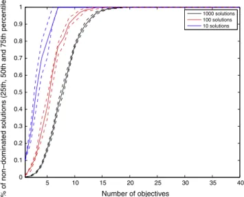
Khare et al.[33]showed the poor scalability of NSGA-II, PESA and SPEA2 in scalable test functions. Hughes[27]showed that aggregation methods with multi-start perform better than MOEAs. Knowles & Corne[35]showed that MOEAs do not perform better than random search in problems with more than 10 objectives. Purshouse & Fleming[48]found that the abil-ity of variation operators to produce solutions that dominate their parents decrease with increasing numbers of objectives. In order to represent this effect,Fig. 1shows the percentage of non-dominated solutions in a set of objective values randomly generated with a Gaussian distribution. Thex-axis is the number of objectives, while they-axis represents the percentage of non-dominated solutions on an initial set of solutions for a problem of that dimension.

5 10 15 20 25 30 35 40

0 0.1 0.2 0.3 0.4 0.5 0.6 0.7 0.8 0.9 1

Number of objectives

% of non−dominated solutions (25th, 50th and 75th percentiles)

1000 solutions 100 solutions 10 solutions

It is easy to verify that the more objectives we have, the higher the percentage of initial solutions that are already non-dominated. When we use a smaller set of solutions, this percentage increase is even faster. Each combination of a number of objectives and set size was tested 100 times and the dotted lines show the 25th and 75th percentiles. These percentiles are always very close to the average values. Usually, if those initial solutions are used in an elitist evolutionary algorithm, all results become non-dominated after a very few generations. Observations like this have been made elsewhere in the liter-ature, see for instance[4].

There is still another way to intuitively see how the number of solutions needed to represent the Pareto-set grows expo-nentially. For a single-objective problem, the solution is represented by a single point. For 2, 3, 4,. . .objectives, the Pareto set may be represented by a curve, a surface, a hyper-surface, and so on. Thus, even if we keep only the extreme solutions for each dimension (which are not generally the most appropriate ones) we would need at least 2M1_{solutions to represent the} trade-offs.

This exponential relationship shows the importance of treating many-objective optimization as a distinct class of problems. Since there are mainly non-dominated solutions in sets of any practical size, understanding the relationship between the objectives and providing the most useful information to decision makers in polynomial time is more fruitful and representative than the non-polynomial task, in space and time, of finding a front with the best solutions.

Alternatives for solving many-objective problems often introduce certain preferences or measures of the decision maker into the optimization process: different dominance relations to improve discrimination at each generation[51,55,5], mod-ifying ranking methods[17,70,52,62,35], other fitness measures involving indicators[67,6,8,9,2,53], or the simultaneous optimization of many scalarized objective functions[28,30,31,63].

2.4. Objective reduction

Another approach to address these problems is dimensionality reduction through identification of redundant objectives [8,9,53,57,22].

Brockhoff and Zitzler[8,9]propose a method of objective reduction geared towards direct integration into the evolution-ary search. Their algorithm depends on a change in the dominance structure. They also present the problem of finding a min-imum objective subset, maintaining the given dominance structure with a given error. A greedy algorithm removes objectives if the dominance relations do not change with the removal of the objective because it is perceived as a non-con-flicting one.

Saxena et al.[53]employ Principal Component Analysis (PCA) of the objective values in order to identify related objec-tives. The PCA is tailored to handle non-linear relations between the objectives and the technique is then embedded into NSGA-II. Other papers have also presented new techniques based on maximum variance unfolding and PCA for nonlinear reduction of objectives[54]. Those techniques remove dependencies in the non-dominated solutions.

Jaimes et al.[40]employ unsupervised feature selection to reduce the number of objectives according to their correlation. Distant objectives are considered as conflicting. In a similar approach to that of Brockhoff and Zitzler[9], the algorithm also seeks the minimum objective subset with minimum error.

Singh et al.[56]present a Pareto Corner Search. This algorithm focuses only on corners among the non-dominated solu-tions. After that, the number of resulting non-dominated solutions from a reduction of the achieved solutions indicates whether the objectives are essential or whether they can be reduced.

Freitas et al.[22]present a mathematical formulation of the concept of harmony previously defined by other articles [47,48,9,24]. The more harmonic two objectives are, the more it indicates that they can be aggregated into a compound objective function without much loss in the representation of the Pareto-set.

2.5. Visualization of results

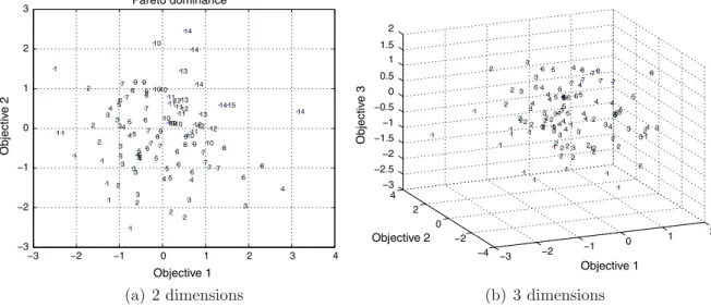
The results of multi-objective problems in 2 dimensions can be easily represented in a simple two-axis Cartesian repre-sentation as inFig. 2(a). In that representation, each solution is displayed as a point. The non-dominated solutions are iden-tified by a number 1 in the first front. Those are the non-comparable, or non-dominated, solutions. All other solutions are worse than at least one solution in the first front, assuming minimization of the objectives. Usually, dominated solutions are not presented in the graph when we want to make the information clearer.

By means of a simple extension,Fig. 2(b) can be used for problems with 3 objectives. In that case, the shape of the non-dominated solutions also has an additional dimension. One can see the reduction in the number of fronts, as also shown in[4].

A problem with the representation method used inFig. 3is that we can only see conflict between adjacent objectives. In order to better represent solutions in high dimensions, other approaches often involve mapping the objectives onto lower dimensions. However, it is not possible to perform any mapping to a lower dimensional space without losing information and general existing methods for such mapping do not tend to take care to preserve the underlying Pareto-dominance rela-tionship between solutions in a higher dimension.

Eddy and Lewis propose cloud visualization[18], in which the designer can view design information as well as the objec-tive space simultaneously.

Obayashi and Sasaki[46]use self-organizing maps to mine the solutions and find trade-offs in the Pareto solutions of 4 dimensions. Furthermore, the authors create a second self-organizing map of cluster-averaged design variables to analyze their roles on the quality of the solutions.

Mattson and Messac[44]used an s-Pareto frontier as the result of a filter applied to the original non-dominated objective values. However, this approach leads to a loss of dimension representation.

Lotov[41]uses a technique of Interactive Decision Maps to represent solutions in the objective space as an alternative to parallel coordinate plots for problems having between three and seven objectives.

Agrawal et al.[1]use a Hyper-space Diagonal Counting method as a visualization tool for multi-objective solutions. Köppen and Yoshida[36]use an approach that aims for the preservation of Pareto-dominance relations in lower dimen-sions. Their algorithm searches for a mapping that has few wrong dominance relations and preserves nearest neighbor rela-tions. Thus, mapping itself is a multi-objective problem which is handled by an evolutionary algorithm.

−3 −2 −1 0 1 2 3 4

−3 −2 −1 0 1 2 8 11 4 7 2 7 6 14 12 10 7 14 9 6 1 11 9 15 1 1 9 1 9 1 10 10 5 7 10 12 3 10 14 4 2 4 5 8 11 3 3 5 2 14 6 10 10 5 7 8 13 6 3 6 13 1 ₁₃ 11 12 8 10 5 4 5 3 1 7 3 9 6 7 5 4 3 11 12 9 2 4 3 2 12 2 7 8 1 8 3 7 5 4 3 2 7 3 4 6 5 Objective 1 Objectiv e 2

(a) 2 dimensions

−3 −2 −1

0 1 2 −4 −2 0 2 4 −3 −2.5 −2 −1.5 −1 −0.5 0 0.5 1 1.5 3 8 4 1 2 3 2 5 3 5 5 1 2 5 5 5 7 2 4 4 1 3 7 8 4 2 2 2 7 1 2 4 4 Objective 1 7 8 5 4 3 6 4 3 2 7 1 6 5 2 1 4 6 5 4 3 6 2 3 2 3 5 4 4 2 5 3 1 3 3 1 5 2 4 4 2 2 3 2 3 6 4 3 5 1 4 2 3 1 3 2 1 3 2 2 2 1 1 2 1 2 1 Objective 2 1 Objectiv e 3

(b) 3 dimensions

Fig. 2.Representation of the quality of many solutions for MOP.

1 2 3 4 5 6 7

min max Objectives Objectiv e v alues

Blasco et al.[7]employ level diagrams forn-dimensional Pareto front analysis. In this technique, each objective is repre-sented on a separate diagram. The method utilizes an ideal point to classify the points.

Mascia and Brunato[43]analyze techniques for visualization of search landscapes in combinatorial optimization. They propose techniques that explicitly render geographic metaphors used by researchers. Adaptations on those algorithms could make them useful for visualizing objective spaces.

Tušar and Filipicˇ[58]describe a methodology for presenting the quality of multi-objective solutions with 4 dimensions. In their method prosections (projections of a section[23]) are used to perform dimension reduction.

Yoshimi et al.[65]present a spherical self-organized map to visualize solutions with many objectives. The spherical approach addresses the issue that similar data differing in few variables are often placed at opposite ends of the map.

Walker et al.[59]conducted an extensive review of methods for Pareto-visualization and presented their own methods. They use spectral seriation to rearrange the solutions and objectives plotted on a heatmap. They also present two methods to visualize solutions in a plane: one that maps a set to the interior of a polygon on a plane, and another that uses a measure of dominance distance between solutions to yield visualizations in two dimensions.

Fieldsend and Everson[19]propose a method to visualize Pareto relationships in two-dimensional scatterplots. They attempt to create a two-dimensional projection with minimal loss of dominance information. In their plot, points represent solutions and connecting lines represent dominance relations.

In a multi-objective problem, there are many features the decision maker will want to see from the data returned by any optimization algorithm. Among those features, it is important to have a visualization method in which it is possible to easily perceive components such as:

1. The amount of conflict between the objectives. 2. The amount of harmony between the objectives. 3. The nature of those features in the set of points. 4. The region where those features appear, if they are local.

This last feature is important for the decision maker because if there is only conflict for solutions which are poor in regard to two given objectives, the decision maker would probably take decisions very different from a case in which the conflict happens only among good solutions.

Besides that, in many-objective optimization, we have interest in also visualizing:

1. A comparison of the conflict between the combinations of objectives.

2. Which combination and reduction of objectives into a simple summary would cause less distortion in the final represen-tation of the Pareto front

3. The conflict we have between groups of objectives, not only pairs of individual objectives

The appropriate answer to these questions would provide useful information for the decision maker to understand the problem and then take the appropriate measures to filter those solutions and restrict the preference area until there is only a single solution. We can see that the accurate measures of those features would involve (i) the robust calculation of conflict and harmony between objectives that are often in different units, (ii) the definition of the cause of the final values to define locality and globality, and (iii) a method of visualization that could contain all this information in a way that is easy to interpret.

3. The concept of an Aggregation Tree

In this paper, we introduce a form of representing the relationship between objectives in a many-objective problem. An aggregation tree is based on the idea that the more harmonious two objectives are, the better suited they are to be reduced or grouped into a single new scalarized objective value[47,48]. With the help of a formalized non-parametric mathematical definition of harmony[22], a tree can show the relationships between conflicting objectives.

In order to exemplify the utility of the proposed Aggregation Trees, consider the set of solutions represented in the par-allel coordinate plot ofFig. 4(a). Every adjacent pair of objectives in this set of 40 solutions contains a distinctive harmony and conflict relationship. Objectives 1, 2, 4, 6, 8, 10, and 12 are in complete harmony because they have the same objective values. A mathematical formulation of conflict and harmony is given in Section4.

Fig. 4(b) represents the relationship between those objectives and their reducibility in the structure of a tree. The objec-tives are iteratively clustered by their amount of harmony while percentages on parent nodes show the conflict between the children objectives. Any parent node represents the aggregation of the children objectives into a new objective. More spe-cifically, this Aggregation Tree has the following properties:

Leaf nodes represent objectives in the formfi, whereiis the objective number.

those objectives, given the measure to be explained in Section4. For example, the nodef10þf80%represents a com-pound objective with objectives 10 and 8. It also shows that there is 0% of conflict between those two objectives, so that they can be grouped because they are in complete harmony.

Other parent nodes represent higher order compound objectives formed in a similar way. The values of conflict in those parents include only the conflict between their direct children’s compound objectives. For instance, besides representing the compound objective formed with objectives 10, 8, 6, and 4, the nodef10þf8þf6þf40%also shows that there is 0% of conflict between the compound objectivesf10þf8andf6þf4. The conflict 0% between even objectives occurs because the objective values of even objectives inFig. 4(a) always return to the same values as in objectivef₂, while the odd objec-tives are being used to didactically employ various possible relationships between objecobjec-tives.

Objectives are respectively grouped according to their harmony and therefore distant cousins in the tree represent less harmonious objectives.

Nodes in black represent global conflict. Values in red represent local conflict more concentrated on good values for those objectives. Values in blue represent conflict for bad solutions in the objectives. Measures of conflict concentration at a region of the objective space are given in Section5.

When two compound objectives are grouped into one new compound objective, the conflict in the previous compound objectives is not considered in the conflict of the new objective. Thus, an optional feature (not included in this example to facilitate visualization) is to have the size of each branch of the tree proportional to its conflict, in order that we can perceive the accumulated conflict from the root node to any position of the tree.

The values of conflict in the tree can also be normalized or rescaled if high values of conflict would make cognition more difficult. This strategy has the benefit of not depending on the measure of conflict being used. However, we lose the absolute values of conflict by making use of this approach. Thus, we cannot infer the general amount of conflict between objectives a problem.

The first advantage of visualizing the relationship between objectives in an Aggregation Tree is that it is straightforward to see the conflict between the objectives and the objectives are grouped according to their harmony. Thus, in a case where the decision maker wishes to make compound objectives according to their harmony and therefore their reducibility, the nodes give information on which would be the best ones to group. Instead of only showing the conflict between every pair of objectives, the tree also shows the conflict between groups of objectives that could be aggregated instead of showing the conflict between many groups of objectives which are not related. Also, the colors represent the globality or locality, and regions of the conflict.

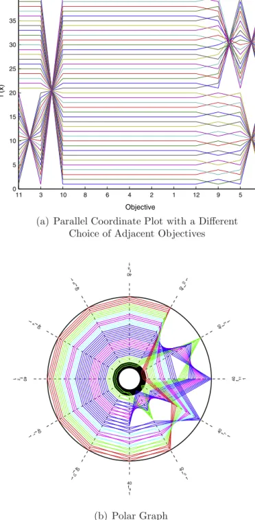
One more useful application of the tree comes from the idea that if two leaf nodes are distant cousins in the tree, there is little harmony between those objectives. Thus, the final position of leaf nodes gives a convenient way to choose good adja-cent objectives in a parallel coordinate plot, such as the one inFig. 5(a). In this Figure, it is easier to identify the relationship between the objectives using their absolute values because harmonious objectives are nearby, not disrupting the represen-tation of conflicting objectives as occurs for each pair of objectives inFig. 4(a).

1 2 3 4 5 6 7 8 9 10 11 12

0 5 10 15 20 25 30

Objective

f (x)

Given the usefulness of this ordering of the objectives and the fact that we might also want to visualize the two most distant cousins on the tree, we propose the use of an improved representation of the absolute values in a Polar Graph, such as the one inFig. 5(b). Similarly to parallel coordinate plots, each line in the Polar Graph represents a solution and the main difference between them is that the Polar Graph has a toroidal structure that allows the representation of extreme objectives in the parallel coordinate plot, which, according to the tree, must be of interest because the nodes representing those objec-tives are the furthest cousins possible. Also, the interior of the circle represents inferior values (high values for minimization objectives) for each of the objectives while the most external part represents better values in that objective. The values are linearly normalized and the range of absolute values in each objective is represented outside the circle. A clustering tech-nique, PSA[49]in this example, is also applied here to facilitate visualization of the results.

Thus, in our example, the toroidal structure of the Polar Graph is capable of showing the conflicting relationship between objectives 11 and 7. Also, as close cousins in the tree represent objectives in harmony, it is possible to visualize the effect of each jump from one branch of the tree to the other. For instance, it is easy to visualize that solutions in green, in general, have high values in the harmonious objectivesf10;f8;f6;f4;f2;f1;f12;f1, andf9. We can see that those good values in the harmo-nious objectives are compensated with low values forf3and medium values forf11andf5. Yet, low values in the harmonious objectives for solutions in red are generally compensated by high values inf11andf3.

One last interesting use of the data provided by this analysis of conflict is the direct first-order conflict between each of the original objectives, such as the one inTable 1. The table represents the conflict between every pair of objectives, accord-ing to the metric to be presented in Section4.

Thus, an Aggregation Tree is a tool to help decision makers compute and visualize redundancy and conflict between objectives. Its main applications are grouping objectives for dimensionality reduction and visualization of the analyses using trees and polar graphs. The MATLAB source code for all these algorithms is available fromhttp://www.alandefreitas.com/. Sections4 and 5describe the mathematical formulation of conflict, harmony, and conflict region. In Section6we describe in detail the algorithm for constructing a Aggregation Tree; its time complexity is described in Section6.1.

4. Conflict and harmony as a form of aggregation

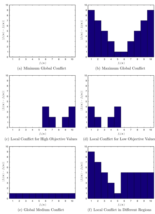
Fig. 6represents many kinds of conflict and harmony in parallel coordinate plots of two objectives. We say there is con-flict[47,48,9,24]between two objectives when good values for one of them imply bad values for another. On the other hand, we say there is harmony between two objectives when improvement in the first objective leads to improvement in the sec-ond. We can see from the Figure how not only the amount of conflict varies but the conflict can also be concentrated in a certain region of the objective space.

Thus, the concept of conflict may depend on what the user expects as ‘‘good’’ and ‘‘bad’’ values for each of the objectives. Our perception of conflict also depends on the shape of the Pareto front formed by the best solutions because it might be that the range of values known for each objective is very large due to outliers, thereby changing our perception of conflict.

However, the concept of harmony only implies that improvement in one objective leads to improvement in another. In this sense, harmony may not always be the exact opposite of conflict. Harmonious objectives are presented in a parallel coor-dinate plots by non-crossing lines. Thus, it has to do with the possibility of joining the objectives through summation with-out loss of quality in the Pareto front. If we want to group two objectives into a new compound objective, it is best to group those objectives with greater harmony even if there is perception of some level of conflict between them.

According to these loose definitions, we propose[22]specific mathematical formulations of conflict and harmony by specifying three general types of conflict: direct, max–min, and non-parametric conflict. Harmony, on the other hand is inversely proportional to non-parametric conflict.

Table 2shows the mathematical formulation of those three kinds of conflict.Cabrepresents the conflict between objec-tivesaandb.cminandcmaxrepresent the minimum and maximum values possible of conflict for that measure.Xijis the value of the solutioni(of a total ofnsolutions) on objectivej. Also,Rijis the rank ofXijwithinX:j. If there are ties in the calculation ofRij, we break the ties by using the rank that causes least conflict with the other objective being compared.

Each formulation is built on a different view of what can be considered conflict between two objectives. These different views translate into different forms of normalizing objectives. The measure of harmony is a mathematical formulation of the idea that crossing lines in parallel coordinate plots represent a lack of harmony. The 3rd and 4th columns contain the minimum and maximum values of conflict that can be obtained in that metric. This is helpful for normalizing the results, if required.

A non-parametric measure of conflict works without the assumption of comparability between objectives. As this metric reflects the degree by which lines would be crossing between objectivesaandbin a parallel coordinate plot, it can also be used to formulate the measure of harmony defined in Eq.(7). This measure of harmony returns values that range between 0 to 1.

Hab¼1Cab

cmax ð7Þ

11 3 10 8 6 4 2 1 12 9 5 7

0 5 10 15 20 25 30

Objective

f (x)

(a) Parallel Coordinate Plot with a Different

Choice of Adjacent Objectives

40 f11 1 40 f

3 1

40 f

10

1 40

f 8 1

40

f

6 1

40f

4

1

40

f

2

1

40 f

1

1

40 f 12 1

40

f₉

1

40 f5

1

40 f7

1

(b) Polar Graph

It is important to mention that, if we invert the solution qualities for the dimensions, the calculation ofCabis equivalent to Spearman’s footrule[16]and it is similar to Spearman’s Rho[11]in the sense that it is a nonparametric measure of statistical dependence between two variables. As mentioned already, the more harmonious two objectives are, the better candidates they are to be grouped into a new compound objective, and this fact is conveniently used by the Aggregation Trees to rep-resent the relationship between objectives.

5. Conflict concentration regions

Since non-parametric conflict and harmony are measured as the summation of rank differences, the location of those dif-ferences is also generally relevant information. It is important for the decision maker to know whether the conflict is occur-ring for the best or worst values for the objectives being compared. That information is relevant because if the conflict only occurs for solutions with poor objective values on those objectives, that means that the conflict would not exist if those were the only objectives being considered.

For instance,Fig. 6presents many examples of trade-offs between two objectives in a parallel coordinate plot and all the results are shown in terms of ranks. InFig. 6(a), an improvement in objective 1 always leads to an improvement in objective 2. In this case, there is no conflict between the objectives and the behavior is global. This is the best case for which to make a new compound objective. If there is little non-parametric conflict and much harmony, most of the behavior will still be global because the harmony is global. InFig. 6(b), the behavior is also global because there is con-flict everywhere. This is the extreme case of concon-flict, where an improvement in one objective necessarily causes dete-rioration in another.

Fig. 6(c) and (d), on the other hand, are examples in which the conflict is only local. In the first case ofFig. 6(c), conflict only occurs for solutions which are poor in relation to those objectives, considering a minimization problem. In those cases, the removal of other objectives would eventually cause the trade-off to disappear, as for only the objectives being analyzed, only one solution would be in the Pareto front. InFig. 6(d), however, the elimination of other objectives could not lead to less conflict between the objectives being considered because five solutions would still be in the first front because the conflict between those objectives is inherent. That demonstrates the importance of representing not only the globality of conflict but also its region.

Having less than maximum conflict does not necessarily mean that conflict is local. The example inFig. 6(e) shows a case of global medium conflict. Another special case is the one represented inFig. 6(e) in which there is local conflict but the region of conflict is different for the objectives. In that case, there would be a Pareto front even if just those two objectives are taken into consideration, because the conflict is located around good solutions for objective 1. In that case, the conflict is located in the good values for objective 1 and bad values for objective 2.

Since harmony is expressed in terms of the accumulated difference of ranks in the solutions, it is then important to see where those differences come from and whether those differences are more located around good or bad solutions.Fig. 7 shows the difference of values for the same examples inFig. 6. Thexaxis has the rank of each solution in objective 1 while theyaxis has the absolute difference to the corresponding solution in objective 2. We could also use this sort of plot for objective 2 in thexaxis with different results because, as the example inFig. 6(e) has shown, we can have the same conflict located in different regions of different objectives.

In the first case ofFig. 7(a), there is no difference at all between any of the solutions because there is no conflict. In the opposite case of maximum conflict,Fig. 7(b) shows how the globality of conflict leads to a symmetric difference of values. Also we can see that in the case of maximum conflict it does not mean that there will be high values of difference everywhere because median solutions have less conflict.

Fig. 7(c) and (d) show cases of conflict which are specifically local, that is, concentrated on one particular region of the objective space. In those cases, the differences are respectively concentrated on the worst and best values. Symmetrical dif-ference value graphs reflect on a smaller scale the graph ofFig. 7(b) because even though conflict is local, it is locally the

Table 1

Conflict between the objectives in the solutions ofFig. 4(a). The values range from 0 (minimum conflict) to 1 (maximum conflict).

1 2 3 4 5 6 7 8 9 10 11 12

1 0 1 0 .25 0 .25 0 .05 0 1 0

2 0 1 0 .25 0 .25 0 .05 0 1 0

3 1 1 1 1 1 1 1 1 1 .25 1

4 0 0 1 .25 0 .25 0 .05 0 1 0

5 .25 .25 1 .25 .25 .5000 .25 .275 .25 1 .25

6 0 0 1 0 .25 .25 0 .05 0 1 0

7 .25 .25 1 .25 .5 .25 .25 .275 .25 1 .25

8 0 0 1 0 .25 0 .25 .05 0 1 0

9 .05 .05 1 .05 .275 .05 .275 .05 .05 1 .05

10 0 0 1 0 .25 0 .25 0 .05 1 0

11 1 1 .25 1 1 1 1 1 1 1 1

1 2 1

2 3 4 5 6 7 8

(a) Minimum Global

Non-Parametric Conflict

1 2

1 2 3 4 5 6 7 8

(b) Maximum Global

Non-Parametric Conflict

1 2

1 2 3 4 5 6 7 8 9 10

(c) Local Non-Parametric Conflict

for High Objective Values

1 2

1 2 3 4 5 6 7 8 9 10

(d) Local Non-Parametric Conflict

for Low Objective Values

1 2

1 2 3 4 5 6 7 8 9 10

(e) Global Medium

Non-Parametric Conflict

1 2

1 2 3 4 5 6 7 8 9 10

(f) Local Non-Parametric Conflict in

Different Locations in Each Objective

same behavior of maximum conflict. These two graphs illustrate how the distribution of the differences is concentrated in certain areas if the conflict is local.

Fig. 7(c) is a case of global conflict again. Similarly to the first two cases, the distribution of the differences is spread around the values on the right. However, the area is smaller than inFig. 7(b) because there is less conflict. The last case ofFig. 7(f) is conflict located in a different region for the two objectives. In relation to objective 1, the conflict is for low rank solutions and the values of difference have formed areas of similar value because even though the lines for high rank values are parallel, there is a large difference in ranks for the group and, therefore, conflict for this whole set of solutions. However, what indicates the concentration of conflict in a certain region is that the area is more concentrated in low rank values for the first solutions, that is, solutions 1, 2, 3, 4, and 5. For the second half, the area is then spread on those high rank solutions, indicating the lower the solution’s rank, the more conflict there is.

From graphs such as the one presented, we have then to identify whether the values of conflict are coming from low or high values. In order to do that, letRijrepresent the rank of the solutionxion objectivefjðxÞ. LetR0ijbe these rank values linearly scaled from1 to 1 for objectivefjðxÞ. The values ofR0ijnow represent the weight of that solution for low (-1) or high (+1) rank solutions.

Each differencejRiaRibjbetween ranks (as it is used by the non-parametric measure of conflict presented in Section4) is multiplied by its weightR0

iain order that we can infer whether those values are concentrated on high or low values. Positive values indicate concentration on high values and negative values indicate low values. This summation is then divided by Lða;bÞmaxin order that we can have aLða;bÞvalue that ranges from1 to +1. Thus, the following measure of conflict region Lða;bÞof objectiveain relation to objectivebis used for the Aggregation Trees:

Lða;bÞ ¼

Pn

i¼1jRiaRibjR

0 ia

Lða;bÞmax ð8Þ

Lða;bÞmaxis the maximum value ofLða;bÞ, which is described by the following equation:

Lða;bÞmax¼ X

n

i¼bn=2cþ1

j2i b3n=2c 1jR0

ia

Lða;bÞmax¼2dn=2e

2

2dn=2e

2

ð9Þ

Negative values indicate disharmony more concentrated on low rank solutions while positive values indicate disharmony concentrated around high rank values. This information is important for the decision maker because if conflict is concen-trated on the best solutions, that means that there is an inherent conflict between the objectives even if other objectives are not present. This case is represented in red in the Aggregation Tree. When conflict is more concentrated on inferior solu-tions, the tree node is represented in blue. The intensity of those colors is defined according to the value 0<jLða;bÞj<1 and if there is no concentration on any region, the node is represented in black.

Table 2

Formulation of different measures of conflict.

Conflict Formula cmin cmax

Direct Cab¼PijX0iaX0ibj 0 –

Conflict X0

ij¼XijminðX:jÞ

Maxmin Cab¼PijX0iaX0ibj 0 n

Conflict _X0

ij¼

XijminðX:jÞ

maxðX:jÞminðX:jÞ

Non-parametric Cab¼PijX0iaX0ibj

Conflict X0

ij¼Rij 0 Pni¼1j2in1j

Table 3

When each measure of conflict is best applicable.

Conflict Objective importance Objective unit Insensitive to

6. The algorithm for constructing an Aggregation Tree

The process of constructing an Aggregation Tree involves the measures of conflict and harmony between objectives as well as the region of that conflict. Those measures have been discussed in Section4. The structure of the algorithm to gen-erate the tree is described inAlgorithm 1.

Algorithm 1. Constructing an aggregation tree.

Data:Set of PointsX Result:Aggregation Treet

1 Initializes treetwith a root node and all objectives as children; 2X normalize(X);

3whilethere are still objectives to be groupeddo

4 X0 _reduce(X); 5 X0 _normalize(X0_); 6 H harmony_matrix(X0_);

7 a;b leaf or compound objectives ofX0 with the greatest harmony; 8 c conflict(X0;a;b);

9 L region(X0_{, a, b);} 10 treceives a new nodenn; 11 nnreceivesaandbas children; 12 nnkeeps the values (c;L);

13 aandbare grouped. Next iteration has one less objective; 14end

15 Plot the Aggregation Treet;

16order leaf nodes oftin the order as they appear int; 17 Plot the Polar Graph consideringorder;

In line 1, the structure of the tree is initialized with a root node as the parent of all objectives. In line 2, all the objective values are normalized with their rank values as demanded by the measures of non-parametric conflict described inTable 2. From line 3, an iterative loop begins. At each iteration of this loop, the two most harmonious objectives or compound objectives of the root node are grouped into a new parent node in the tree.

In line 4, a new version of the objective values is created for the iteration of the loop. This new version already includes the summation of the objectives grouped so far. In the last iteration of the algorithm, the reduction step transforms the objectives aggregated into only one objective. That can be done in many ways but in this work, we use the following strat-egy: (i) the rank values are summed, (ii) the results are ranked once more in a normalization step. Instead of using the aver-age rank (as in[60]) we use re-ranked values so that the aggregated values are still in the range from 1 ton. Otherwise, summing rank values iteratively for a number of times tends to converge to a value equal ton=2 in all dimensions. That would lead the algorithm to lose its reference when aggregating groups with various objectives.

In line 5, this new version is normalized once more on the objectives that were grouped so that all objectives are in the same range of values. This step is used to re-rank the objective values.

In lines 6 and 7, the pair of objectives with the most harmony is calculated. This step is similar to what happens in a hier-archical agglomerative clustering technique with three important characteristics: (i) instead of aggregating the points at every step, we are aggregating objectives, (ii) the measure of distance between two dimensions is the difference of ranks between their solutions, and (iii) aggregated dimensions are treated as a new dimension where rank values are summed and then ranked once more.

In lines 8 and 9, the conflict and region of conflict are calculated for the most harmonious pair of objectives. In line 10, a new node is included in the tree as a child of the root node. In line 11, this new node receives the nodes that represent the most harmonious objectives so far. In line 12, the values of conflict and region of conflict for the most harmonious objectives are also kept by this new node. At this point, the root node has one objective less and a new iteration of the algorithm begins. The idea behind the algorithm is that at every iteration the two most harmonic objectives are grouped into a new com-pound objective until there is only one comcom-pound objective, which would represent the simple normalized summation of all the objectives for mono-objective optimization. During the process of building the tree, we need simple matrices with infor-mation concerning the conflict between every two objectives. After the iterative process, in lines 15–17, we plot the resulting Aggregation Tree and its corresponding Polar Graph.

6.1. Time complexity

orOðmnÞ, wherenis the number of solutions andmis the number of objectives.

This normalization process only costsOðmnlognÞorOðmnÞfor the first time the values are normalized and thenOðnlognÞ

orOðnÞfor other iterations because only the objectives aggregated at the last iteration are not normalized.

Given a tableHwith all harmony values, the processes of calculatingCabfor every pair of objectivesaandb(Oðnm2Þ), finding the two most harmonious objectives (Oðm2_{Þ), and reducing the objectives with maximum harmony (OðnÞ) have a} total costOðmaxðnm2_;m2_{;nÞÞ ¼Oðnm}2_Þ.

Thus, the total cost of each iteration is Oðmaxðnlogn;nm2_{ÞÞ (comparison-based sorting) or Oðmaxðn;nm}2_{ÞÞ ¼Oðnm}2_Þ (counting-based sorting). As we havem1 reductions and iterations, we have a total cost ofOðmaxðnm3_{;mnlognÞÞ or} Oðnm3_{ÞÞin our iterative loop. Thus, the complexity of the algorithm is eitherOðmaxðnm}3_{;mnlognÞÞfor the general case} com-parison-based sorting algorithms orOðmaxðmn;knm2ÞÞ ¼Oðnm3_{Þfor other sorting algorithms.}

This time complexityOðnm3_{Þis also closely related to the idea that the step of calculating the two most harmonious} objectives, apart from the calculation of locality, can be equivalent to the calculation of distance in a hierarchical agglomer-ative clustering method where the dimensions are clustered instead of the points and the distance is measured by the dif-ference of ranks. Those clustering techniques have time complexity ofOðmn3_{Þ, which becomeOðnm}3_{Þif we invert the points} and their dimensions.

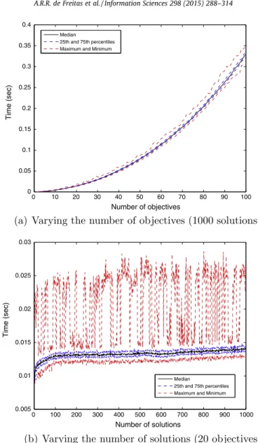
In order to show the relationship between the number of objectives and solutions,Fig. 8shows the relationship between the number of objectives and the number of solutions in a real execution of the algorithm. The quality of solutions were ran-domly generated numbers with uniform distribution between 0 and 1. For each parameter, we run 50 replicates in order to have the median values, the maximum and minimum values, and the 25th and 75th percentiles.

We can see that the execution time has a cubic relationship to the number of objectives and a linear relationship to the number of solutions. Those results are expected according to the time complexityOðnm3_{Þ. In the case ofFig. 8(b) we can also} see that even though the execution time varies linearly there is a significant constant amount of time that is spent regardless of the number of solutions.

7. Results of benchmark instances

7.1. Test instances

We have run experiments on the DTLZ benchmark instances[15]in order to show how the tree can represent the rela-tionship between objectives. For each instance, we use the algorithm PICEA-g[61]for 600 generations and 100 individuals to find a set of solutions for the problem with 20 objectives.

7.2. Results on the test function DTLZ-2

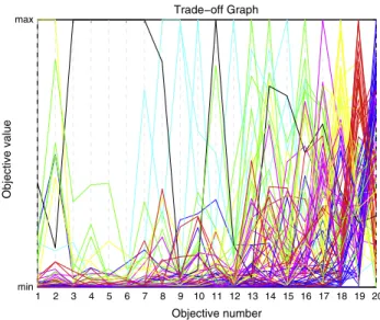
Fig. 9shows the parallel coordinate plot with the solutions in the objective space for the test function DTLZ2. In order to facilitate visualization, solutions are clustered with a PSA algorithm[50]into 7 clusters and solutions in the same clusters have the same colors.

Even when allied to the PSA clustering technique, the parallel coordinate approach does not facilitate the cognitive per-ception of the relationship between objectives.

InFig. 10, we plot the aggregation tree for the solutions to analyze the relationship between objectives. Objectivesf₁and f2are the two most harmonious ones, with 16.3% of non-parametric conflict, or 83.7% of harmony.

According to the tree and the harmony values, the next consecutive aggregations involve objectivesf3;f4in one branch, and thenf₁₀andf₉in another branch, respectively. Afterwards, there can be an aggregation of all those objectives into a new objective with only 5.6% of conflict.

As aggregations with lowest conflict happen first, we can find all the aggregations between the objectives until we have only one objective represented by the root node.

By looking at intermediate parent nodes, we can also monitor the relationship between groups of objectives. For instance, for the DTLZ2 instance, the groups which are most in conflict with one another are objectives (i)f16þf15, (ii)f17, (iii)f18, (iv) f19, (v)f20, and (vi) another group representing all other objectives. By looking at the branches that are close to the root node, the tree can help us make this kind of analysis for any number of clusters we want.

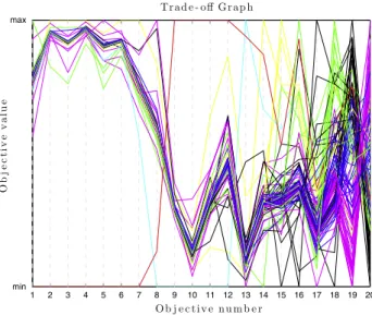
In the rearranged graph, it is easier to perceive the difference between groups recognized by the tree. Firstly, we have a group with objectives 10, 9, 2, 1, 3, 4, 7, 6, 8, 5, 11, and 12 in the middle of graph. According to the tree, those are the most harmonious objectives.

To the left and to the right of this middle group, there are two conflicting groups separated by the tree. Solutions with high values for the objectives on the left tend to have low values for objectives on the right and vice versa. Thus, the com-bination of the Aggregation Tree with the parallel coordinate plots can lead to a better global understanding of the relation-ships between absolute objective values.

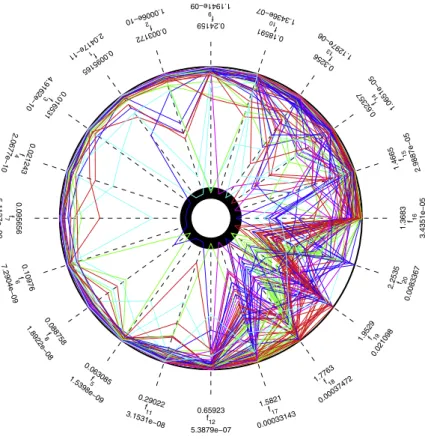
As mentioned in Section4, we can represent these results on a polar graph inFig. 12to analyze the absolute objective values. We can see in this graph that the groups clustered by the PSA algorithm roughly coincide with the groups identified by the tree. This is especially visible in objectives 17, 18, 19, 20.

7.3. Results on the test function DTLZ-5

Similarly to the DTLZ2 experiments,Fig. 13shows solutions for the DTLZ5 instance. In this instance, the relationship between adjacent objectives is already less chaotic than DTLZ2. This happens because the order of the objectives in this test problem is already in such a way that objective 2 is related to objective 1, objective 3 is related to objective 2, and so on.

0 10 20 30 40 50 60 70 80 90 100

0 0.05 0.1 0.15 0.2 0.25 0.3 0.35 0.4

Number of objectives

Time (sec)

Median

25th and 75th percentiles Maximum and Minimum

(a) Varying the number of objectives (1000 solutions)

0 100 200 300 400 500 600 700 800 900 1000

0.005 0.01 0.015 0.02 0.025 0.03

Number of solutions

Time (sec)

Median

25th and 75th percentiles Maximum and Minimum

(b) Varying the number of solutions (20 objectives)

This scenario is virtually never the case in a real-world problem, where the order of the objectives is usually arbitrary. To represent this scenario,Fig. 14shows the same solutions in a graph where the objectives have been randomly permutated. In this case, it is necessary to have a robust strategy to reorganize the objectives.

InFig. 15we have the aggregation tree for the DTLZ5 instance. In this tree, we have more well marked groups of conflict. The six biggest groups of conflict are (i) f18þf17, (ii) f16þf15þf14þf13þf5þf4þf9þf8þf7þf6þf12, (iii) f11þf10þf3þf2, (iv)f1, (v)f19, and (vi)f20.

The transposition of this data to the parallel coordinate plot representation and a polar graph is illustrated inFigs. 16 and 17. All the groups represented in the tree can be viewed in those representations. It is further noted that, in general, it is more difficult to optimize the objectives of the DTLZ5 instance.

1 2 3 4 5 6 7 8 9 10 11 12 13 14 15 16 17 18 19 20

min

Objective value

Objective number

Fig. 9.DTLZ2 – parallel coordinate plot.

As a result of space limitations, the results for all other DTLZ test problems are available fromwww.alandefreitas.com.

7.4. Decision-making scenarios

Here we present four examples of strategies in which the decision-maker can use the Aggregation Trees and their respec-tive polar graphs to restrict the preference area for the problem and search for an appropriate final solution.

16 15 14 13 10 9 2 1 3 4 7 6 8 5 11 12 17 18 19 20

min max

Fig. 11.DTLZ2 – rearranged parallel coordinate plot.

1.3683 f 16 3.4351e−05 1.4665 f15 2.9887e−05 0.623 57 _f14

1.0 651e− 05

0.32 56 f13 297e−06 1.1 0.18591 f 10 1.3436e−07 0.24159 f 9 1.1941e−09 0.003172 f 2 1.0006e−10 0.0 09 5165 f 1 2.0 41 7e −11 0.0 165 31 f 3 4.9 162 e− 10 0.021243 f 4 2.0677e−10 0.095656 f 7 5.1137e−09 0.10976 f 6 7.2904e−09 0.0 8875 8 f 8 1.89 22e −08 0.0 630 85 f 5 1.539 8e−0 9 0.29022 f 11 3.1531e−08 0.65923 f 12 5.3879e−07 1.5821_f 17 0.00033143 1.776 3 f18 0.0003 7472 1.9 529 f19 0.02 1098

2.2535f20 0.0083367

Of course, the examples provided here are only a small representative selection of strategies in which the decision-maker can use the information available to reach a definitive solution. There is a myriad of contextual ways in which this can be accomplished in a real-world problem. Also, the strategies presented here can be used and reused in any order as the prob-lem at hand demands.

7.4.1. Defining a harmony threshold for automatic objective aggregation

InFig. 12, we can see that there is a group of objectives (f10þf9þf2þf1þf3þf4þf7þf6þf8þf5þf11) which could be optimized in most solutions, with the exception of outliers. This group of objectives corresponds to the objectives which, on inspection of the tree inFig. 10, should be aggregated first.

As those are objectives that are in harmony, we aggregate all the original objectives that have less than 25% of conflict into a new objective functionf_a. We then optimize this new problem and the new results are presented inFigs. 18 and 19.

Apart from the aggregated objectives, we obtain a similar tree for all other objectives. In the polar coordinates plot, we can see thatfa, and its component objectives, can be optimized in most solutions.

7.4.2. Transforming some objectives into constraints

InFigs. 18 and 19, we can now see that the group formed by objectivesf12þfaþf13þf14þf15þf16represents the first recommendations for aggregation in the tree. Besides, all clusters identified by the PSA algorithm have solutions with sig-nificantly low values for all of those objectives.

Fig. 13.DTLZ5 – parallel coordinate plot.

10 4 18 6 7 5 8 15 1 17 20 3 9 14 13 2 19 16 11 12

min

max Trade−off Graph

Objective value

Objective number

Thus, we create a new constraint for the problem where only solutions withfi<0:28i2 fa;12;13;14;15;16gare consid-ered feasible. Assuming that, according to the decision maker, any value<0:2 is a reasonable value, we now remove those objectives and are left with a problem containing 4 objectives. The optimization of this new problem leads to the results in Figs. 20 and 21.

We now have a situation of extreme conflict between all the objectives. The most harmonious objectives aref17andf18, which still present 59.5% of conflict. For each cluster of solutions, there is at least one objective where this cluster presents poor quality.

7.4.3. Removing objectives

Given the high amount of conflict between all objectives in our problem with four objectives, let us consider that the deci-sion maker ceases to consider the objectivef20in order to explore the clusters of solutions that perform well on objectives f17;f18, andf19. By removing objectivef20and optimizing this new problem, we can then return a small set of solutions from which the decision maker can make a choice. This set of solutions is represented inFig. 22.

Fig. 15.DTLZ5 – Aggregation Tree.

We have now a small set of five optimized solutions that focus on a preference area defined by many strategies. This set can be readily analyzed by the decision-maker. For instance, the solution with best quality in f17 has objective values f17¼0:0000;f18¼0:0015, andf19¼0:0482. The quality of those solutions in the original objective functions is presented

1.298 f18

−0.58244

1.1299 f17

−0.28016 0.3 25 23 _f16

−0.1 9301

0.14

28 f15 −0.06

4.9 36 6e −0 7

f 4 −0 5

0.00107

96

f

9 −0.00

04 43 91

7.8592e−05

f

8

−0.00011772

3.1966e−05

f

7

−9.585e−05

4.5811e−06

f 6 −5.3685e−05

0.002 9857 f

12

−0_.002

47₄₄

0.002 40₉₁ f

11

−0.001

1189 0.002307 f

10

−0.00032105 1.9672e−07 f

3

−2.1528e−06

7.9427e−08f₂

−1.7269e−06

5.789

e−08

f1

−1.9

521e−07

2.1 178

f19

0.0 4018

3 2.2638f20

0.00874

Fig. 17.DTLZ5 – polar graph.

inFig. 23. There is a great amount of diversity between those solutions, but it is important to remember that many of the aggregated objectives are only represented over a narrow range of values now as they have become constraints.

7.4.4. Optimizing large groups of relevant objectives

In this subsection, we reveal another possibility for the use of the information available inFigs. 20 and 21. This time, instead of removing the objectivef20, which is presented by the tree as the objective with the most conflict with other objec-tives, we optimize two groups of final objectivesfb¼f17þf18þf19 andf20 in order to explore and visualize the conflict between them.

Fig. 24illustrates the quality of the solutions in 2 dimensions. As representative examples, the solutions with the best value in each the objectives have objective valuesfb¼0:0085;f20¼1:8822, andfb¼0:6363;f20¼0:0148. If the decision-maker chooses a solution with median values for both objectives, this solution has objective valuesfb¼0:3132;f20¼1:4001. Also, the decision-maker can visualize the quality of those solutions in the original objectives, as it is shown inFig. 25. Again, it might be difficult to analyze all solutions with the original objectives as many different strategies have been employed to reduce the preference area in the objective space. However, we can still recognize the objectives which were

1.4864 f

18

0.0029376

1.6956 f17

4.3117e−05 0.73153

f

12 2.6532e−06

0.12088 f a

2.1713e−08

0.77797 f 13

2.5019e−07

1.2479

f

14

3.9569e−05

1.7384 f 15 1.6314e−07

1.2301 f 16 0.0001086

2.206 f₁₉

0.00020208

2.1879f20

0.025322

Fig. 19.DTLZ2 (10 objectives) – polar graph.

restricted to a short range of values as constraints. Still, we can see the clear conflict between objectivef20and all other adjacent objectives in this set of solutions.

8. Discussion and future work

This paper proposes a tree-based method to visualize the relationship between objectives in many-objective problems. The trees are based on measures of conflict and harmony between objectives to infer their reducibility. In addition, a mea-sure of region of conflict is used to color the aggregation nodes to represent where non-parametric conflict is occurring most.

1.8481 f

18

0.00071424

1.8858

f

19

0.00067582

2.03

f₂₀

0.0060111

Fig. 21.DTLZ2 (4 objectives) – polar graph.

0.31779

f19

0.002737

0.02064 f 17

6.6832e−06

0.0074431

f 18 0.0010744

The first main advantage of the method is the facility of iterative reduction to show the relationship between groups of objectives, regions of conflict, and their reducibility. The measure of conflict also informs the decision maker of the size of the penalty involved in the reduction of those objectives.

A second important feature is that all metrics used are non-parametric and can be generally used for any many-objective problem, being independent of any kind of specific linear or non-linear relationship between the objectives. The

represen-0.02064 f17 6.6832e−06 0.03194 f15 0.0001493 0.001 3389 f13 31 _1.6

e−05

0.0 00 56

637 f10 16 3.6

1e− 07 0.00014041 f 9 3.1829e−06 0.00051225 f 8 1.5843e−06 0.00010689 f 7 3.5395e−08 9.9 34 9e −06 f 2 5.1 858 e− 09 2.17 21 e−05 f 3 4.2 36 9e−0 8 8.8786e−06 f 1 2.7352e−09 2.2324 f 20 1.7435 0.023567 f 16 0.00056391 0.01 64 6 f 14 2.0827e−0 6 0.0010 914 f 12 5.1₂₄ e− 06 0.00081109 f 11 7.9308e−06 0.00012816 f 6 2.5035e−09

8.8496e−05f₅

1.3907e−08 2.1948e− 05 f4 6.988 2e−0 9 0.0 074 431 f18 0.00 1074 4 0.31779f19

0.002737

Fig. 23.DTLZ2 (5 solutions – 20 objectives) – polar graph.

0 0.1 0.2 0.3 0.4 0.5 0.6 0.7

0 0.2 0.4 0.6 0.8 1 1.2 1.4 1.6 1.8 2 f

17+f18+f19

f 20

tation of iterative aggregation also makes it convenient for the decision maker to choose which objectives can be effectively grouped. The measures of conflict make this decision easier.

The tree can also be used with (i) only non-dominated solutions to infer and analyze the relationship between the objec-tives on the Pareto front and therefore represent which objecobjec-tives have the possibility of being optimized in a group, (ii) any set of random solutions to analyze the presence or absence of inherent harmony between objectives for any solutions and indicate which objectives could be reduced, or (iii) even solutions limited to a preference area in order to have a more spe-cific analysis of the objectives in that area. Either way, unless we already have a very restricted preference area, as the num-ber of objectives grows, this difference has a tendency to disappear because most solutions tend to be non-dominated.

Given the possibility of analysis of a Pareto front and a comparison between many objectives being plotted, the proposed approach is very simple to implement and has a low computational cost. In the case of a MOEA that uses objective reduction, a partially constructed tree could be used to indicate objectives to be reduced with low computational cost.

The iterative step of the algorithm always chooses the two most harmonious objectives in a greedy fashion. This choice may not always lead to the best tree if we consider the objectives that have already been paired. For this reason, the order of reduc-tion to this objective reducreduc-tion problem might be only a local optimum in relareduc-tion to the number of objectives to be reduced. An alternative approach might be to sum the conflict of all the children of a compound objective when choosing the next aggregation, in order that all aggregations are considered on a given iterative step.

As the algorithm uses iterative steps of objective aggregation, it is also possible that other techniques of objective reduction can be tested as the main aggregation method for the tree.

It is likely that the order of aggregation of the objectives and new measures of harmony that consider more than two objectives per aggregation will lead to a combinatorial model to be optimized. In many-objective optimization, from the point of view of Pareto-dominance, most points are on the Pareto front anyway. Thus, we might consider that estimating a good tree to the decision maker in order that they can narrow their preference area may be more important than being concerned with applying optimization algorithms to the problem itself unless there is a good measure of comparability between the objectives. Optimization could be better utilized, applied to the trees instead. Thus, estimating an optimal tree representing an optimal reduction strategy could become a primary goal of these many-objective problems.

Acknowledgements

This work has been supported by the Brazilian Agencies State of Minas Gerais Research Foundation – FAPEMIG, Coordi-nation for the Improvement of Higher Level Personnel – CAPES, National Council of Scientific and Technological

Develop-1.5431 f 18 0.00080462 0.44261 f17 0.00049652 0.0108 65 f11 7.7865e−08 0.00318

89 f9 058e−0 6.7

406 15 f 7 0.0 01 000 6 f 6 1.3 08 5e −07 0.00018848 f 5 1.4854e−08 0.00013655 f 2 6.5698e−10 0.00025704 f 1 1.2011e−09 0.00 01968 2 f 3 6.6 365e−09 0.00021 57₃ f 4 1.3 04e− 08 0.10847 f 14 0.00011796 0.07615 f 13 1.1311e−05 0.13123_f 15 7.6808e−05 0.158 7 f16 0.000 10204 1.7 156 f19 0.0 0234 67 1.8822f20

0.014798