Characterization of an OPCPA laser amplifier based on the nonlinear crystal YCOB

Joana Andreia Casanova Ferreira Alves

Licenciada em Ciências de Engenharia Física

Characterization of an OPCPA laser amplifier

based on the nonlinear crystal YCOB

Dissertação para obtenção do Grau de Mestre em Engenharia Física

Orientadores: Ana Gomes Silva, Professora Auxiliar, FCT-UNL Gonçalo Figueira, Professor Auxiliar, IST-UL

Júri:

Presidente: Isabel Catarino,

Professora Auxiliar, FCT-UNL

Arguentes: Dawei Liang,

Professor Auxiliar, FCT-UNL

Vogais: Gonçalo Figueira, Professor Auxiliar,

Characterization of an OPCPA laser amplifier based on the nonlinear crystal YCOB

Copyright © Joana Andreia Casanova Ferreira Alves, Faculdade de Ciências e Tec-nologia, Universidade Nova de Lisboa.

Agradecimentos

Antes de mais gostaria de agradecer aos meus orientadores por me terem dado a oportunidade única de trabalhar numa área tão interessante e desafiante como a óptica e os fenómenos associados à produção de sistemas laser intensos; à Professora Ana Gomes Silva por ter estabelecido esta colaboração e ao Professor Gonçalo Figueira por me ter acolhido de forma tão agradável e simpática no seu grupo. Agradeço a ambos, de igual modo, o apoio imprescindível ao longo de todo o trabalho incluindo a fase de pre-paração de dissertação, a orientação sabedora bem como as sugestões para o desen-volvimento deste trabalho, no esclarecimento de dúvidas e discussões científicas. Não menos importante foi a sua total disponibilidade e incentivo permanente à descoberta das minhas perspectivas futuras. A amizade demonstrada e o conhecimento transmitido foram de uma grande inspiração e motivação para mim.

No entanto, não poderia também deixar de agradecer ao Celso João por ter acom-panhado todo o meu trabalho experimental e teórico assim como pelas longas discussões e esclarecimentos que paciente e alegremente prestou até ao surgimento das soluções. Ao Hugo Pires por ter contribuído para a minha melhor compreensão sobre os conceitos não lineares do amplificador paramétrico, bem como pelas histórias bem contadas que divertiam o grupo durante as longas horas de trabalho no laboratório.

Agradeço ao IPFN por me ter disponibilizado os meios necessários à realização do trabalho nas melhores condições e a todos os elementos do GoLP em especial alunos, técnicos, professores e funcionários por me terem recebido calorosamente.

Abstract

The work described in this thesis was performed at the Laboratory for Intense La-sers (L2I) of Instituto Superior Técnico, University of Lisbon (IST-UL). Its main contribu-tion consists in the feasibility study of the broadband dispersive stages for an optical parametric chirped pulse amplifier based on the nonlinear crystal yttrium calcium oxi-borate (YCOB). In particular, the main goal of this work consisted in the characteriza-tion and implementacharacteriza-tion of the several optical devices involved in pulse expansion and compression of the amplified pulses to durations of the order of a few optical cycles (20 fs). This type of laser systems find application in fields such as medicine, telecommuni-cations and machining, which require high energy, ultrashort (sub-100 fs) pulses.

The main challenges consisted in the preliminary study of the performance of the broadband amplifier, which is essential for successfully handling pulses with band-widths exceeding 100 nm when amplified from the µJ to 20 mJ per pulse. In general, the control, manipulation and characterization of optical phenomena on the scale of a few tens of fs and powers that can reach the PW level are extremely difficult and challenging due to the complexity of the phenomena of radiation-matter interaction and their non-linearities, observed at this time scale and power level.

For this purpose the main dispersive components were characterized in detail, specifically addressing the demonstration of pulse expansion and compression. The tested bandwidths are narrower than the final ones, in order to confirm the parameters of these elements and predict the performance for the broadband pulses. The work per-formed led to additional tasks such as a detailed characterization of laser oscillator seed-ing the laser chain and the detection and cancellseed-ing of additional sources of dispersion.

Resumo

O trabalho descrito nesta dissertação foi realizado no Laboratório de Lasers Intensos (L2I) do Instituto Superior Técnico da Universidade de Lisboa (IST/UL), tendo contribuído para o desenvolvimento de um amplificador laser, do tipo amplificação óptica paramétrica de impulsos dispersos baseado num cristal não-linear de oxi-borato de ítrio-cálcio (YCOB). Em particular, o principal objectivo deste trabalho consistiu na caraterização e implementação do sistema no que se refere à capacidade de expandir e comprimir impulsos laser para durações da ordem dos poucos ciclos ópticos (20 fs). Este tipo de sistemas laser encontra aplicação em campos como medicina, telecomunicações e maquinação, que requerem impulsos ultra-curtos (sub 100 fs) de alta energia.

O desafio residiu no estudo prévio, mas essencial para uma manipulação bem sucedida, de impulsos com largura de banda superior a 100 nm (com comprimento de onda central a 800 nm) quando amplificados de 4 ordens de grandeza (dos µJ a 20 mJ). Na realidade, o controlo, a manipulação e a caraterização dos fenómenos ópticos à escala de poucas dezenas de fs e com potências na ordem dos PW são extremamente complexos, devido aos complexos fenómenos que ocorrem como consequência da inte-racção radiação–matéria e a não-linearidade dos mesmos.

Com esse propósito foram caracterizados, de forma detalhada e rigorosa, os prin-cipais componentes dispersivos, incluindo a verificação da compressibilidade para lar-guras de banda menores que as finais de forma a garantir o bom desempenho destes elementos e prever a resposta para os impulsos pretendidos. A execução do trabalho obrigou a abordagens complementares como a caracterização do oscilador que alimenta a cadeia laser e à detecção e supressão de outras causas de dispersão.

Contents

AGRADECIMENTOS... VII

_!

ABSTRACT ... IX

_!

RESUMO ... XI

_!

CONTENTS ... XIII

_!

LIST3OF3FIGURES ...XV

_!

LIST3OF3TABLES ... XIX

_!

LIST3OF3ABBREVIATIONS ... XXI

_!

LIST3OF3SYMBOLS... XXIII

_!

INTRODUCTION ... 1

_!

1.1!CHIRPED!PULSE!AMPLIFICATION...2

!

1.2!OPTICAL!PARAMETRIC!CHIRPED!PULSE!AMPLIFICATION...2

!

1.3!MOTIVATION!OF!THE!THESIS...4

!

1.4!THESIS!WORK!OUTLINE...4

!

PULSE3STRETCHING3AND3COMPRESSION ... 7

_!

2.1!DISPERSION...7

!

2.2!PULSE!DURATION!AFTER!DISPERSION...9

!

2.3!GROUP!DELAY!DISPERSION!AND!THIRD!ORDER!DISPERSION...11

!

2.3.1%Transparent%media ...13

!

2.3.2%Transmission%grating%pair ...15

!

2.3.3%Brewster%prism%pair...18

!

2.3.4%Chirped%mirror%pair ...20

!

2.4!STRETCHER>COMPRESSOR!ASSEMBLY...21

!

3.1!AUTOCORRELATION... 23

!

3.1.1%Background>free%intensity%scanning%autocorrelator ...25

!

3.2!FREQUENCY>RESOLVED!OPTICAL!GATING... 27

!

3.2.1%Second>harmonic%generation%FROG ...28

!

STRETCHING3AND3COMPRESSION3DEVICES ... 31

_!

4.1!NUMERICAL!SIMULATIONS... 31

!

4.1.1%SF11%glass%block...32

!

4.1.2%Transmission%grating%pair ...34

!

4.1.3%SF11%Brewster%prism%pair ...36

!

4.2!EXPERIMENTAL!CHARACTERIZATION... 38

!

4.2.1%Oscillator...39

!

4.2.2%Oscillator%and%FI ...43

!

4.2.3%Oscillator,%FI,%double%pass%in%SF11%rod%and%transmission%gratings ...44

!

4.2.3%Oscillator%and%prisms ...48

!

4.2.4%Oscillator,%FI%and%prisms ...50

!

EXTRAPOLATION3FOR3THE3OPCPA3SYSTEM ... 53

_!

5.1!OPTICAL!PARAMETRIC!CHIRPED!PULSE!AMPLIFICATION... 53

!

5.2!SEED!AND!PUMP!PULSES... 54

!

5.3!STRETCHER>COMPRESSOR!ASSEMBLY... 55

!

CONCLUSIONS3AND3FUTURE3WORK ... 57

_!

6.1!FUTURE!WORK... 58

!

REFERENCES... 59

_!

List of figures

!

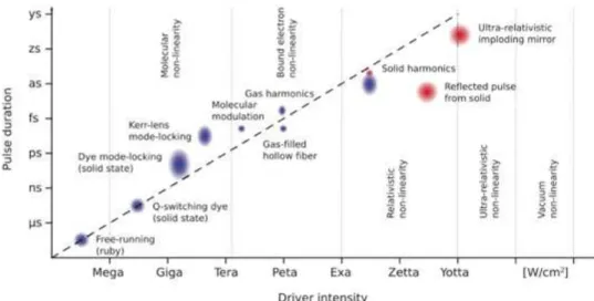
Figure 1.1: Progress in laser pulse intensity and duration. ...1

!

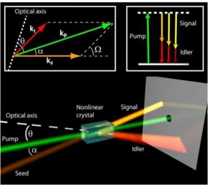
Figure 1.2: Schematic representation of the OPA main principle. The geometry represents a noncollinear interaction, where there is a small angle between the pump and signal beam directions...3

!

Figure 2.1: Examples for the introduction of quadratic and cubic phases on the pulse. Upper box: FTL pulse which corresponds to a zero spectral phase; middle box: insertion of a positive quadratic phase, broadening the pulse in time; lower box: insertion of a negative cubic phase leading to a stronger pulse preceded by an increasing pulse sequence...11

!

Figure 2.2: Schematic representation of the formalism used to calculate the spectral phase. The geometry represents two different wave vectors k_{1 and} k_{2, their projection over an arbitrary vector} R_{, and the optical}

path difference between them (this is, the phase lag δ). ...12

!

Figure 2.3: Schematic diagram of a transmission grating pair. Angular dispersion causes the redder components of the pulse to travel a longer distance than the bluer components, resulting in a negative chirp. ...16

!

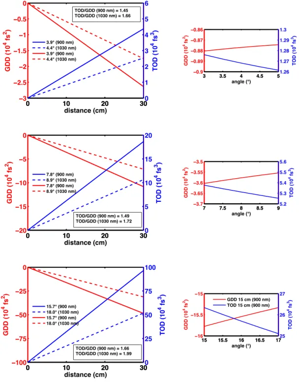
Figure 2.4: Variation of GDD (blue lines) and TOD (red lines) generated by 150 g/mm (top), 300 g/mm (middle) and 600 g/mm (bottom) grating pair compressors at 900 nm (solid line) and 1030 nm (dashed line) for fixed Littrow angles at different perpendicular distances between gratings (left) and for a fixed distance of 15 cm at different near Littrow incident angles (right). TOD/GDD ratio for is added to the different gratings. ...17

!

Figure 2.5: Schematic diagram of a prism pair. In this case, angular dispersion and material dispersion inside the second prism can be tuned to provide desired amounts of GDD and TOD. ...19

!

Figure 2.6: Variation of GDD (blue lines) and TOD (red lines) generated by BK7 (top) and a SF11 (bottom) prism pair compressors at 900 nm (solid line) and 1030 nm (dashed line) for fixed apex angles (59° for the first compressor and 67° for the latter) at different apex-to-apex distances between prisms (left) and for a fixed distance of 15 cm with different material insertion length (right). TOD/GDD ratio is added to the different gratings...20

!

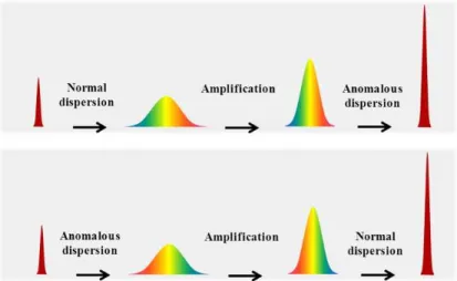
Figure 2.7: Schematic representation of the operation principle of a chirped mirror. Longer wavelengths will experience longer optical paths since they penetrate deeper into the mirror structure thus resulting in anomalous dispersion of the pulse...21

!

Figure 2.8: Schematic representation of the two principles of stretching and compressing the pulse. Upper box: insertion of positive GDD and down-chirp compensation (configuration used in this work); lower box: initial negative GDD is cancelled by an up-chirp compressor...22

!

Figure 3.1: Schematic representation of an intensity second-harmonic autocorrelator using a Michelson interferometer and a SHG crystal. The pulse is split in two on a Michelson interferometer and is recombined in a second order nonlinear crystal generating a new signal. ...24

!

Figure 3.2: Examples of intensity and interferometric autocorrelations of a Gaussian pulse. Left box: graphic of a FTL Gaussian input pulse; right box: normalized fringe-resolved interferometric autocorrelation and intensity autocorrelation. ...24

!

arm is continuously changed. This allows the construction of the autocorrelation function after recombining the pulses in a second order nonlinear crystal. ... 26

!

Figure 3.4: Schematic representation of the optical path of the pulses on the scanning intensity autocorrelator setup used to characterize the pulses from the oscillator. The input pulse (red) is split in two: one part goes through a fixed path length (orange) and the other suffers a periodically delay caused by a mechanical shaker (salmon); after crossing both parts inside a nonlinear crystal the SHG is generated (green) and is sent to the photomultiplier. ... 26

!

Figure 3.5: Example of a visualised autocorrelation on the oscilloscope display. The superposition of the two pulses in the nonlinear optical medium produce a slow (ms-scale) detection signal that corresponds to a coherent addition of both the electric fields... 27

!

Figure 3.6: Schematic representation of the frequency-resolved optical gating main principle. The test pulse

E(t) and the gate pulse G(t-τ) interact inside a nonlinear medium (left) slicing the test pulse (right). ... 28

!

Figure 3.7: Schematic representation of a second-harmonic generation frequency-resolved optical gating using a Michelson interferometer and a SHG crystal. The SHG-FROG consists in a standard SHG-based noncollinear intensity autocorrelator with photodetector replaced by a spectrometer. ... 28

!

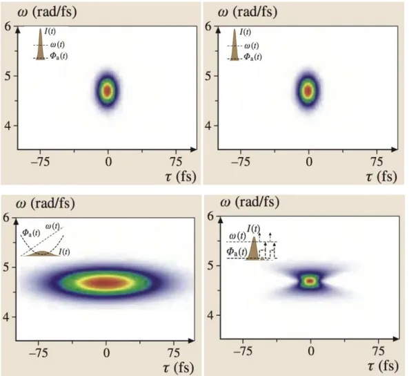
Figure 3.8: Examples of frequency-resolved optical gating trace for common ultrashort pulse distortions (shown on the top left of each box). Upper left box: FROG trace of a FTL 10 fs pulse; upper right box: FROG trace remains the same as only first order dispersion value was introduced; lower left box: second order dispersion term creates a FROG trace stretched in time (note that it is not possible to tell whether it is normal or anomalous dispersion); lower right box: FROG trace of a pulse with third order dispersion term gives us an unintuitive spectrogram since we have a symmetrical image... 29

!

Figure 3.9: Examples of FROG traces of a pulse with GD, GDD and TOD using two different FROG techniques. Left box: FROG trace using polarization gate FROG; right box: using SHG FROG it is not possible to distinguish between positive or negative GDD nor between pre- or post-pulses. ... 30

!

Figure 4.1: Output pulse duration versus initial pulse duration for different values of GDD. As the input pulse width becomes shorter, the effects of GDD become more pronounced, since the pulse broadening and chirping is stronger for pulses with broader bandwidths. (Note that the values in this graphic correspond to the FWHM pulse duration defined in our work as Δt). ... 32

!

Figure 4.2: Schematic of the several orders of diffraction for a 300 g/mm transmission grating with an incident angle γ = 32º at λ = 1030 nm. θ1 = 57.03º θ0 = 32º θ-1 = 12.76º θ-2 = -5.05º θ-3 = -23.4º θ-4 = -44.92º; with θ-1 being the most efficient diffraction order. ... 35

!

Figure 4.3: Layout of the 300 g/mm grating pair compressor with γ = 32º at λ = 1030 nm. ... 36

!

Figure 4.4: Prism compressor compact geometry... 38

!

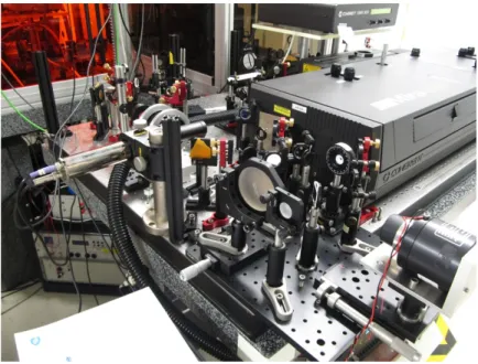
Figure 4.5: Oscillator Coherent Mira 900 F. Top box: Ti:sapphire laser cavity pumped by a Verdi-V 10; middle box: schematic representation of the oscillator cavity (M – mirror; P – prism; L – lens; BRF – birefringent filter; OC – output coupler); left bottom box: Ti:sapphire crystal mount; left bottom box: prism compressor... 40

!

Figure 4.6: Optical path in the prism compressor inside the oscillator. Translating the second prism in the same direction of its main axis will insert or remove material dispersion that can change the output of the prism compressor. ... 41

!

Figure 4.7: Calculated (red) and measured (blue) values of the output pulsewidth for the different measured prism insertion quantities. Linear fit of the calculated (dashed red line) and measured (dashed red blue) is also shown. ... 42

!

Figure 4.8: Variation of the GDD (red) and output durations (blue) with prism insertion. Top box: Variation of the GDD and output durations with prism insertion in the region of the experimental data; bottom box: variation of the GDD and output durations with prism insertion in large range. The measured points (black circles) and the experimental linear fit (dashed black line) can be compared with the experimental output duration vs. prism insertion curve. ... 43

!

Figure 4.9: Experimental setup of the stretcher-compressor assembly to study grating pair. The pulse that leaves the oscillator pass trough FI, after in the grating compressor, then twice in the SF11 rod and finally they will be sent to the autocorrelator. The same setup is shown in different positions. ... 46

!

Figure 4.11: Experimental output pulse durations vs. distances between gratings (blue points) and the corresponding fit (red line). This mathematical fit considers also the TOD since the input pulse is only a few tenths of fs long and has a large TOD value. ...48

!

Figure 4.12: Experimental setup of the stretcher-compressor assembly to study prism pair. In order to understand the problems in the compression of the pulses using prism pair we chose to verify its capability in compressing a small value of positive dispersion introduced by the insertion of its own material thus the pulse that leaves the oscillator directly goes to prism compressor and then to the autocorrelator. The same setup is shown in different positions. ...49

!

Figure 4.13: Experimental output pulse durations for different values of prism insertion (blue points) and the corresponding fit (red line)...50

!

Figure 4.14: Experimental output pulse durations for different values of prism insertion (blue points) and the corresponding fit (red line) to compensate the pulses coming from the oscillator after passing the FI. ...51

!

Figure 5.1: Global layout of ultrabroadband OPCPA system. Top box: CPA pump laser based on a

double-stage, diode pumped CPA system; middle box: generation of signal pulse based on white light continuum generation (WLG) in bulk media; bottom box: double stage OPCPA system based on YCOB. ...54

!

List of tables

Table 2.1: Calculated dispersion coefficients for SF11 glass and respective TOD/GDD ratios. ...14

!

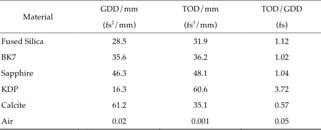
Table 2.2: Dispersion coefficients for different materials at 900 nm wavelength and respective TOD/GDD ratios...14

!

Table 2.3: Sign of dispersion contributions of the most common optical components of a stretcher-compressor assembly...22

!

Table 4.1: Calculated dispersion coefficients and correspondent output pulse duration for an FWHM FTL =

60 fs introduced by the FI, by 1 to 4 passes through the 12.5 cm SF11 glass and by the FI together with the single and multiple pass through the SF11 glass block...33

!

Table 4.2: Calculated autocorrelation and output pulse duration (assuming a Gaussian profile) for the oscillator input pulses for different GDD and TOD values...34

!

Table 4.3: Calculated dispersion coefficients introduced by the grating pair compressor with an incident angle of 31.7˚ vs. perpendicular gratings separation Lg. ...35

!

Table 4.4: Calculated dispersion coefficients introduced by the SF11 prism pair compressor with an apex angle of 59˚, 1000 nm wavelength at apex vs. apex-to-apex distance Lp....37

!

Table 4.5: Calculated dispersion coefficients introduced by the SF11 prism pair compressor with an apex angle of 59˚ vs. apex-to-apex distance Lp and SF11 crossed length lm. ...37

!

Table 4.6: Theoretical values for different optical elements in order to determine the total constant value of GDD inside the oscillator...42

!

Table 4.7: Theoretical values for different optical elements in order to determine the total constant value of TOD inside the oscillator. ...47

!

Table 5.1: GDD and TOD calculated for pulse stretching and compression of the pulse. ...56

!

Table 6.1: Comparison between the GDD and TOD introduced per mm by the current optical elements for

List of abbreviations

BBO Beta barium borate (β-BaB2O4)

CEP Carrier envelope phase CPA Chirped pulse amplification CVBG Chirped volume Bragg grating

DKDP Potassium dideuterium phosphate (KD2PO4)

DOM Disperse-O-Matic

FI Faraday isolator

FPM femtoPulse Master

FROG Frequency-resolved optical gating FTL Fourier-transform limit

FWHM Full-width at half the maximum intensity

GD Group delay

GDD Group delay dispersion L2I Laboratory for Intense Lasers OPA Optical parametric amplification

OPCPA Optical parametric chirped pulse amplification SHG Second-harmonic generation

SHG-FROG Second-harmonic generation frequency-resolved optical gating TBWP Time-bandwidth product

TGG Terbium gallium garnet (Tb3Ga5O12)

TOD Third order dispersion

YCOB Yttrium calcium oxyborate (YCa4O(BO3)3)

List of symbols

A Amplitude

Bn Sellmeier coefficients

Cn Sellmeier coefficients

c Speed of light in vacuum

E Electric field

G Electric field of the gate pulse

g Diffraction grating groove spacing

I Intensity

k _{Wave vector}

l Optical path length

la Optical path length between two prisms

lm Optical path length inside optical material

n Refractive index

n0 Refractive index at the central frequency or wavelength

Pavg Average power

R _{Arbitrary vector}

t Time

γ Incident angle

Δt Full temporal width at half the maximum intensity

ΔtAC Full autocorrelation temporal width at half the maximum intensity Δλ Spectral bandwidth (nm)

δ Phase lag

θ Angle of diffraction/refraction

λ Wavelength

λ0 Central wavelength

ν Frequency (Hz)

τ Half temporal width at 1/e2 _{of the maximum intensity}

φ Phase

φa Angular dispersion/phase

φm Material dispersion/phase

φn Phase terms of the phase Taylor expansion

ω Angular frequency (rad)

Introduction

More than 50 years of laser technology improvement – including the definition and implementation of important concepts as Q-switching in 19611_{, mode-locking in 1965}1

and chirped pulse amplification (CPA) in 19852 _{–, proved to be a milestone in science,}

enabling new areas of fundamental and applied physics and also finding new applica-tions in chemistry, biology, medicine, telecommunicaapplica-tions, industry, meteorology, se-curity and many others. During this evolution, not only the increasing of laser pulse en-ergy was boosted but also the decreasing of its duration assumed extreme values, lead-ing to even higher and higher output peak power laser systems and to a new area of re-search: ultrafast science. In this new field ultrashort pulses of the order of few cycles are used to generate coherent harmonic radiation and attosecond pulses that can be used for example in visualization of biology and chemistry samples at atomic scales, and high-field physics.3

Figure 1.1: Progress in laser pulse intensity and duration.4

1.1 Chirped pulse amplification

Ultrashort pulses have a typical temporal width between 10-12 _{to 10}-14 _seconds

al-lowing the generation of high peak optical powers even with relatively low pulse ener-gies.5 _{The generation of ultrashort pulses was possible with the improvement of}

mode-locking techniques and the lensing effect. This led to the development of the Kerr-lens mode-locked Ti:sapphire laser,6 _{a laser with a Ti:sapphire gain medium pumped by}

a solid state diode laser and a cavity that is preferentially made to lase in a pulsed mode rather than in a continuous wave mode. Due to a focusing process, fast self-amplitude modulation is achieved, generating mode-locked pulses and after dispersion compensation inside the cavity by a prism pair compressor, ultrashort pulses are re-leased. As ultrashort pulses started to be commonly available there was an interest in finding new amplification techniques since laser amplifiers were restricted at that time to directly amplifying only longer input pulses. In 1985 one of the most important concepts for producing high-intensity, ultra-short laser pulses was introduced by Strickland and Mourou, based on pulse stretching and compression, overcoming the problem of nonlin-ear effects and optical damage – the chirped pulse amplification (CPA) technique. This concept consists in three steps: (1) stretching the pulse in time by passing it through a dispersive delay line, proportionally decreasing its peak intensity; (2) amplifying this chirped pulse in a conventional way; (3) compressing the pulse to its transform-limited duration increasing proportionally its peak intensity using another dispersive delay line that will compensate the induced chirp.2 _{Stretching and compression can be achieved by}

optical elements such as bulk material, gratings, prisms, grisms and chirped-mirrors, enabling a dramatic increase in the maximum achievable peak intensity.7

1.2 Optical parametric chirped pulse amplification

Pulse stretching and compression are one of the most crucial stages in chirped pulse amplifiers, especially for few-cycle pulse amplifiers.8 _{Although CPA systems have}

enabled the development of high-energy few-cycle pulses they can have several issues such as narrow spectral bandwidth, gain narrowing and amplified spontaneous emis-sion, currently limiting them to the generation of PW-level pulses.9 _{About 20 years ago}

an alternative technique for the generation of high-energy ultrashort pulses also based in the concept of stretching and compressing the optical pulses was introduced – optical parametric chirped pulse amplification (OPCPA).7,10,11,12,13 _{Although recently introduced,}

OPCPA has already shown the potential to improve the laser pulse energy and duration, as well as repetition rate and pulse contrast, to values not previously achieved with con-ventional amplification.13

OPCPA results from a combination of CPA and another laser amplifier technology named optical parametric amplification (OPA).14 _{The conjugation of CPA with a}

trans-fers energy to a weaker, lower frequency input wave (seed/signal pulse) generating also an auxiliary wave (idler pulse) due to energy and momentum conservation – that is OPA, is currently providing solutions to several of the CPA limitations, envisaging an output power up to the multipetawatt level.14 _{Figure 1.1 represents the principle of three}

wave-mixing phenomena, described in terms of wave vectors and an energy diagram, showing the energy conservation during the process and the phase matching condition.

OPCPA has a number of advantages such as high gains per single pass, broad gain bandwidths, high quantum efficiency, low thermal deposition, reduced amplified spon-taneous emission and high amplified signal beam quality with high contrast ratio.11 _All

these highly desirable properties have led to a wide dissemination of OPCPA-based sys-tems at high power laser laboratories around the world.

Figure 1.2: Schematic representation of the OPA main principle. The geometry represents a noncollinear interaction, where there is a small angle between the pump and signal beam directions.5

Two of the most important design choices for an OPCPA system are the pump technology and an appropriate nonlinear crystal, as they will determine the output char-acteristics of the system, such as average power, pulse energy and amplification band-width.13_{A common option is to use a CPA laser as a pump, and actually the highest}

pulse energies are generated by the use of flashlamp-pumped amplifiers,15 _{while the}

highest average powers are allowed by the use of fiber-based pump technology.16

technology that allows both high pulse energy and high repetition rates, thereby enab-ling high average power as well.

For the OPA part, there are also a number of possible crystal choices, with beta-barium borate (BBO)18 _{and lithium triborate (LBO) being two of the most used}

non-linear crystals, thanks to their high non-non-linear coefficients and broad gain bandwidths. However, such choices are limited by the currently available crystal apertures, restricting their use to the pre-amplifier stages of high-energy laser systems. On the other hand, there are several examples that use large aperture potassium dideuterium phosphate (DKDP) crystals;19 _{however its low non-linear coefficient and poor thermo-optic}

proper-ties make it inadequate for high average power operation.Theborate crystal yttrium cal-cium oxyborate (YCOB)20 _{is a relatively recent and interesting alternative with a high}

nonlinear coefficient, large growth size capability and high damage threshold.21

1.3 Motivation of the thesis

A tabletop OPCPA system is being developed at the Laboratory for Intense Lasers (L2I)21 _{to complement the laser amplifier technology currently available – a hybrid,}

flash-pumped Ti:sapphire/Nd:glass-based CPA.22 _{The compactness and efficiency of this new}

system, together with a higher repetition rate, shorter pulses and lower pulse energies but comparable peak intensities, will allow for new experimental research of physical processes at the femtosecond scale in a much faster regime.

With the basic layout, delay lines and amplification stages of this OPCPA system already implemented, the compression and characterization of the output pulses are now some of the main concerns of the project. A stretching and compression setup had been proposed consisting in a SF11 glass block stretcher and a combination of prism pair and grating pair compressors, requiring a careful study and choice of the optimum pa-rameters for the optical devices to efficiently stretch and compress the signal pulses be-fore and after the two YCOB crystals bebe-fore applying them on the OPCPA.

In fact, the last part of the OPCPA system and the main concern of this project is the stretching and compression of the amplified pulses, since for a final pulse with a duration of just a few tens of femtoseconds higher dispersion orders have to be compen-sated for compression close to the Fourier transform limit (FTL). Because we are dealing with very broadband spectra, even a small amount of these dispersion orders will cause a relevant increase in the pulse duration.

1.4 Thesis work outline

around the following three major goals, which will be presented and discussed along the next chapters:

(1) to perform numerical simulations for different parameters of the gratings and prisms configuration;

(2) to characterize experimentally the dispersion caused by the most relevant opti-cal components to be used in the setup with the available bandwidth (~20 nm) coming directly from the oscillator;

(3) to compare the experimental results with the predicted ones and extrapolate them to wavelength intended for OPCPA operation (650-1000 nm). With this data we can evaluate whether the design and dispersive optical media used are appropriate for the compression of the OPCPA output pulses down to 20 fs du-ration.

After this short introduction (Chap. 1), the thesis continues with the theory under-lying pulse stretching and compression (Chap. 2), which includes the concepts of mate-rial and angular dispersion, Taylor expansion of the spectral phase up to several orders, as well as their influence on the temporal profile of the pulse. The optical materials that are proposed to generate and compensate the dispersion of the optical pulses are also introduced in Chapter 2.

Chapter 3 is devoted to the characterization of ultrashort pulses, that is to the the-ory of ultrashort pulse measurement and a description of the measuring diagnostics used in the experimental work. The characterization of the pulses to be stretched and compressed is presented at the end of this chapter.

In Chapter 4 the theoretical study and experimental characterization of the stretch-ing and compression optical media are reported. The experimental data is followed by an analysis and discussion.

Chapter 5, although short, addresses the important issue of the extrapolation to the operating bandwidth of the OPCPA system. Based on the previous results we analyse and discuss the expected performance and suitability at the effective projected parame-ters.

Pulse Stretching and Compression

Pulse stretching and compression are only made possible by the introduction of dispersive optical setups of opposite signs. Since ultrashort pulses, characterized by their short durations, have large frequency bandwidths the concept is based on generating a controllable delay for each frequency and so expanding the pulse in time; also, removing the same delay we can then have a pulse that is compressed in time. The insertion of this delay can be achieved by propagating the optical pulses through an optical material or inside dispersive optical devices such as grating pairs or prism pairs. The resulting stretched pulse also becomes chirped, with a sign that depends on the overall dispersion sign.

2.1 Dispersion

The electric field in the temporal domain E(t) of an ultrashort optical pulse can be defined as:5,23,24

E

₍

t

₎

₌

A

₍

t

_)cos(φ

₊

_ω

t

₎

_(2.1)

where A(t) is the temporal amplitude or envelope function, φ is the temporal phase and

ω _{is the carrier circular or angular frequency. However, since its electric field in the}

tem-poral domain E(t) is difficult to access and we are dealing with dispersion, the spec-tral/frequency domain Ẽ₍ω_{) is preferentially studied, and we can relate the two by}

means of a Fourier transform:

E

₍

t

₎

₌

1

2

π

E

˜

(

ω

)

e

iωt

d

ω

−∞ ∞

∫

(2.2)

Similarly to the temporal domain in Eq. (2.1), the inverse Fourier transform can be defined by:

˜

E

_(ω

₎

₌

A

_(ω)

e

−iφ(ω) (2.3)

where the spectral amplitude A(ω_{) and the spectral phase φ(}ω_{) are parameters that we}

can measure and control, and so influence the temporal properties of the optical pulse. One common approach for the description in the spectral domain consists in writing the spectral phase φ(ω_{) as a Taylor series around the central frequency} ω_0:

φ

(

ω

)

=

φ

₀

(

ω

₀

)

+

φ

₁

(

ω − ω

₀

)

+

1

2

φ

2

(

ω − ω

0

)

2

+

1

6

φ

3

(

ω − ω

0

)

3

+

...+

1

n

_!

φ

n

(

ω − ω

0

)

n

(2.4)

with

φ

n

=

d

n

_φ(ω

₎

d

_ω

n ω0

.

Often, the first terms of Eq. (2.4) are the most important and needed to control the pulse temporal width and shape with each of them playing a different dispersion role, as follows:

• φ0 is the phase between the envelope and carrier frequency, known as the

absolute phase or carrier envelope phase (CEP);

• φ1 is the linear phase or group delay (GD), and it represents a constant time

shift or time delay between the pulse and an origin time reference. This is a simple translation in the time domain, causing no changes in the shape or duration of the pulse. Thus, a plus sign will only mean that the pulse ar-rived after the reference time and, similarly, a minus sign will stand for a pulse that arrived before;

• φ2 is the quadratic phase or group delay dispersion (GDD), responsible for

temporally stretching the pulse. It corresponds to a delay that varies lin-early with the frequency and thus introduces a linear chirp on the pulse (Figure 2.1). For normal dispersion (such as that caused by optical glasses) longer wavelengths travel faster than shorter ones, and this term is positive; otherwise, a negative term represents the case where the “blue” spectral components travel faster than the “red” ones, as happens for anomalous dispersion;

• φ3 is the cubic phase or third order dispersion (TOD). It is responsible for

introducing pre and post-pulses in the temporal domain. Both higher and lower frequencies will arrive after (or before, depending on the sign of the TOD) the central frequencies, causing beats in the temporal intensity profile (Figure 2.1). This term and the previous one are the most important param-eters for the present work, since the simultaneous cancellation of GDD and TOD is the main requirement to obtain ultrashort, few-cycle pulses;

• finally,!φn represents the generic higher order phase terms, which are

2.2 Pulse duration after dispersion

If we assume that the temporal shape of the optical pulse has a Gaussian profile we can define the temporal intensity function I(t) of the beam as:22,25

I

₍

t

₎

₌

I

0

e

−4 ln 2 t

Δt

$ % & '

( ) 2

(2.5) where I0 is the amplitude of the intensity, Δt is the full-width at half the maximum

(FWHM) temporal intensity profile. It is useful to relate this quantity to that obtained from the half-width at 1/e2 _{of the maximum temporal intensity profile τ, once τ is also a}

common value used for the characterization of the optical pulses. Thus, knowing that:

Δ

t

₌

_τ

_2ln2

(2.6)

we obtain for the temporal intensity, similarly to Eq. (2.5), the following:

I

(

t

)

=

I

0

e

−2 t τ $ % & ' ( ) 2 (2.7) Other consideration is that working with this type of phenomena requires the de-termination of the Fourier-transform limit (FTL) of the optical pulse, which is defined as the shortest temporal duration possible for a given spectral width, corresponding to a flat spectral phase (a particular case where φ(ω_{) = 0 is shown in Figure 2.1).}23 _{Thus, given}

an optical pulse with a known duration and spectral width, by calculating its FTL it is possible to estimate how far we are from a thoroughly compressed pulse. For a Gaussian shaped pulse with a bandwidth Δν _{or Δλ we can determine the shortest pulse duration} Δt by using the definition of the time-bandwidth product (TBWP):

TBWP

₌

_Δ

t

Δν

=

c

λ

2

Δ

t

Δλ

=

0.441

_(2.8)

where c is the speed of light (note that this relation is given in terms of the frequency ν or wavelength λinstead of the angular frequency ω_{, since those parameters are most}

com-monly used).

Although we will not use it in this work, it is important to mention another common optical pulse shape – the hyperbolic secant squared function, in which case we should consider the TBWP as the following:

TBWP

₌

_Δ

t

_Δν

₌

c

λ

2

Δ

t

Δλ

=

0.315

(2.9)

Ultrashort pulses characterized by their short duration have consequently large spectral bandwidths, this is, a coherent superposition of a broad range of frequencies26

meaning that they can be easily broadened in time with the insertion of just a small spec-tral phase quantity φ2 but that this same amount must be carefully compensated. Note

The relation between the introduced GDD (i.e. φ2) in an optical pulse with an initial

FTL pulse duration Δtin and the output duration of the linearly chirped pulse Δtout is

given by:24

Δ

t

out

=

Δ

t

in

1

+

4 ln2

φ

₂

Δ

t

in 2

$

%

&

'

(

)

2 (2.10)

(note that this relation is valid for a Gaussian shaped pulse with the pulse durations measured at the FWHM). The equivalent relation in terms of the half-width at 1/e2 _{of the}

maximum intensity τ is defined as:

τ

out

=

τ

in

1

+

2

φ

₂

τ

in 2

$

%

&

'

(

)

2 (2.11)

where τin is the initial half-width at 1/e2 of the maximum intensity FTL pulse duration

and τout is the correspondent output duration.

Furthermore, as we already said, we must consider the introduced TOD value φ₃ and, similarly to Eqs. (2.10) and (2.11), we can relate the output pulse duration Δtout with

the initial FWHM FTL pulse duration Δtin and its TOD value φ3, as well as, the output

half-width at 1/e2 _{of the maximum intensity pulse durationτ}

out with its initial FTL pulse

duration τinand TOD value φ3:24

Δ

t

out

=

Δ

t

in

1

+

ln 2 4 ln 2

φ

3

Δ

t

in 3

$

%

&

'

(

)

2 (2.12)

_τ

out

=

τ

in

1

+

1

2

2

φ

3

τ

in 3

$

%

&

'

(

)

2 (2.13)

From Eqs. (2.10) and (2.12) we can write the total duration of the output pulse at the FWHM considering both orders, and analogously from Eqs (2.11) and (2.13) we will have the total output duration at the half-width at 1/e2 _{of the maximum intensity:}

Δ

t

_out

₌

_Δ

t

_in

1

₊

4 ln 2

φ

2

Δ

t

_in2

$

%

&

'

(

)

2

+

ln 2 4 ln 2

φ

3

Δ

t

_in3

$

%

&

'

(

)

2 (2.14)

_τout

₌

_τ

in

1

+

2

φ

2

τ

in 2

$

%

&

'

(

)

2

+

1

2

2

φ

3

τ

in 3

$

%

&

'

(

)

2 (2.15)

The required dispersion coefficients φ2and φ3 to obtain the intended output

Figure 2.1: Examples for the introduction of quadratic and cubic phases on the pulse. Upper box: FTL pulse which corresponds to a zero spectral phase; middle box: insertion of a positive quadratic phase, broadening the pulse in time; lower box: insertion of a negative cubic phase leading to a stronger pulse preceded by an increasing pulse sequence.23

2.3 Group delay dispersion and third order dispersion

The spectral phase φ(ω_{) induced by a generic stretcher or compressor device can be}

defined as:28

φ(ω

)

=

k

_(ω

_)⋅

R

=

k

_(ω

₎

R

_cosθ

(2.16)

where k _{is the wave vector of the frequency} ω_{whose modulus is given by:}

k

₍

_ω

₎

₌

ω

n

c

(2.17)

with n being the refractive index of the medium and c the speed of light; R _{is an arbitrary}

vector that extends throughout the system and θis the angle between these two vectors. Since the wave vector depends on frequency, for each spectral component it may have a different length and direction. The difference between the projections of these different wave vectors on the arbitrary vector will give us the phase lag (Figure 2.2). Replacing Eq. (2.17) into Eq. (2.16) we have:

where

l

≡

R

_{is the length travelled by the central frequency} ω

0 of the optical pulse

through the dispersive line. Note that the refractive index n and the angle θ are fre-quency-dependent.

Figure 2.2: Schematic representation of the formalism used to calculate the spectral phase. The geometry represents two different wave vectors k

1 and k2, their projection over an arbitrary vector R, and the optical

path difference between them (this is, the phase lag δ).28

Note that we had previously written the spectral phase φ(ω_{) in terms of a Taylor}

expansion in Eq. (2.4). By differentiating Eq. (2.18) we may calculate each of the expan-sion coefficients. Differentiating this relation once around the central frequency ω_{0 and}

expressing it in terms of wavelength λ instead of frequency ω_{, since it is simpler and}

more useful to work with, we obtain the linear spectral phase term:

φ

1

=

d

_φ

(

λ

)

d

_λ

λ0

=

l

c

n

0

−

λ

0

dn

(

λ

)

d

_λ

λ0

%

&

'

'

(

)

*

*

(2.19)

where n0 is the index of refraction of the material crossed by the optical pulse with a

central wavelength λ0 that can be determined from the Sellmeier equation (see Sec. 2.3.1).

Similarly, we obtain the second and third derivates of Eq. (2.18) in terms of the wavelength λ. As we have in both of these cases not only the contribution from the ma-terial properties but also an angular dependence, we can separate the two different con-tributions and write the quadratic phase φ2 and the cubic phase φ3, this is GDD and TOD

terms, as follows:

φ

2 =

d2

_φ

₍

_λ

₎

d

_λ

2 λ0

=

λ

0 3_l

2

π

c2

d2n₍

_λ

₎

d

_λ

2 λ0

φ2m



−

λ

0 3_n

0l

2

π

c2

d

_θ

₍

_λ

₎

d

_λ

λ0 ' ( ) ) * + , , 2

φ2a



(2.20)

φ

₃

=

d

3

φ(λ)

d

_λ

3 λ0

=

−

λ

0 4

_l

4

π

2

_c

3

3

d

2

n

(

λ

)

d

_λ

2 λ0

+

λ

0

d

3

n

(

λ

)

d

_λ

3 λ0

%

&

'

'

(

)

*

*

φ3m































+

3

λ

0 4

_n

0

l

4

π

2

_c

3

d

_θ

(

λ

)

d

_λ

_λ

0

d

_θ

(

λ

)

d

_λ

_λ

0

+

λ

0

d

2

_θ

(

λ

)

d

_λ

2 λ0

%

&

'

'

(

)

*

*

φ3a



































where we can clearly see that the first term of the right hand side in each equation cor-responds to the material dispersion φ_m and the second part is the angular dispersion φ_a.

These are general equations for the GDD and TOD, i.e. Eqs. (2.20) and (2.21), can be particularized for the different optical devices discussed in this work as we will dem-onstrate in the next sections.

2.3.1 Transparent media

When a transform-limited optical pulse travels a distance l inside a material with index of refraction n(λ), either gas, liquid or solid, it will undergo a temporal broadening since different wavelengths experience different frequency-dependent time delays. For normal incidence into the medium there is no angular contribution (dθ/dλ _{= 0) and we}

can reduce GDD and TOD, defined in Eqs. (2.20) and (2.21) to their material dispersion terms φ2mand φ3m:24

φ

₂

=

φ

₂m

=

λ

3₀

_l

2

π

c

2

d

2

n

₍

_λ

₎

d

_λ

2

λ₀

(2.22)

φ

3

=

φ

3m

=

−

λ

0

4

_l

4π

2

_c

3

3

d

2

n

_(λ)

d

_λ

2

λ0

+

λ

0

d

3

n

_(λ)

d

_λ

3

λ0

&

'

(

(

)

*

+

+

(2.23)

The Sellmeier equation is an empirical relationship that allows us to compute the wavelength dependence of the refractive index for a transparent medium, and can be written as:

n

2

_(λ)

₌

₁

₊

B

1

λ

2

λ

2

−

C

1

+

B

2

λ

2

λ

2

−

C

2

+

B

3

λ

2

λ

2

−

C

3

(2.24)

where B1,2,3 and C1,2,3 are the experimentally determined Sellmeier coefficients, which are

usually available from the supplier of the material.

In this work a 12.5 cm long block of SF11 glass is used and characterized to intro-duce positive GDD and TOD as a stretcher. Replacing Sellmeier coefficients29 _{into Eq.}

Table 2.1. Note that the dispersion caused by the same amount of glass is higher for lower wavelengths.

Among common optical materials, SF11 is one of the highly dispersive glasses (see Tables 2.1 and 2.2). In fact, if we compare for example the dispersion coefficients of fused silica and SF11 we can see that they are several times large for the latter. For this reason SF11 is most commonly used to introduce dispersion as a simple glass block or in a prism configuration (see Sec. 2.3.3), while fused silica is preferably used for optical win-dows such that short pulses may pass without suffering dispersion effects, i.e., fused silica is chosen as it introduces a minimal dispersion amount. However, when comput-ing the total dispersion terms for a stretcher-compressor assembly delivercomput-ing an output pulse of a few tenths of femtoseconds, it is important to take into account that although minimal when compared with the contribution of SF11 glass, material dispersion caused by other optical materials along the system (such as crystals, lenses, polarizers, wave-plates, filters and of other optical components) must be taken into account. Note that for common materials we have both GDD and TOD with a positive sign, meaning a normal dispersion and positive TOD, and that each contribution will be added to the others.

Table 2.1: Calculated dispersion coefficients for SF11 glass and respective TOD/GDD ratios.

λ0

(nm)

GDD/mm (fs2_/mm)

TOD/mm (fs3_/mm)

TOD/GDD (fs)

900 157.2 119.9 0.76

1030 125.7 119.5 0.95

Table 2.2: Dispersion coefficients for different materials at 900 nm wavelength and respective TOD/GDD ratios.

Material GDD/mm

(fs2_/mm)

TOD/mm (fs3_/mm)

TOD/GDD (fs)

Fused Silica 28.5 31.9 1.12

BK7 35.6 36.2 1.02

Sapphire 46.3 48.1 1.04

KDP 16.3 60.6 3.72

Calcite 61.2 35.1 0.57

2.3.2 Transmission grating pair

A grating pair arrangement is an angular highly dispersive optical device classi-cally used to compensate large amounts of dispersion.30 _{Its angular dispersion is caused}

by diffraction and thus the angle θ for which the wavelength λ is diffracted can be ex-pressed as:28

sin[θ

(λ)]

=

m

λ

g

−

sin

γ

(2.25)

where γ is the incident angle, m is the order of diffraction and g is the space between the grooves of the grating.

Since now the dispersion is exclusively angular, because the optical path l is per-formed in the air (n(λ) ≈ 1), we can then remove the material contribution in Eqs. (2.20) and (2.21) and replace Eq. (2.25) into them:

φ

2

=

φ

2a

=

−

λ

0

3

l

2

π

c

2

m

g

cos[

θ

(

λ

)]

'

(

)

*

+

,

2 (2.26)

_φ

₃

=

φ

3a

=

3

λ0

4

l

4

π

2

c

3

m

gcos[

θ

(

λ

)]

&

'

(

)

*

+

2

1+

λ0

m

g

sin[

θ

(

λ

)]

cos

2

[

θ

(

λ

)]

&

'

(

)

*

+

(2.27)

Note that for convenience, we may also use the perpendicular distance between gratings Lg instead of the optical path l which can be related simply by:

L

g

=

l

cos[

θ

(

λ

)]

(2.28)

Although the most common optical diffraction gratings are of the reflecting type, transmission gratings are also popular and used for the same purpose, as it happens in our case. Both types can be used in a typical compact pair configuration, where the two identical plane ruled gratings are placed parallel to each other and followed by a retrore-flector mirror. Mainly, the optical pulse reaches the first grating with a chosen incident angle γ, normally closed to the Littrow configuration where the incident angle corres-ponds to the highest efficiency of the grating,31 _{and its different component wavelengths}

are diffracted according to Eq. (2.25) into various orders. The second grating is posi-tioned in the direction of the high efficiency first order, and once the beam reaches this second grating it emerges collimated along the same direction as the incident beam on the first grating. The beam is then reflected backwards, into the same grating pair, in order to remove the spatial chirp. Since longer wavelengths had to travel a longer optical pathlength than shorter wavelengths, through all this setup, the beam will be temporally stretched and anomalously dispersed (Figure 2.3), resulting in a negative GDD. Note that the TOD sign is the opposite of the GDD term.

Figure 2.3: Schematic diagram of a transmission grating pair. Angular dispersion causes the redder compo-nents of the pulse to travel a longer distance than the bluer compocompo-nents, resulting in a negative chirp.9

In this work we use a 300 grooves/mm blazed transmission grating pair with a blaze angle of 31.7º with peak efficiency around 800 nm.31 _{The main reasons for using}

transmission grating pair are a lower sensibility to the alignments and that they are easy to manage while using a compact configuration for large bandwidths. The number of grooves was chosen since sufficient GDD can be introduced this way in a compact con-figuration while working closer to the Littrow concon-figuration and at the same time intro-ducing less TOD than a grating with a higher number of grooves/mm. In fact, disper-sion depends mainly on four parameters: groove density, angle of incidence, distance between gratings and wavelength; and this variation differs for GDD and TOD. Higher density grooves compensate large amounts of GDD in a very short distance with cost of a higher TOD/GDD ratio and the greater the wavelength used the higher will be this ratio. However lower density grooves not only worsen the compactness of the compres-sor but also its efficiency. Thus, the choice of the adequate grating must result from a compromise of both considerations. After choosing the grating the parameters that can be changed will be the distance that will allow for a large tune of the dispersion and the variation of the angle that should be closer to the Littrow configuration and will allow for a fine tune. Variation of GDD and TOD with the distance Lg for two different

wave-lengths, 900 nm and 1030 nm, generated by gratings with 15, 300 and 600 groves/mm at a fixed angle corresponding to Littrow configuration can be compared in Figure 2.4. As-sociated to each grating is the TOD/GDD ratio for the two wavelengths at the Littrow angle. The variation of the dispersion with the angle for a fixed distance at 900 nm can also be found in Figure 2.4.

Figure 2.4: Variation of GDD (blue lines) and TOD (red lines) generated by 150 g/mm (top), 300 g/mm (middle) and 600 g/mm (bottom) grating pair compressors at 900 nm (solid line) and 1030 nm (dashed line) for fixed Littrow angles at different perpendicular distances between gratings (left) and for a fixed distance of 15 cm at different near Littrow incident angles (right). TOD/GDD ratio for is added to the different grat-ings.

0 10 20 30

−3 −2.5 −2 −1.5 −1 −0.5 0 distance (cm) GDD (10

4 fs 2 )

0 10 20 300

1 2 3 4 5 6 TOD (10

4 fs 3 ) 3.9° (900 nm)

4.4° (1030 nm) 3.9° (900 nm) 4.4° (1030 nm)

0 10 20 30

−20 −15 −10 −5 0 distance (cm) GDD (10

4 fs 2 )

0 10 20 300

5 10 15 20

TOD (10

4 fs 3 ) 7.8° (900 nm)

8.9° (1030 nm) 7.8° (900 nm) 8.9° (1030 nm)

0 10 20 30

−100 −75 −50 −25 0 distance (cm) GDD (10

4 fs 2 )

0 10 20 300

25 50 75 100

TOD (10

4 fs 3 ) 15.7° (900 nm)

18.0° (1030 nm) 15.7° (900 nm) 18.0° (1030 nm)

3 3.5 4 4.5 5

−0.9 −0.89 −0.88 −0.87 −0.86 angle (°) GDD (10

4 fs 2)

3 3.5 4 4.5 51.26

1.27 1.28 1.29 1.3

TOD (10

4 fs 3)

7 7.5 8 8.5 9

−3.7 −3.65 −3.6 −3.55 −3.5 angle (°) GDD (10

4 fs 2)

7 7.5 8 8.5 95.2

5.3 5.4 5.5 5.6

TOD (10

4 fs 3)

15 15.5 16 16.5 17 −16

−15.5

−15

angle (°)

GDD (10

4 fs 2)

15 15.5 16 16.5 1725

26 27

TOD (10

4 fs 3)

GDD 15 cm (900 nm) TOD 15 cm (900 nm) TOD/GDD (900 nm) = 1.49

TOD/GDD (1030 nm) = 1.72

2.3.3 Brewster prism pair

Prism pairs are also commonly used to remove or introduce dispersion in optical pulses.32 _{Since their angular dispersion is due to refraction phenomena, by using Snell’s}

Law the refracted angle θ at the interface between the two different media of refractive indexes n1 and n2, for a beam with an incident angle γ can be expressed as:28

sin[θ

(λ)]

=

n

1

(λ)

n

2

(λ)

sin

γ

(2.29)

Still, the laser beam will travel inside the prisms, meaning that it will cross a sig-nificant amount of material. Therefore, the optical pulse will undergo temporal spread-ing not only from angular dispersion but also from material dispersion. Thus, consider-ing lmthe distance that the central wavelength of the optical pulse travels inside the

ma-terial and la the optical path of the central wavelength performed between the two

prisms due to angular dispersion we have:

φ

2

=

φ

2m

+

φ

2a

=

λ

0

3

l

_m

2

_π

c

2

d

2

n

( )

_λ

d

_λ

2

λ0

−

2

λ

0

3

l

_a

π

c

2

dn

( )

_λ

d

_λ

λ0

&

'

(

(

)

*

+

+

2 (2.30)

φ3

=

φ3m

+

φ3a

=

−

λ0

4

l

_m

4

_π

2

c

3

3

d

2

n

( )

_λ

d

_λ

2

λ0

+

λ0

d

3

n

( )

_λ

d

_λ

3

λ0

&

'

(

(

)

*

+

+

−

3

λ0

4

l

_a

π

2

c

3

dn

( )

_λ

d

_λ

λ0

dn

( )

_λ

d

_λ

λ0

+

λ0

d

2

n

( )

_λ

d

_λ

2

λ0

&

'

(

(

)

*

+

+

(2.31)

A typical prism pair arrangement (such as the one used in this work) consists in a similar setup to the above described grating pair: two prisms are placed parallel with their apex angles opposite to each other, such that the first one will introduce refraction and the second will collimate the spatially dispersed beam. A retroreflector mirror will send the pulse back into both prisms, coming out temporally broadened but with no spa-tial chirp (Figure 2.5). Although, in this case, the “blue” components travel a longer dis-tance in the air than the “red” components, suggesting a normal dispersion, the pulse will end negatively dispersed as the latter cross a thicker amount of material in the sec-ond prism than the former, making it an optical device less dispersive than the previous one.9 _{Also note that for the GDD the material contribution has an opposite sign to the}

angular contribution, and that by inserting more or less material into the device – i.e. by translating the second prism –, we can tune/control the amount of dispersion that we want to insert or compensate, making prism pairs ideal for dealing with smaller amounts of dispersion.9 _{An important observation too is that unlike the dispersion}