Research Article Comparison of Machine Learning Methods for the Arterial Hypertension Diagnostics

(1)

Research Article

Comparison of Machine Learning Methods for the Arterial

Hypertension Diagnostics

Vladimir S. Kublanov,

1

Anton Yu. Dolganov,

1

David Belo,

2

and Hugo Gamboa

2 1_{Research Medical and Biological Engineering Centre of High Technologies, Ural Federal University, Mira 19,}

Yekaterinburg 620002, Russia

2_{Laboratório de Instrumentação, Engenharia Biomédica e Física da Radiação (LIBPhys-UNL), Departamento de Física,} Faculdade de Ciências e Tecnologia da Universidade Nova de Lisboa, Monte da Caparica, 2892-516 Caparica, Portugal

Correspondence should be addressed to Vladimir S. Kublanov; [email protected]

Received 4 April 2017; Revised 29 May 2017; Accepted 1 June 2017; Published 31 July 2017

Academic Editor: Justin Keogh

Copyright © 2017 Vladimir S. Kublanov et al. This is an open access article distributed under the Creative Commons Attribution License, which permits unrestricted use, distribution, and reproduction in any medium, provided the original work is properly cited.

The paper presents results of machine learning approach accuracy applied analysis of cardiac activity. The study evaluates the diagnostics possibilities of the arterial hypertension by means of the short-term heart rate variability signals. Two groups were

studied: 30 relatively healthy volunteers and 40 patients suﬀering from the arterial hypertension of II-III degree. The following

machine learning approaches were studied: linear and quadratic discriminant analysis, k-nearest neighbors, support vector

machine with radial basis, decision trees, and naive Bayes classiﬁer. Moreover, in the study, diﬀerent methods of feature

extraction are analyzed: statistical, spectral, wavelet, and multifractal. All in all, 53 features were investigated. Investigation

results show that discriminant analysis achieves the highest classiﬁcation accuracy. The suggested approach of noncorrelated

feature set search achieved higher results than data set based on the principal components.

1. Introduction

According to the World Health data, hypertension aﬀects

more than 1 billion people worldwide. Many factors can con-duce to hypertension, including occipital stress and job strain [1]. One of the main problems concerning the treatments for the arterial hypertension conditions is the late detection for apparently healthy people. Some studies had been shown that among the individuals with hypertension, more than 35% were unaware of their condition [2].

The heart rate variability (HRV) is among one of the widely used biomedical signals, due to ease of record the electrical heart activity [3]. The HRV analysis can be applied in the task of arterial hypertension diagnostics, since it is well known that various features of the HRV

reﬂect behavior of the diﬀerent modules of the

auto-nomic nervous system (ANS) [4].

Common HRV analysis implies the application of a vari-ety of analysis methods: statistical, spectral, and nonlinear

analysis. Generally, in a single study, a limited number of features are extracted. Such as in [5], 13 nonlinear

features were studied for eﬃcacy of stress state detection.

The current paper comprises a study of 53 diﬀerent

fea-tures. Usually during one study, feature sets of a particular method are used. For example in [6], sets of time-domain features, nonlinear features, and spectral features were studied separately for automatic sleep staging by means of HRV signal analyses. In this study, combinations of dif-ferent methods were analyzed.

The common uses of machine learning approaches

for condition classiﬁcation based on HRV information

imply usage of several available methods: support vector machine (SVM), discriminant analysis (DA), and

ordi-nal pattern statistics (OPS) [7–9]. However, the selection

of a particular approach is not always justiﬁed. In

cur-rent study, linear and quadratic DA, SVM, k-nearest

neighbors, decision trees, and Naïve Bayes approaches were investigated.

(2)

In one of the previous works, the investigation of the linear and quadratic discriminant analysis was carried out, implying the study of arterial hypertension diagnostic using single features of short-term HRV signals. In that work, the evaluation of the features and the evaluation of the

classiﬁer eﬃcacy were carried out by means of an

in-house software produced in MATLAB [10]. In the present paper, the machine learning methods were implemented in the python.

In summary, the goal of the present work is to study the

eﬃcacy of diﬀerent machine learning approaches for

diagnostic of the arterial hypertension by means of the short-term HRV, using combinations of statistical, spectral (Fourier and Wavelet transforms), and nonlinear features.

By applying feature combinations of diﬀerent methods, we

aim to build more robust and accurate classiﬁers.

2. Materials and Methods

2.1. Recorded Dataset.The clinical part of the study was per-formed in the Sverdlovsk Clinical Hospital of Mental Diseases for Military Veterans (Yekaterinburg, Russian Federation). For the HR signals registration, the

electroencephalograph-analyzer“Encephalan-131-03”(“Medicom-MTD,”Taganrog,

Russian Federation) was used. The rotating table Lojer (Vammalan Konepaja OY, Finland) performed the spatial position change of the patient during passive orthostatic

load; the lift of the head end of the table was up to 70°from

the horizontal position. The clinical part of the study was approved by the local Ethics Committee of the Ural State Medical University.

Participants of this study were 30 healthy volunteers

and 41 patients suﬀering from the arterial hypertension

of II and III degree. The electrocardiography (ECG) sig-nals were recorded in two functional states: functional rest (state F) and passive orthostatic load (state O). The length of the signal in the mentioned state was about 300 seconds. The HRV signals were consequently derived

from the ECG signals automatically by the “

Encephalan-131-03” software. Figure 1 presents diagram of the

func-tional states.

2.2. Heart Rate Variability Features.Prior to the processing, the original time series were cleaned from the artifacts. By artifacts, in this study, we considered values of the R-R

intervals that diﬀered from the HR mean by more than three

standard deviations. NN is the abbreviation for the“normal

to normal”time series, that is, without artifacts. Among all

studied time series, less than 2% of data was removed. For spectral and multifractal analyses, NN time series were interpolated using cubic spline interpolation with the 10 Hz sampling frequency.

The feature dataset is the same as used previously [11], where it was shown that features of the HRV signals

recorded in the state O have better classiﬁcation accuracy

for arterial hypertension diagnostics. Therefore, in this study, we analyze data only in the state O. The used features were separated into statistical, geometric, spectral (Fourier based), wavelet, nonlinear, and multifractal. Their descrip-tion will be given below.

2.2.1. Statistical Features.Statistical methods are used for the direct quantitative evaluation of the HR time series. Main quantitative features are as follows:

(i) Mis the mean value of the R-R intervals after artifact

rejection:

M= 1

N〠

N

i=1

NNi, 1

whereN is the number of elements in theNN and

NNiis theith element in R-R time series.

(ii) HR, the heart rate, is an inverse ratio toM:

HR = 1

M 2

(iii) SDNNis the standard deviation of the NN intervals:

SDNN = 1 N −1〠i 1

N

NNi−M 2 3

(iv) CV, the coeﬃcient of variation, is deﬁned as ratio of

standard deviation SDNN to the meanM, expressed

in percent;

CV = SDNN

M ⋅100% 4

(v) RMSSD is the square root of mean of squares of

diﬀerences between successive elements inNN;

RMSDD = 1

N 〠

N−1

i=1

NNi+1−NNi 2 0,5

5

(vi) NN50is the number of pairs of successive elements

inNNthat diﬀer by more than 50 ms [12].

70∘

State F: [0,300] sec State O: [300,600] sec

(3)

2.2.2. Geometric Features. The geometric methods analyze the distribution of the R-R intervals as a random numbers. The common features of these methods are as follows:

(i) M0, the mode, is the most frequent value in the R-R

interval. In case of the normal distribution, the mode

is close to the meanM.

(ii) VR, the variation range, is the diﬀerence between the

lowest R-R interval and the highest R-R interval in

the time series. VR shows variability of the R-R

interval values and reﬂects activity of the

parasym-pathetic system of the ANS.

(iii) AM0, the amplitude of the mode, is a number of the

R-R intervals that correspond to the mode value.

AM0 shows the stabilizing eﬀect of the heart rate

management, mainly caused by the sympathetic activity [12].

The following indexes are derived from common geo-metric features:

(i) SI, the stress index, reﬂects centralization degree of

the heart rate and mostly characterizes the activity of the sympathetic department of the ANS:

SI = AM0 2M0⋅VR

6

(ii) IAB, the index of the autonomic balance, depends on

the relation between activities of the sympathetic and parasympathetic department of the ANS:

IAB =AM0

VR 7

(iii) ARI, the autonomic rhythm index, shows

parasym-pathetic shifts of the autonomic balance: smaller

values of theARIcorrespond to the shift of the

auto-nomic balance to the parasympathetic activity:

ARI = 1 M0⋅VR

8

(iv) IARP, the index of adequate regulation processes,

reﬂects accordance of the autonomic function

changes of the sinus node as a reaction of the

sympa-thetic regulatory eﬀects on the heart:

IARP =AM0 M0

9

2.2.3. Spectral Features.Spectral analysis is used to quantify periodic processes in the heart rate by the means of the Fourier transform (Fr). The main spectral components of

the HRV signal are high frequency—HF (0.4–0.15 Hz), low

frequency—LF (0.15–0.04 Hz), very low frequency—VLF

(0.04–0.003 Hz), and ultralow frequency—ULF (lower than

0.003 Hz) [12, 13]. For smaller than 300 seconds, short-term time series ULF spectral component is not analyzed.

HF spectral component characterizes activity of the

parasympathetic system of the ANS and activity of the autonomic regulation loop. High frequencies of the heart rate in HRV spectrum are associated with the breathing

and determined by the connection and inﬂuences of the

vagus with the sinus node.

LFspectral component mainly characterizes activity of

the sympathetic vascular tone regulation center. Low

frequencies reﬂect modulation of the heart rate by the

sympathetic nervous system [4].

VLFspectral component is deﬁned by the

suprasegmen-tal regulation of the heart rate, as the amplitude of theVLF

waves and is related to the psycho-emotional strain and functional state of the cortex. The genesis of the very low frequencies is still the matter of debates. Most likely, it is

inﬂuenced by the suprasegmental centers of the autonomic

regulation that generates slow rhythms. These rhythms are directed to the heart by the sympathetic nervous system, humoral factors on the sinus node. Biologic rhythms in the same frequency band are connected with the

mecha-nisms of the thermoregulation, ﬂuctuations of the vascular

tone, the renin activity, and the secretion of the leptin [14]. The similarity of the frequencies implies the

participa-tion of these mechanisms in the genesis of theVLFspectral

component. There are evidences of the increase of theVLF

activity in case of the central nervous system damage, anx-iety, and depression disorders [15].

The studied quantitative features of spectral analysis are

(i) spectral power of the HF, LF, and VLF

components,

(ii) total power of the spectrum—TP,

(iii) normalized values of the spectral components by

the total power—HFn,LFn, andVLFn,

HFn=

HF TP,

LFn=

LF TP,

VLFn=

VLF TP ,

10

(iv) the LF/HF ratio, also known as the autonomic balance exponent,

(v) IC, the index of centralization,

IC =HF + LF

VLF , 11

(vi) IAS, the index of the subcortical nervous centers

activation,

IAS = LF

(4)

(vii) HFmax, the maximal power of the HF spectral

components,

(viii)RF, the respiration frequency, frequency that

corresponds to theHFmax[16].

2.2.4. Wavelet Transform.For nonstationary time series, one can also use the wavelet transform (wt), to simultaneously study time-frequency patterns. The general equation for continuous wavelet transform is as follows:

W a,b = 1

a s t ⋅ψ t−b

a dt, 13

whereais the scale,bis the shift,ψis the wavelet basis, and

s t is the analyzed signal [17].

Moreover, the connection between the scale and the analyzed frequency is in accordance with the following:

a= fc∗fs

f , 14

wheref_cis the central frequency of the wavelet basis, called

by thecentfrqfunction,f_sis the sampling frequency of the

analyzed signal, andf is the analyzed frequency. For wavelet

transform computation in this work, we used wavelet Coiﬂet

of theﬁfth order [18].

It is possible to acquire same spectral features by means of the wavelet transform:

(i) Spectral power of theHF,LF, andVLFcomponents

(ii) Normalized values of the spectral components by

the total power—HFn,LFn, andVLFn

(iii) The LF/HF ratio.

Additionally, standard deviations SDHF(wt), SDLF(wt),

and SDVLF(wt) of the HFwt(t), LFwt(t), and VLFwt(t) time

series were tested as features. HFwt(t), LFwt(t), and VLFwt(t)

are time series of the HF, LF, and VLF spectral components, respectively, acquired by means of the wavelet transform.

Moreover, one can study informational characteristics of

the wavelet transform by analyzing the FLFwt/HFwt t

function (Figure 2). FLFwt/HFwt t is the continuous

function of the LF/HF ratio. This function was not a smooth

morphology. Its “excursions”(local dysfunctions) varies in

case of functional loads, as the features of FLFwt/HFwt t

is possible to use the number of dysfunctions Nd, the

maxi-mal value of dysfunction (LF/HF)_max, and the intensity of

dysfunction (LF/HF)_int. By the dysfunction, we consider

values of function that suppress decision thresholdΔ

accord-ing to previous studies of our research groupΔ= 10 [19].

2.2.5. Nonlinear Feature. As the nonlinear feature in this study, we have used the Hurst exponent calculated by the aggregated variance method. The variance can be written as follows:

Var X t2 −X t1 2 =σ2t2−t12H, 15

whereHis the Hurst exponent andXis a time-series vector.

Hcan be deﬁned as the slope exponent in the following

equation:

logσrms ΔX =c+Hlogs, 16

where σrms ΔX is the standard deviation of theΔX

incre-ments, corresponding to the time period s, and с is a

constant [20].

Note thatH>0.5 corresponds to the process with trend,

so-called persistent process, contraryH<0.5 corresponds to

antipersistent processes that have a tendency for trend

change, andH= 0.5 is the random process [21].

2.2.6. Multifractal Features. As nonlinear methods, we

adopted the multifractal detrended ﬂuctuation analysis

(MFDFA) [22]. The algorithm and application features of

0 50 100 150 200 250 300 350

0 5 10 15 20 25 30 35

Time (sec)

LF/HF amplitude

Figure_{2: Example of}_F_LF

(5)

the MFDFA method to estimation of short-term time series are described in details in [23].

The main steps of the method include the following:

(i) The detrending procedure with second degree poly-nomial on nonoverlapping segments where the length of the segments corresponds to the studied time scale boundaries.

In current study, we investigated time scale boundaries

that correspond to the LF and VLF frequency bands: 6–

25 sec and 25–300 sec, respectively. In our earlier works

and by other authors, it was noted that multifractal analy-sis of the HF component is not informative because of the noising [24].

(ii) Determination of theﬂuctuation functions forqin

rangeq= [−5, 5]:

Fx q,s =

1

N_s〠

Ns

v=1

1

s〠

s

k=1

NNk −NNv k 2 q/2 1/q

, 17

whereNNvis the local trend in the segmentν,Nsis

the number of segments, andsis the scale.

(iii) Estimation of the slope exponent Hx in log-log

plot of the ﬂuctuation function against scale s for

each q:

Fx q,s ≈sHxq 18

(iv) Calculation of the scaling exponentτ q :

τ q =q⋅Hx q −1 19

(v) The Legendre transform application for the proba-bility distribution of the spectrum estimation:

D α =q⋅α−τ 20

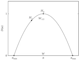
Figure 3 represents the main features of the

multifrac-tal spectrum estimated by the MFDFA method. Here, H0

is the height of the spectrum and represents the most

probable ﬂuctuations in the investigated time scale

boundary of the signal; H2 is the generalized Hurst

expo-nent (also known as correlation degree); αmin represents

behavior of the smallest ﬂuctuations in the spectrum;

αmax represents behavior of the greatest ﬂuctuations in

the spectrum; and W=αmax−αmin is the width of

multi-fractal spectrum that shows the variability of ﬂuctuations

in the spectrum. Multifractal characteristics are quantita-tive measures of the self-similarity and may characterize functional changes in the regulatory processes of the organism. In addition, we also tested the so-called

1/2-width measure of the spectrum, which is deﬁned as

W1/2=∣H2−H0∣ [25]. Table 1 presents summary of all

features used in this study.

2.3. Machine Learning Approaches.For the machine learning

evaluation, the respective functions of the sklearn library

were used [26]. The current paper describes supervised

machine learning methods used. At ﬁrst, the classiﬁers are

trained using a training dataset. For that dataset, the class

labels are known. After that, the eﬃcacy of the classiﬁcation

is evaluated using test set of data. The eﬃcacy is evaluated

by comparing true labels of test set with those predicted by the model.

2.3.1. Discriminant Analysis (DA).In this work, two variants

of the discriminant analysis were tested—linear and

qua-dratic discriminant analyses (LDA and QDA). The LDA aims

to ﬁnd the best linear combination of the input features to

properly separate studied classes. In the case of the QDA, the studied classes are separated by a quadratic function [27].

2.3.2. k-Nearest Neighbors (kNN).Thek-nearest neighbors is one of the nonparametric machine learning approaches. In order to predict the class of the object, method chose the

class, which is the most common among k“neighbors” of

the object. Examples of the“neighbors”are picked from the

training dataset. In the present study, diﬀerent values of the

kare tested—3, 4, and 5 [28].

2.3.3. Support Vector Machine (SVM).The base idea of the support vector machine methods is creation of the

deci-sion hyperplane which would separate diﬀerent classes.

In that case, the margin between two nearest points on

the diﬀerent sides of the hyperplane is maximal. In present

study, the radial basis function (RBF) is used. For

imple-mentation in python, one have to specify the following:

SVC gamma = 2, C = 1 [29].

2.3.4. Decision Trees (DT).The decision trees classiﬁcation model is built around a sequence of the Boolean queries.

The sequence of such queries forms the “trees” structure.

In the present work, variations of the classiﬁer were

analyzed—with ﬁxed value of the maximal tree depth

H

2

H

0

0 1

훼

D

(

훼

)

W

1/2

W

훼_min 훼

max

(6)

(max_depth= 5). The maximal depth feature points the maximal number of queries that is allowed to use before

reaching leaf. The leaf node is the node that has no“

chil-dren” [30].

2.3.5. Naive Bayes (NB).This method is based on the

applica-tion of the Bayes’ theorem with assumptions that data has

strong (or naive) independence. In current study, the Gaussian distribution of data is assumed [31].

2.4. Semioptimal Search of the Noncorrelated Feature Space

2.4.1. Feature Set Selection. In the current investigation, all possible combinations of all features were analyzed. How-ever, it is well known that using combined correlated features

Table_{1: List of studied features.}

Feature Description Equation

M Mean value of the R-R (1)

HR Heart rate (2)

SDNN Standard deviation of the R-R (3)

CV Coeﬃcient of the variation (4)

RMSSD Square root of mean of squares of diﬀerences between successive R-R (5)

NN50 Variation higher than 50 ms in R-R signal —

M₀ Mode of the R-R signal —

VR Variation range of the R-R signal —

AM₀ Amplitude of the mode —

SI Stress index (6)

IAB Index of autonomic balance (7)

ARI Autonomic rhythm index (8)

IARP Index of adequate regulation processes (9)

HF(Fr) High frequency Fourier spectral power —

LF(Fr) Low frequency Fourier spectral power —

VLF(Fr) Very low frequency Fourier spectral power —

TP(Fr) Total power of the Fourier spectrum —

LF/HF(Fr) Autonomic balance exponent of the Fourier spectrum —

HF_max(Fr) Maximum power of the HF —

HFn(Fr), LFn(Fr), and VLFn(Fr) Normalized power of the HF, LF, and VLF Fourier spectrum (10)

IC Index of centralization (11)

IAS Index of the subcortical nervous center’s activation (12)

RF Respiration frequency —

HF(wt) High frequency wavelet spectral power —

LF(wt) Low frequency wavelet spectral power —

VLF(wt) Very low frequency wavelet spectral power —

HF_n(wt), LF_n(wt), and VLF_n(wt) Normalized power of the HF, LF, and VLF wavelet spectrum —

SDHF(wt), SDLF(wt), and SDVLF(wt) Standard deviations of the HF(t), LF(t), and VLF(t) wavelet time series —

TP(wt) Total power of the wavelet spectrum —

LF/HF(wt) Autonomic balance exponent of the wavelet spectrum —

(LF/HF)_max Maximal value of dysfunctions —

(LF/HF)int Intensity of dysfunctions —

Nd Number of dysfunctions —

H Hurst exponent (13)

α_minLF,α_minVLF Smallestﬂuctuations of the LF and VLF spectral band —

α_maxLF,α_maxVLF Greatestﬂuctuations of the LF and VLF spectral band —

WLF, WVLF Spectrum width of the LF and VLF spectral band —

H2LF,H2VLF Correlation degree of the LF and VLF spectral band —

H₀LF,H₀VLF Spectrum height of the LF and VLF spectral band —

(7)

in machine learning may lead to misleading results.

There-fore, theﬁrst step in this investigation is to sort uncorrelated

combinations. For this task, we compute the correlation

coef-ﬁcient. The wholeﬂowchart of the script for noncorrelated

feature combination selection is presented in Figure 4. The threshold correlation value was set to 0.25. Usually, correlation more than 0.75 is considered to be high. There-fore, a value lower than 0.25 is a good benchmark for low

correlation. In the current work, two toﬁve feature

tions were made. In case of more than two feature combina-tions, the correlation was checked pairwise. When all

calculation was ﬁnished, the noncorrelated features were

saved to aﬁle for future purposes.

Table 2 presents the total number ofn-combinations for

53 features in case ofn= [2, 3, 4, 5] and number of selected

noncorrelated combinations. Table 2 shows that application of such selection leads to both, more appropriate results

and signiﬁcant reduction of the analyzed combinations set.

2.4.2. Cross-Validation. Figure 5 presents a complete ﬂ

ow-chart of the implemented algorithm for classiﬁer eﬃcacy

evaluation.

Cross-validation implies division of the original datasets

intomsubsets, whenm-1 subsets are used for the classiﬁer

training. The remaining part is used for the classiﬁer test.

The procedure is repeated m times. Such approach allows

one to use dataset evenly [32].

In the current investigation, the number of random folds l was set to be 5. For the implementation of 5-fold cross-validation, we randomly divide the original dataset into 5 subsets. The division is implemented for both groups simultaneously. As the result, each subset included 6 healthy volunteers and 8 patients diagnosed with hypertension.

Many machine learning methods are sensitive to train

set selection, so, in order to remove such inﬂuence, the

cross-validation procedure was repeated 100 times with

diﬀerent folds. The repeated cross-validation allows to

increase number of classiﬁcation accuracy estimates [33].

Table 3 presents calculation times spent for each

machine learning approach for diﬀerent number of

features in combinations. Calculation times are presented for all noncorrelated combinations. In accordance with

Table 3, the fastest approach is the decision trees. The k

-nearest neighbors approach is the slowest one.

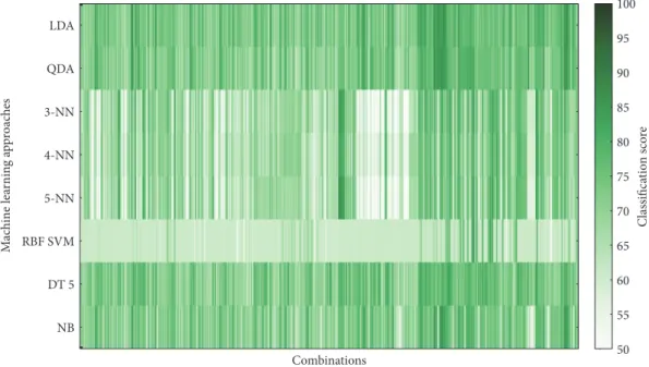
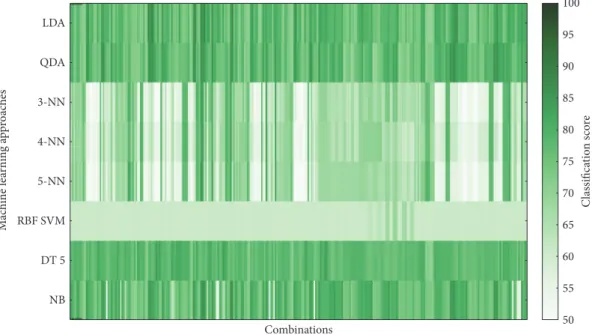
3. Results

The classiﬁer performance was averaged over 5

cross-validations and over 100 implementations. Figures 6–9 show

overview of the classiﬁer performance for all combinations

for diﬀerent numbers of features in combination. All color

bars on Figures 5–8 have the same range—from 50 to 100%.

Figure 10 presents maximal accuracy achieved by each

classiﬁer for diﬀerent number of features in set.

According to the data presented in Figures 5–9, the

highest classiﬁcation is achieved by the discriminant

Start Correlation

evaluation

For each combination

Correlation < 0.25?

End

Save combination Import

dataset

Yes No

All combination studied? Next combination

No

Yes

Figure_{4: Flowchart of the noncorrelated combination selection.}

Table_{2: Noncorrelated combination selection data.}

n

Total

n-combination

number

Selected

n-combinations

Calculation time, sec

2 1378 586 0.027

3 23,426 1669 0.477

4 292,825 1339 11.559

(8)

Start

Import dataset and non-correlated features combinations

For each machine learning approach

For each combination

End

Next machine learning approach Next combination

All combinations studied?

All approaches studied? No

No

Yes

Yes 100 repeated

5-fold cross-validation

Figure_{5: Flowchart of classi}_ﬁ_{er e}_ﬃ_{cacy evaluation algorithm.}

Table_{3: Calculation times of classi}_ﬁ_{er e}_ﬃ_{cacy evaluation, sec.}

Features in combinations LDA QDA NN3 NN4 NN5 RBF SVM DT Naive Bayes

2 165 113 281 281 281 139 89 130

3 482 346 917 860 806 403 269 375

4 397 288 640 643 642 325 222 300

5 88 64 141 140 140 71 50 66

LDA

QDA

3-NN

4-NN

5-NN

RBF SVM

DT 5

NB

M

ac

hine le

ar

nin

g a

p

roac

h

es

Combinations

100

95

90

85

80

75

70

65

60

55

50

C

lassifica

tio

n s

co

re

(9)

analysis. Moreover, in Figures 5–8, it can be clearly seen that approaches of discriminant analysis have more com-binations with relatively high score than any other approach. Furthermore, for the support vector machine

approach, only few combinations have acceptable classiﬁ

-cation score level.

It is worthy to mention that generally classiﬁcation

accuracy rises as the number of features in the feature set increases. For 4-feature sets, the maximum is

achieve-d—accuracy for 5-feature sets is lower for all machine

learning approaches. It drops signiﬁcantly in case of

sup-port vector machine approach.

Table 4 presents best results achieved by all machine learning approaches for 4-feature set.

Data in Table 4 shows that linear and quadratic DA not

only achieve higher classiﬁcation score but also have better

stability of the results. Naïve Bayes classiﬁer also has

rela-tively high classiﬁcation score and low deviation.

Among 53 studied features, 36 form combinations that

have the classiﬁcation score higher than 85. Table 5 presents

LDA

QDA

3-NN

4-NN

5-NN

RBF SVM

DT 5

NB

M

ac

hine le

ar

nin

g a

p

roac

h

es

Combinations

100

95

90

85

80

75

70

65

60

55

50

C

lassifica

tio

n s

co

re

Figure_{7: Classi}_ﬁ_{er score for 3-feature combinations.}

LDA

QDA

3-NN

4-NN

5-NN

RBF SVM

DT 5

NB

M

ac

hine le

ar

nin

g a

p

roac

h

es

Combinations

100

95

90

85

80

75

70

65

60

55

50

C

lassifica

tio

n s

co

re

(10)

occurrences of the features among the combinations. The

highest occurrences are noted for diﬀerent spectral features,

associated with VLF spectral band, LF/HF ratio, and statisti-cal feature heart rate.

Table 6 presents 7 features that form combinations with accuracy higher than 90%. All these combinations consist of heart rate, one feature associated with LF/HF ratio, and two features associated with VLF spectral band.

4. Discussion

For discussion purposes, a comparison of the results of the current study with results of one of the commonly used pro-cedure, principal components analysis (PCA), was executed.

The PCA is a statistical procedure used to reveal the internal

structure of the dataset [34]. In our case, features of diﬀerent

amplitude are used; PCA is known to be sensitive to the rel-ative scaling of the feature dataset. Therefore, prior to the PCA application, the standardization procedure was

imple-mented for each of 53 diﬀerent features—subtraction of the

mean value and after that division by the standard deviation. Table 7 presents explained variance as well as the

cumu-lative variance for theﬁrst 15 principal components. First 10

principal components explain 93% of the variance. Conse-quent principal components add 1% of the variance or less.

In order to compare results of the semioptimal search of the noncorrelated feature space with PCA, combinations of

the ﬁrst 10 components were consequently tested for all

LDA

QDA

3-NN

4-NN

5-NN

RBF SVM

DT 5

NB

M

ac

hine le

ar

nin

g a

p

roac

h

es

Combinations

100

95

90

85

80

75

70

65

60

55

50

C

lassifica

tio

n s

co

re

Figure_{9: Classi}_ﬁ_{er score for 5-feature combinations.}

85.1% 85.6% 85.9% 85.6% 87.6% 87.8% 84.3% 83.8%

88.7% 88.6% 87.5% 85.5% 87.1% 87.5% 85.0% 88.2%

91.3% 90.3% 87.1% 85.6% 86.6% 86.7% 87.1% 88.2%

89.1% 87.4% 85.1% 84.2% 86.5% 69.3% 84.4% 86.1% 2

3

4

5

N

um

b

er o

f f

ea

tur

es in s

et

LDA QDA 3-NN 4-NN 5-NN RBF SVM DT 5 NB

Classifier

(11)

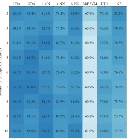
machine learning approaches using 100 repeated 5-fold cross-validation. Figure 11 presents the maximal results of

classiﬁcation accuracy achieved by each machine learning

approach using combinations of the principal components. Comparing the results of Figures 10 and 11, one can note that features found by the semioptimal search of

the noncorrelated feature space reach higher classiﬁcation

accuracies than combinations of the principal components for all tested machine learning approaches.

5. Conclusions

In this work, various machine learning approaches were tested in task of the arterial hypertension diagnostics. In earlier works, the same datasets were used for investigation of the linear and quadratic DA methods [11]. The present work implies comparison of the DA methods with other machine learning approaches, like support vector machine,

k-nearest neighbors, Naive Bayes, and decision trees.

The results of the current investigation showed that for the studied task, the application of the discriminant

Table_{4: Best classi}_ﬁ_{cation scores.}

Score, % Features

Linear discriminant analysis

91.33±1.75 HR VLFn(Fr) LF/HF(Fr) VLF(wt)

90.30±1.37 HR VLF_n(Fr) VLF(wt) (LF/HF)_int

90.04±1.85 HR LF/HF(Fr) VLF(wt) VLFn(wt)

90.44±1.60 HR VLF_n(Fr) LF/HF(Fr) SDVLF

90.11±1.80 HR LF/HF(Fr) SDVLF VLFn(wt)

90.16±1.61 HR SDVLF VLF_n(wt) (LF/HF)_int

Quadratic discriminant analysis

90.31±1.71 HR VLF_n(Fr) LF/HF(Fr) VLF(wt)

3-nearest neighbors

87.14±2.12 LF/HF(Fr) SDVLF VLF_n(wt) W_1/2VLF

4-nearest neighbors

85.56±2.40 SDVLF VLF_n(wt) LF/HF(wt) W_1/2VLF

5-nearest neighbors

86.63±1.30 HR HF(Fr) LF_n(Fr) W_1/2VLF

Support vector machine, radial base function

86.73±2.24 IAS RF a₂LF WVLF

Decision trees, max depth 5

87.10±3.40 IARP LF/HF(Fr) IAS WLF

Decision trees, no max depth

87.34±3.08 IARP LF/HF(Fr) IAS WLF

Naïve Bayes classiﬁer

88.17±1.07 VLF(Fr) VLF_n(Fr) LF/HF(Fr) W_1/2LF

Table _{5: Features occurrences for classi}_ﬁ_{cation score higher}

than 85%.

Features Occurrences, % Features Occurrences, %

VLF_n(Fr) 50.89 Nd 4.73

VLF(Fr) 50.89 M0 4.73

VLF_n(wt) 47.93 WLF 4.73

W1/2VLF 34.91 IARP 3.55

LF/HF(Fr) 34.32 IC 2.96

HR 33.73 HF(Fr) 2.96

SDVLF 30.18 α₂LF 2.96

(LF/HF)max 24.26 LFn(wt) 2.37

LF/HF(wt) 18.34 SI 2.37

(LF/HF)int 18.34 LFn(Fr) 1.78

W_1/2LF 17.75 α_minLF 1.78

H 13.61 ARI 1.78

WVLF 13.02 HF_n(Fr) 1.78

IAS 10.65 SDHF 1.18

VLF(wt) 7.69 IAB 0.59

RF 6.51 NN50 0.59

α_maxLF 5.92 α₀LF 0.59

M 5.33 αmaxVLF 0.59

Table _{6: Feature occurrences for classi}_ﬁ_{cation score higher}

than 90%.

Features Occurrences, %

HR 100.00

LF/HF(Fr) 62.50

VLF(wt) 62.50

VLFn(wt) 50.00

VLF_n(Fr) 50.00

SDVLF 37.50

(LF/HF)_int 37.50

Table_{7: Dataset analysis by PCA.}

Principal component

Explained variance, %

Cumulative variance, %

1 34.88 34.88

2 17.65 52.54

3 13.03 65.57

4 8.87 74.45

5 5.38 79.83

6 4.10 83.93

7 3.55 87.47

8 2.42 89.89

9 1.78 91.67

10 1.36 93.03

11 1.01 94.04

12 0.95 94.98

13 0.84 95.82

14 0.74 96.56

(12)

analysis (linear and quadratic) revealed to be the most

appropriate classiﬁers. These approaches have high classiﬁ

-cation score and low deviations over diﬀerent realizations.

A set of four features in combination seems to be the

opti-mal number, as the classiﬁcation accuracy score is higher

and more consistent than those for two, three, and ﬁve

features in combination.

Prevalence of the VLF and LF/HF spectral features among best combinations might indicate that sympathetic nervous system takes an important part in the initialization of the arterial hypertension and maintenance of the increased vascular tone as well as increased cardiac output. These

results are in accordance with scientists’ interpretation of

the arterial hypertension development [35, 36].

The results of the suggested approach were compared with data set prepared by the commonly used procedure of

principal component analysis. Results of the n-feature

noncorrelated sets have achieved higher classiﬁcation

accu-racies than ones based on the dataset of the selected prin-cipal components.

In future works, our research group will continue to improve results on this problem. One of the investiga-tions that are planned is to analyze robustness of the

classiﬁers based on multiple signals recorded

simulta-neously. Among the other perspective directions of future investigation is usage of the advanced neural net-works [37] and genetic algorithms [38] for feature

extraction and classiﬁcation.

Conflicts of Interest

The authors declare that there are no conﬂicts of interest

regarding the publication of this paper.

Acknowledgments

The work was supported by the Act 211 Government of the Russian Federation, Contract no. 02.A03.21.0006, and by the FCT project AHA CMUP-ERI/HCI/0046/2013.

References

[1] T. Rosenthal and A. Alter,“Occupational stress and

hyperten-sion,”Journal of the American Society of Hypertension, vol. 6,

no. 1, pp. 2–22, 2012.

[2] X. L. Feng, M. Pang, and J. Beard,“Health system

strengthen-ing and hypertension awareness, treatment and control: data

from the China health and retirement longitudinal study,”

Bulletin of the World Health Organization, vol. 92, no. 1,

pp. 29–41, 2014.

[3] M. V. Kamath, M. Watanabe, and A. Upton, Heart Rate

Variability (HRV) Signal Analysis: Clinical Applications, CRC Press, New York, 2012.

[4] I. B. Ushakov, O. I. Orlov, R. M. Baevskii, E. Y. Bersenev, and

A. G. Chernikova, “Conception of health: space-earth,”

Human Physiology, vol. 39, no. 2, pp. 115–118, 2013.

[5] P. Melillo, M. Bracale, and L. Pecchia,“Nonlinear heart rate

variability features for real-life stress detection. Case study:

82.4% 81.4% 81.6% 78.2% 82.9% 67.6% 77.4% 82.2%

80.2% 81.5% 82.5% 77.2% 82.5% 63.6% 76.3% 79.9%

81.1% 83.1% 84.9% 80.7% 80.3% 60.8% 77.7% 78.8%

83.2% 85.5% 81.8% 78.2% 80.5% 60.9% 76.0% 78.6%

84.0% 84.5% 82.3% 79.6% 80.2% 60.9% 76.0% 76.8%

85.3% 85.0% 82.5% 78.6% 80.7% 60.9% 79.2% 76.2%

84.4% 82.8% 84.4% 80.9% 81.8% 60.9% 77.6% 75.7%

83.6% 81.1% 84.0% 80.2% 81.5% 60.8% 77.8% 73.3%

82.7% 81.9% 84.7% 80.0% 83.4% 61.0% 78.0% 74.0% 2

3

4

5

6

7

8

9

10

N

um

b

er o

f p

rinci

pal co

m

p

o

n

en

ts

LDA QDA 3-NN 4-NN 5-NN RBF SVM DT 5 NB

(13)

students under stress due to university examination,” Biomed-ical Engineering Online, vol. 10, no. 96, pp. 1–13, 2011. [6] F. Ebrahimi, S. K. Setarehdan, J. Ayala-Moyeda, and H.

Nazeran, “Automatic sleep staging using empirical mode

decomposition, discrete wavelet transform, time-domain, and

nonlinear dynamics features of heart rate variability signals,”

Computer Methods and Programs in Biomedicine, vol. 112,

no. 1, pp. 47–57, 2013.

[7] A. H. Khandoker, M. Palaniswami, and C. K. Karmakar,

“Support vector machines for automated recognition of

obstructive sleep apnea syndrome from ECG recordings,”

IEEE Transactions on Information Technology in Biomedicine,

vol. 13, no. 1, pp. 37–48, 2009.

[8] U. Parlitz, S. Berg, S. Luther, A. Schirdewan, J. Kurths, and N.

Wessel,“Classifying cardiac biosignals using ordinal pattern

statistics and symbolic dynamics,”Computers in Biology and

Medicine, vol. 42, no. 3, pp. 319–327, 2012.

[9] M. O. Mendez, J. Corthout, S. Van Huﬀel et al.,“Automatic

screening of obstructive sleep apnea from the ECG based on

empirical mode decomposition and wavelet analysis,”

Physio-logical Measurement, vol. 31, no. 3, pp. 273–289, 2010.

[10] V. Kublanov, A. Dolganov, and V. Borisov,“Application of

the discriminant analysis for diagnostics of the arterial hypertension - analysis of short-term heart rate variability

signals,” in presented at the 4th International Congress on

Neurotechnology, Electronics and Informatics, pp. 45–52, 2016.

[11] V. Kublanov, A. Dolganov, and Y. Kazakov,“Diagnostics of

the arterial hypertension by means of the discriminant analysis - analysis of the heart rate variability signals features

combina-tions,”inpresented at the BIOSTEC 2017 - Special Session on

Neuro-electrostimulation in Neurorehabilitation Tasks,

pp. 291–298, 2017.

[12] M. Malik,“Heart rate variability: standards of measurement,

physiological interpretation, and clinical use,” Circulation,

vol. 93, no. 5, pp. 1043–1065, 1996.

[13] R. M. Baevskiy,“Аnaliz variabelnosti serdechnogo ritma pri

ispolzovanii razlichnykh ehlektrokardiograﬁcheskikh sistem

(metodicheskie rekomendatsii) [Analysis of heart rate

variabil-ity using diﬀerent electrocardiographic systems (guidelines)],”

Vestnik aritmologii [Herald Arhythmology], no. 24, pp. 65–87, 2001.

[14] F. A. Jain, I. A. Cook, A. F. Leuchter et al.,“Heart rate

variabil-ity and treatment outcome in major depression: a pilot study,”

International Journal of Psychophysiology, vol. 93, no. 2,

pp. 204–210, 2014.

[15] N. B. Haspekova, “Diagnosticheskaya informativnost

monitorirovaniya variabelnosti serdechnogo ritma serdca [Diagnostic Informativeness of the heart rate variability

monitoring],” Vestnik aritmologii [Herald Arhythmology],

vol. 32, pp. 15–23, 2003.

[16] M. Adnane, Z. Jiang, and Z. Yan,“Sleep–wake stages

classi-ﬁcation and sleep eﬃciency estimation using single-lead

electrocardiogram,”Expert Systems with Applications, vol. 39,

no. 1, pp. 1401–1413, 2012.

[17] P. S. Addison,“Wavelet transforms and the ECG: a review,”

Physiological Measurement, vol. 26, no. 5, pp. R155–R199, 2005.

[18] S. Mallat,A Wavelet Tour of Signal Processing, 2009.

[19] V. S. Kublanov,“A hardware-software system for diagnosis

and correction of autonomic dysfunctions,” Biomedical

Engineering, vol. 42, no. 4, pp. 206–212, 2008.

[20] D. Rubin, T. Fekete, and L. R. Mujica-Parodi, “Optimizing

complexity measures for fMRI data: algorithm, artifact, and

sensitivity,”PloS One, vol. 8, no. 5, 2013.

[21] B. B. Mandelbrot,“Multifractal power law distributions:

nega-tive and critical dimensions and other“anomalies,”explained

by a simple example,”Journal of Statistical Physics, vol. 110,

no. 3–6, pp. 739–774, 2003.

[22] H. E. Stanley, L. A. N. Amaral, A. L. Goldberger, S. Havlin, P.

C. Ivanov, and C.-K. Peng,“Statistical physics and physiology:

monofractal and multifractal approaches,”Physica A:

Statisti-cal Mechanics and its Applications, vol. 270, no. 1-2, pp. 309– 324, 1999.

[23] E. A. F. Ihlen, “Introduction to multifractal detrended

ﬂuctuation analysis in Matlab,” Frontiers in Physiology,

vol. 3, pp. 141–150, 2012.

[24] D. Makowiec, A. Rynkiewicz, J. Wdowczyk-Szulc, and M.

Zarczynska-Buchowiecka, “On reading multifractal spectra.

Multifractal age for healthy aging humans by analysis of

cardiac interbeat time intervals,” Acta Physica Polonica B

Proceedings Supplement, vol. 5, no. 1, pp. 159–170, 2012.

[25] D. Makowiec, A. Rynkiewicz, R. Gałaska, J. Wdowczyk-Szulc,

and M. Żarczyńska-Buchowiecka, “Reading multifractal

spectra: aging by multifractal analysis of heart rate,” EPL

Europhysics Letters, vol. 94, no. 6, p. 68005, 2011.

[26] F. Pedregosa, G. Varoquaux, A. Gramfort et al.,“Scikit-learn:

machine learning in python,” Journal of Machine Learning

Research, vol. 12, pp. 2825–2830, 2011.

[27] G. McLachlan,Discriminant Analysis and Statistical Pattern

Recognition, vol. 544, John Wiley & Sons, 2004.

[28] L. E. Peterson, “K-nearest neighbor,” Scholarpedia, vol. 4,

no. 2, p. 1883, 2009.

[29] J. A. Suykens and J. Vandewalle,“Least squares support vector

machine classiﬁers,”Neural Processing Letters, vol. 9, no. 3,

pp. 293–300, 1999.

[30] P. H. Swain and H. Hauska, “The decision tree classiﬁer:

design and potential,” IEEE Transactions on Geoscience

Electronics, vol. 15, no. 3, pp. 142–147, 1977.

[31] K. P. Murphy, Naive Bayes Classiﬁers, Univ. Br, Columbia,

2006.

[32] R. Kohavi,“A study of cross-validation and bootstrap for

accu-racy estimation and model selection,”Ijcai, vol. 14, pp. 1137–

1145, 1995.

[33] P. Refaeilzadeh, L. Tang, and H. Liu, “Cross-validation,” in

Encyclopedia of Database Systems, pp. 532–538, Springer, 2009.

[34] I. Jolliﬀe,Principal Component Analysis, Wiley Online Library,

2002.

[35] G. Parati and M. Esler,“The human sympathetic nervous

sys-tem: its relevance in hypertension and heart failure,”European

Heart Journal, vol. 33, no. 9, pp. 1058–1066, 2012.

[36] G. Mancia, R. Fagard, K. Narkiewicz et al.,“2013 ESH/ESC

guidelines for the management of arterial hypertension,”

Euro-pean Heart Journal, vol. 34, no. 28, pp. 2159–2219, 2013. [37] H. B. Demuth, M. H. Beale, O. De Jess, and M. T. Hagan,

Neural network design, Martin Hagan, 2014.

[38] A. Fraser and D. Burnell, Computer Models in Genetics,

(14)

,QWHUQDWLRQDO-RXUQDORI

$HURVSDFH

(QJLQHHULQJ

+LQGDZL3XEOLVKLQJ&RUSRUDWLRQ

KWWSZZZKLQGDZLFRP 9ROXPH

Robotics

Journal of

Hindawi Publishing Corporation

http://www.hindawi.com Volume 2014

Active and Passive Electronic Components

Control Science and Engineering Journal of

Machinery

Hindawi Publishing Corporation http://www.hindawi.com

Journal of

(QJLQHHULQJ

Volume 201

Submit your manuscripts at

https://www.hindawi.com

VLSI Design

Hindawi Publishing Corporation

http://www.hindawi.com Volume 201

-Hindawi Publishing Corporation

Shock and Vibration

Civil Engineering

Advances in

Acoustics and VibrationAdvances in

http://www.hindawi.com Volume 2014 Hindawi Publishing Corporation

Electrical and Computer Engineering

Journal of

Advances in OptoElectronics

The Scientific

World Journal

Sensors

Journal of

Modelling & Simulation in Engineering

Chemical Engineering

International Journal of Antennas and

Propagation International Journal of

Navigation and Observation International Journal of

Distributed Sensor Networks