Journal of Geophysical Research: Biogeosciences

Climate change impacts on the vegetation carbon

cycle of the Iberian Peninsula

_—

Intercomparison

of CMIP5 results

Sara Aparício1, Nuno Carvalhais1,2, and Júlia Seixas1

1_{Center for Environmental and Sustainability Research, Departamento de Ciências e Engenharia do Ambiente, Faculdade de} Ciências e Tecnologia, Universidade Nova de Lisboa, Caparica, Portugal,2_{Max Plank Institute for Biogeochemistry, Jena, Germany}

Abstract

The vulnerability of a water-limited region like the Iberian Peninsula (IP) to climate changes drives a great concern and interest in understanding its impacts on the carbon cycle, namely, in terms of biomass production. This study assesses the effects of climate change and rising CO2on forest growth, carbon sequestration, and water-use efficiency on the IP by late 21st century using 12 models from the CMIP5 project (Coupled Model Intercomparison Project Phase 5). Wefind a strong agreement among the models under representative concentration pathway 4.5 (RCP4.5) scenario, mostly regarding projected forest growth and increased primary production (13, 9% of gross primary production (GPP) increase projected by the models ensemble). Under RCP8.5 scenario, the results are less conclusive, as seven models project both GPP and net primary production to increase (up to 83% and 69%, respectively), while the remaining four models project the IP as a potential carbon source by late century. Divergences in carbon mass in wood predictions could be attributed to model structures, such as the N cycle, land model component, land cover data and parameterization, and distinct clusters of Earth System Models (ESMs). ESMs divergences in carbon feedbacks are likely being highly impacted by parameterization divergences and susceptibility to climate change and CO2 fertilization effect. Despite projected rainfall reductions, we observe a strong agreement between models regarding the increase of water-use efficiency (by 21% and 34%) under RCP4.5 and RCP8.5, respectively. Results suggest that rising CO2has the potential to partially alleviate the adverse effects of drought.

1. Introduction

Predicted changes in climate conditions and land use are likely to have significant effects on ecosystem services, namely, on biomass production for energy use. The consistently projected increases in temperature (by +5.5°C) and decreases in precipitation (by 30%) by the end of the century for the Mediterranean basin [Kelemen et al., 2009] may have a large impact on forests and the related ecosystem services they provide [Keenan et al., 2011]. As such, the Mediterranean region is being considered one of the most vulnerable climatic change hot spots [Giorgi, 2006;Benoit and Comeau, 2005;Giorgi and Lionello, 2008], with projected particularly intense land-atmosphere feedbacks [Seufert et al., 1995], mainly due to expected water resources scarcity [Benoit and Comeau, 2005].

In semiarid ecosystems, as is the case of most of the Iberian Peninsula (IP), ecosystems are water limited, meaning that productivity is broadly controlled by water availability [Reichstein et al., 2002]. Henceforth, the ecosystem services and goods in the IP are under a growing threat by the observed decreasing trend of annual precipitation (in addition to variations in temperature,fire regimes, and other human influences) [Montaldo et al., 2008;Lindner et al., 2010]. Also, carbon sequestration potential will be impacted by more frequent droughts [Tubiello et al., 2007;Frank et al., 2013].Ciscar et al. [2011] predicted that Southern Europe would experience the largest yield losses, which would reach approximately 25% by 2080 under a 5.4°C temperature increase. Recent events, such as the intense drought throughout the Iberian Peninsula in 2004/2005, resulted in significant cereals production reduction of ~40% on average [García-Herrera et al., 2007]. Also, deciduous broadleaf forests (beech and oaks) in northern central Italy, which is partly characterized by a Mediterranean climate [Kottek et al., 2006]), showed reductions in growth rate up to 50% in 2000–2004 compared to those in 1997–1999, due to a marked water deficit [Bertini et al., 2011]. However, some experiments and yield surveys suggest that forest productivity will be positively impacted by warming temperatures [Keenan et al., 2011], as the result of the direct fertilization effect of increased CO2, besides other indirect effects, is the lengthening of

PUBLICATIONS

Journal of Geophysical Research: Biogeosciences

RESEARCH ARTICLE

10.1002/2014JG002755

Key Points:

•Forest growth and GPP increase are simulated under RCP4.5 scenario •RCP8.5 results are less conclusive as

projections vary considerably among models

•Most models project increase of water-use efficiency as CO2rises

Correspondence to:

S. Aparício,

s.aparicio@campus.fct.unl.pt

Citation:

Aparício, S., N. Carvalhais, and J. Seixas (2015), Climate change impacts on the vegetation carbon cycle of the Iberian Peninsula—Intercomparison of CMIP5 results,J. Geophys. Res. Biogeosci.,120, 641–660, doi:10.1002/2014JG002755.

Received 31 JUL 2014 Accepted 25 FEB 2015

the growing season. These contradictory results indicate that elevated CO2concentration ([CO2]) may offset negative impacts that climate change may have on productivity. For example,Norby et al. [2005] suggest that the growth response of trees to elevated CO2is relatively predictable across a broad range of sites, with an average increase of 23% when doubling the CO2levels up to 550 ppm.Gaucherel et al. [2008] project a significant increase in productivity of pine and oak (+26 and +43%, respectively) by the end of the 21st century, due to the direct effect of CO2increase. One reason refers to the fact that plants are able to increase their water-use efficiency (WUE), an important characteristic of ecosystem productivity linking carbon and water cycling [Prior et al., 2011], implying an enhanced resistance of vegetation to drought.

Earth System Models (ESMs) are used to project trends in vegetation productivity and carbon storage. They incorporate components describing the atmosphere’s interaction with land use and vegetation, while taking into account atmospheric chemistry, aerosols, and the carbon cycle [Taylor et al., 2012]. ESMs may differ in its parameterization and forcing components (i.e., change in climate and atmospheric [CO2]) leading to contradictory answers to the same questions [Friedlingstein et al., 2006], contributing to uncertainties in terrestrial sources and sinks of CO2. The wide range of published estimates, from dynamic global vegetation models (DGVMs; [Sitch et al., 2008]) and ESMs [Friedlingstein et al., 2006], differs in their projections due to different but plausible representations of the underlying processes [Ahlström et al., 2012]. Despite the vast improvement of models in the last decades, some challenging uncertainties remain, preventing the prediction of accurate long-term impacts of climate on the forestry sector. Therefore, it is of high interest to get a better understanding of the response of the terrestrial biosphere to slender the large models uncertainty.

In this study, we assess the results from 12 models from the Coupled Model Intercomparison Project Phase 5 (CMIP5) exercise [Taylor et al., 2012] regarding the carbon balance projected for the Iberian Peninsula. The following variables are considered: carbon mass in wood (Cwood), carbon in vegetation (Cveg), gross primary production (GPP), and net primary production (NPP). We aim to better understand the modeled effects of changing climate on vegetation activity by analyzing multiple drivers of climate change, namely, precipitation, air surface temperature, and atmospheric [CO2]. A particular focus on how models accommodate WUE is undertaken, since precipitation is projected to decline, in order to diagnose how models simulate the response of carbonfluxes to water stress. Model intercomparison analysis of Cwood is expected to provide different responses of IP’s forest growth and carbon accumulation in relation to current climate. In order to understand the modeled impact of increasing atmospheric [CO2] we consider two climate scenarios: one accounting for the impacts of climate changes and elevated CO2, and the other accounting solely for the effect of CO2. In section 2 we describe the study area and methodology, in section 3 we disclose the main results, and in section 4 we discuss trends, drivers of feedbacks, and sources of uncertainties. Finally, in section 5 we present the main conclusions. The results and discussion follows a three-component framework for intercomparing the 12 CMIP5 models: (1) trends of carbonfluxes and storage for different climate change projections, (2) sensitivity of carbonfluxes to climate variables, and (3) changes in water-use efficiency associated to increases in water scarcity.

2. Materials and Methods

2.1. CMIP5 Models Description and Experiment Design

We use data from 12 ESMs from thefifth phase of the Coupled Model Intercomparison Project (CMIP5) listed in Table 1 and obtained from the Earth System Grid Federation (ESGF) gateways of the Program for Climate Model Diagnosis and Intercomparison (PCMDI) (http://pcmdi9.llnl.gov/esgf-web-fe/), and the Norwegian Storage Infrastructure project (NorStore) (http://noresg.norstore.no/esgf-web-fe/).

The 12 ESMs were selected based on the following requirements: (i) data should be available for the 30 year periods corresponding to the historical period (set as reference scenario) and to the future scenarios period; (ii) data should be available for the four carbon variables of interest (namely, NPP, GPP, Cwood, and Cveg); and for precipitation, air surface temperature, and evapotranspiration; (iii) temporal resolution for each model and variable should be monthly. All models represent vegetation as a mixture of plant functional types (PFTs) that may vary in response to variations in climate and [CO2] forcing. Some models also simulate dynamic vegetation explicitly (by describing mortality, establishment, and succession) whose differences will be taken in consideration.

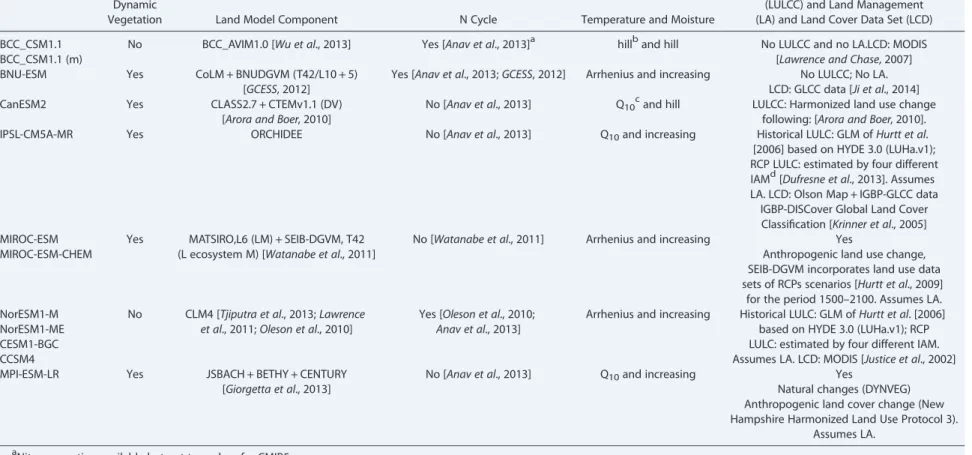
Table 1. Models Used in This Study

Dynamic

Vegetation Land Model Component N Cycle Temperature and Moisture

Land use Land Cover Change (LULCC) and Land Management (LA) and Land Cover Data Set (LCD)

BCC_CSM1.1 No BCC_AVIM1.0 [Wu et al., 2013] Yes [Anav et al., 2013]a hillband hill No LULCC and no LA.LCD: MODIS [Lawrence and Chase, 2007] BCC_CSM1.1 (m)

BNU-ESM Yes CoLM + BNUDGVM (T42/L10 + 5) [GCESS, 2012]

Yes [Anav et al., 2013;GCESS, 2012] Arrhenius and increasing No LULCC; No LA. LCD: GLCC data [Ji et al., 2014]

CanESM2 Yes CLASS2.7 + CTEMv1.1 (DV)

[Arora and Boer, 2010]

No [Anav et al., 2013] Q10cand hill LULCC: Harmonized land use change following: [Arora and Boer, 2010]. IPSL-CM5A-MR Yes ORCHIDEE No [Anav et al., 2013] Q10and increasing Historical LULC: GLM ofHurtt et al. [2006] based on HYDE 3.0 (LUHa.v1); RCP LULC: estimated by four different IAMd[Dufresne et al., 2013]. Assumes LA. LCD: Olson Map + IGBP-GLCC data

IGBP-DISCover Global Land Cover Classification [Krinner et al., 2005] MIROC-ESM Yes MATSIRO,L6 (LM) + SEIB-DGVM, T42

(L ecosystem M) [Watanabe et al., 2011]

No [Watanabe et al., 2011] Arrhenius and increasing Yes

MIROC-ESM-CHEM Anthropogenic land use change,

SEIB-DGVM incorporates land use data sets of RCPs scenarios [Hurtt et al., 2009]

for the period 1500–2100. Assumes LA. NorESM1-M No CLM4 [Tjiputra et al., 2013;Lawrence

et al., 2011;Oleson et al., 2010]

Yes [Oleson et al., 2010;

Anav et al., 2013]

Arrhenius and increasing Historical LULC: GLM ofHurtt et al. [2006] based on HYDE 3.0 (LUHa.v1); RCP LULC: estimated by four different IAM. Assumes LA. LCD: MODIS [Justice et al., 2002] NorESM1-ME

CESM1-BGC CCSM4

MPI-ESM-LR Yes JSBACH + BETHY + CENTURY [Giorgetta et al., 2013]

No [Anav et al., 2013] Q10and increasing Yes

Natural changes (DYNVEG) Anthropogenic land cover change (New Hampshire Harmonized Land Use Protocol 3).

Assumes LA. a_{Nitrogen option available but not turned on for CMIP5 run.}

b_{Function that increases to a maximum and then decreases.} c_Q

10value dependent on temperature.

d_{Integrated Assessment Modelling (IAM) groups provided the CMIP5 community with four representative concentration pathways (RCPs) of greenhouse gases, aerosols, and land use and land}

cover changes through the 21st century [Brovkin et al., 2013].

Journal

of

Geophysical

Research:

Biogeosciences

10.1002/

2014JG002755

AP

ARÍCIO

ET

AL.

©2015.

American

Geoph

ysical

Union.

All

Rights

Rese

rved.

Two representative concentration pathways (RCPs) [Moss et al., 2010] were retained for analysis, namely, RCP4.5 and RCP8.5, also used for the CMIP5 project. These two scenarios reflect global GPP, NPP, and Cwood responses to CO2increase and climate change simultaneously. Data were not available for the variable Cwood for MPI-ESM-LR and the variable evapotranspiration for CCSM4 model under the RCP8.5 scenario.

Afixed climate scenario assuming the CO2from RCP4.5 scenario (“esmFixClim2”experiment) was also retained. This scenario suppresses changes in climate forcing that respond to CO2in order to assess changes in NPP, GPP, and Cwood considering only CO2increase. Only the models BCC_CSM1.1, CanESM2, and MIROC-ESM had GPP, NPP, and Cwood data available of the FixClim experiment.

2.2. Study Area

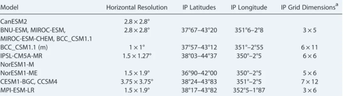
The Iberian Peninsula (IP) is located in southwestern Europe (roughly 37°1′N to 43°20′N, and 350°20′E to 2°20′E). It comprises approximately 20% of the surface area of the Mediterranean region [Quézel, 1985] and crosses three main types of climates: Mediterranean climate, oceanic climate, and semiarid climate [Kottek et al., 2006]. Spatial ranges and sample dimension per model differ slightly between models, since they have different resolutions. Table 2 presents the selection of area for each model based on the coordinates of the actual IP.

2.3. Data Processing

We used 30 year periods to construct a representative climatology of historical and future climate and ecosystem responses to climate variability. Historical period refers to 1970 to 1999, while future projections refer to a 100 year span from the historical period. We consider the period between 2070 and 2099 for data analysis.

2.3.1. Model Output

Our analysis is based on the evaluation of mean annualfields of climate and response variables as outputted by the models. The changes between the historical period and future scenarios are obtained by computing the relative differences (%) of the variable of interest (X), e.g.,

ΔXRCP4:5 Histo¼

XRCP4:5 XHisto

XHisto

100 (1)

As an example, in order to compute the relative change of mean annual NPP in the Iberian Peninsula under the climate projection RCP4.5 in comparison to the historical period (ΔNPPRCP4.5-Histo), the mean annual NPP over each grid pixel was averaged by 30 years for both historical and RCP4.5 scenarios (NPPHISTOand NPPRCP45, respectively) and quantified as follows:

ΔNPPRCP4:5 Histo¼

NPPRCP4:5 NPPHisto

NPPHisto

100 (2)

A matrix with spatial representation of mean NPP relative changes is generated as output. Afterward, the whole grid is spatially averaged generating the value of the overall change for the study area.

2.3.2. Impact of CO2Fertilization and Climate Change CO2Driven on Carbon Fluxes

The FixClim experiments, which assumes the same concentrations of atmospheric CO2as in the RCP4.5 experiment, were used to assess the effect of climate change on carbonfluxes, when climate change that

Table 2. Iberian Peninsula (IP) Coordinates Selection for Each Model

Model Horizontal Resolution IP Latitudes IP Longitude IP Grid Dimensionsa

CanESM2 2.8 × 2.8°

BNU-ESM, MIROC-ESM, MIROC-ESM-CHEM, BCC_CSM1.1

2.8 × 2.8° 37°67–43°20 351°6–2°8 3 × 5

BCC_CSM1.1 (m) 1 × 1° 37°57–43°12 351°–2°55 6 × 11

IPSL-CM5A-MR 1.5 × 1.27° 38°03–44°37 350°–2°5 6 × 6

NorESM1-M

NorESM1-ME 1.5 × 1.9° 36°90–42°00 350°–2°5 5 × 6

CESM1-BGC, CCSM4 3.75 × 3.75° 38°24–43°83 351°–2°5 7 × 12

MPI-ESM-LR 1.5 × 1.9° 38°17–43°82 352°5–1°87 3 × 6

a_{Number of pixels of each matrix representing the IP.}

should respond to CO2increase was suppressed. Equation (3) indicates the change of NPP relative to historic period (ΔNPPFixClim-Histo), as a response to the sole effect of CO2while climate change resulting from increasing CO2is neglected.

ΔNPPFixClim Histo¼NPPFixClim NPPHisto

NPPHisto

100 (3)

Combining FixClim with the RCP4.5 experiment enables to reflect how carbon cycle is affected by climate change under conditions of increasing CO2. This is formulated as follows:

δNPPFixClim RCP4:5¼NPPFixClim NPPRCP4:5 (4)

ΔNPPFixClim

RCP4:5 ¼

δNPPFixClim RCP4:5

NPPRCP45

100 (5)

whereδNPPFixClim-RCP4.5indicates the change of NPP due to climate change andΔNPPFixClimRCP4:5the relative

changes due to climate change, when both climate change and CO2fertilization are considered. 2.3.3. Response of Carbon Variables and Water-Use Efficiency to Climate Variables

The assessment of the response of carbon variables to changing climate variables (i.e., variation of carbonflux per unit of change of climate variable) was obtained through the ratio between the differences between future and historical means of each variable, expressed as follows:

δNPPRCP4:5 Histo¼NPPRCP4:5 NPPHisto (6)

δET4:5 Histo¼ETRCP4:5 ETHisto (7)

ρNPPET¼δNPPRCP4:5 Histo

δET4:5 Histo

(8)

where the variationsδNPPRCP4.5_HistoandδETRCP4.5_Histoindicate the absolute difference between future (RCP4.5) and historical scenario of NPP and evapotranspiration, respectively (given as examples) andρNPPET the ratio between them.

For the calculation of the response of water-use efficiency to changes in climate variables in a 100 year period, the ratio of GPP and evapotranspiration (Equation (9)) was computed for historical (WUEHisto) and future periods (WUERCP4.5and WUERCP8.5) as follows:

WUERCP4:5¼

GPPRCP4:5

ETRCP4:5

;WUE_Histo¼GPPHisto

ETHisto

(9)

ΔWUERCP4:5Histo ¼WUERCP4:5 WUEHisto (10)

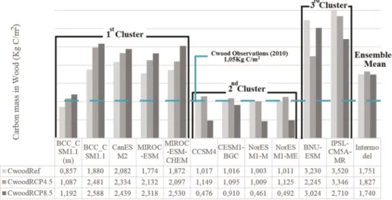
Figure 1.Thirty year average of carbon in wood stock (kg/m2) for each climate time model.

3. Results

In this section we analyze the results from carbon accumulation (in wood) and carbon sequestration throughout the Iberian Peninsula, and their comparison. We also disclose the results from the response and quantification of C feedback to changing climate variables as well as the future projections of WUE trends across the 12 CMIP5 models.

3.1. Carbon Accumulation on Wood: Forest Growth

Forest growth simulated by the CMIP5 models is illustrated in Figure 1 that shows the 30 years mean annual values of carbon mass in wood (Cwood) per square meter under the historical period (CwoodHisto) and under future scenarios (CwoodRCP4.5and CwoodRCP8.5). MPI-ESM-LR is not included since there were no available data. The dashed line refers to observed data, namely, Cwood observations by remote sensing during 2010 [Thurner et al., 2013].

Three distinct clusters based on the similarities between Cwood averages and Cwood changes between scenarios appear evident. Thefirst cluster offive models (left group on Figure 1) shows an increase of Cwood relative to historical period (1970–1999), with ranges between 1.1 and 2.5 kg C/m2_{, and between 1.2 and} 2.6 kg C/m2, for RCP4.5 and RCP8.5 scenarios, respectively. BCC_CSM1.1 (m) presents substantially lower values (nearly half of Cwood) compared to the rest of the group, being closer to the second cluster of models, in terms of amount of Cwood stored.

The second cluster of models (CCSM4, CESM1-BGC, NorESM1-M, and NorESM1-ME) simulates lower amounts of Cwood (~1.0 kg C/m2_{for historical period), and a decreasing trend down to half of the Cwood during} Figure 2.Annual means of Cwood along 30 year periods segregated by family of models. (a) First family of models, historical period; (b)first family of models, RCP4.5 scenario; (c) second family of models, historical scenario; (d) second family of models, RCP4.5 scenario; (e) third family of models, historical scenario; and (f) third family of models, RCP4.5 scenario.

historical time for RCP8.5 scenario. Under RCP4.5, those models simulate a slight increase of Cwood compared to historical period; however, this increase is not as significant as in thefirst cluster of models.

The third cluster of models (BNU-ESM and IPSL-CM5A-MR) presents mean values of Cwood significantly high for historical period (above 3 kg C/m2) and distinguishable results from the previous clusters. BNU-ESM projects lower Cwood under RCP4.5 scenario than in historical and RCP8.5 scenarios, while IPSL-CM5A-MR projects decrease Cwood values for increasing CO2levels. The Cwood observations are slightly higher than the historical estimations of Cwood, for every model belonging to the second cluster and also BCC_CSM1.1, which in principle makes sense since 2010 is 10 years away from the historical period (i.e., 1970–1999).

Mean annual values of Cwood for 30 consecutive years are shown in Figure 2, for historical period (left column) and RCP4.5 scenario (right column). Under RCP4.5 scenario, the trends across the 30 year periods are not remarkable, with just a small increase along the years perceived for the second cluster of models and for the BCC models (i.e., BCC_CSM1.1 (m) and BCC_CSM1.1) during the historical period (1970–1999). CanESM2 presents a small decreasing trend within each 30 year set, for both historical and RCP4.5 scenarios. The MIROC models show the greatest slopes and a noticeable decadal-scale variability of carbon in wood storage— potentially a result of the competition modulation between vegetation and the transition between land use types. Land use is reproduced by a data set of fractional changes of land use in each grid, computed using a 10 year time step [Watanabe et al., 2011].

3.2. Carbon Sequestration: GPP and NPP Projections by Late 21st Century

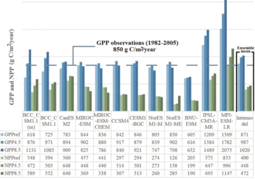
BNU-ESM estimates the lowest value of GPP for historical period (GPPHisto), around 605 g C/m2/yr, while IPSL-CM5A-MR and MPI-ESM-LR the highest records of GPPHisto, 1209 and 1509 g C/m2/yr, respectively. Under RCP4.5 scenario, estimations of GPP (GPPRCP4.5) range between 616 and 1782 g C/m2/yr (BNU-ESM and MPI-ESM-LR, respectively); while under RCP8.5, the GPP response (GPPRCP8.5) is wider, ranging between 632 and 2075 g C/m2/yr (BNU-ESM and MPI-ESM-LR, respectively) (Figure 3).

As for GPP, IPSL-CM5A-MR and MPI-ESM-LR present the highest estimated NPP values, 575 and 833 g C/m2/yr, respectively, under the RCP4.5 scenario. The lowest NPPHistoestimations are simulated by NorESM1-ME (~126 g C/m2/yr), and for future scenarios it keeps lower values compared to other models. Estimates of NPPRCP4.5range between 138 g C/m2/yr (NorESM1-ME) and 996 g C/m2/yr (MPI-ESM-LR), and of NPPRCP8.5 between 190 g C/m2_{/yr (BNU-ESM) and 1147 g C/m}2_{/yr (MPI-ESM-LR).}

Figure 3.Thirty year average of gross primary production and net primary production in the Iberian Peninsula.

From the comparison with observed data (dashed line in Figure 3), GPP during a similar historic period (1982–2005) was calculated to be 850 g C/m2/year. This value was significantly close to the averaged intermodel GPP, suggesting that the overall estimation of GPP modeled for that period is fairly plausible.

The trends of GPP and NPP projected by the ESMs for late 21st century present discrepancies among them, as shown in Figure 4, which presents the relative difference between production rates of the average pixel representing the entire IP. Most models project the averaged pixel of IP to increase GPP and NPP under RCP4.5 scenario (exceptions are for MIROC-ESM-CHEM and BNU-ESM for GPPRCP4.5,and both MIROC models, BNU-ESM and NorESM1-M for NPPRCP4.5).

The models broadly agree on GPP estimates under the RCP4.5 scenario as they all predict an increase relative to historical records, i.e., the overall estimation of relative change between RCP4.5 scenario and historical period (ΔGPPRCP4.5-Histo) is positive and the ensemble projects a 13.9% increase. The range of positive change is considerably wide, going from 1.8% (BNU-ESM) up to 41.7% (BCC_CSM1.1.(m)). For RCP8.5 scenario, ESMs present a considerable variation in magnitude and sign of GPP (ΔGPPRCP8.5-Histo), being apparent two clusters of model estimates. One composed by the BCC models, CanESM2, CESM1-BGC, BNU-ESM, IPSL-CM5A-MR, and MPI-ESM-LR which present a broad range of positive relative increase ofΔGPPRCP8.5-Histo, ranging from 4.5% (BNU-ESM) up to 83% (BCC_CSM1.1 (m)). The second group with the remaining models simulates a negative response ranging from 0.3 to 7.2% (CCSM4 and NorESM1-M, respectively).

The positive differences ofΔNPPRCP4.5-Historange between 2.6% (CESM1-BGC) and 35.7% (BCC_CSM1.1 (m)), whereas the negative changes range between 0.4% (NorESM1-M) and 2.0% (MIROC-ESM). For the RCP8.5 scenario, positive changes ofΔNPPRCP8.5-Historange between 3.5% (CCSM4) and 69.1% (BCC_CSM1.1 (m)), and negative changes between 5.3% (NorESM1-M) and 23.3% (MIROC-ESM-CHEM). NorESM1-M estimates Figure 4.The relative variation of GPP and NPP (by average pixel) between future scenarios and historical scenario.

are not included in Figure 4, since it simulates a drastic increase of NPP (around 126%) for the RCP8.5 scenario, which would make difficult its interpretation. It is noticeable that NorESM-ME presents the lowest estimate of NPPHisto(126 g C/m2/yr), which justifies the abrupt perceptual growth when compared to RCP8.5 (285 g C/m2/yr).

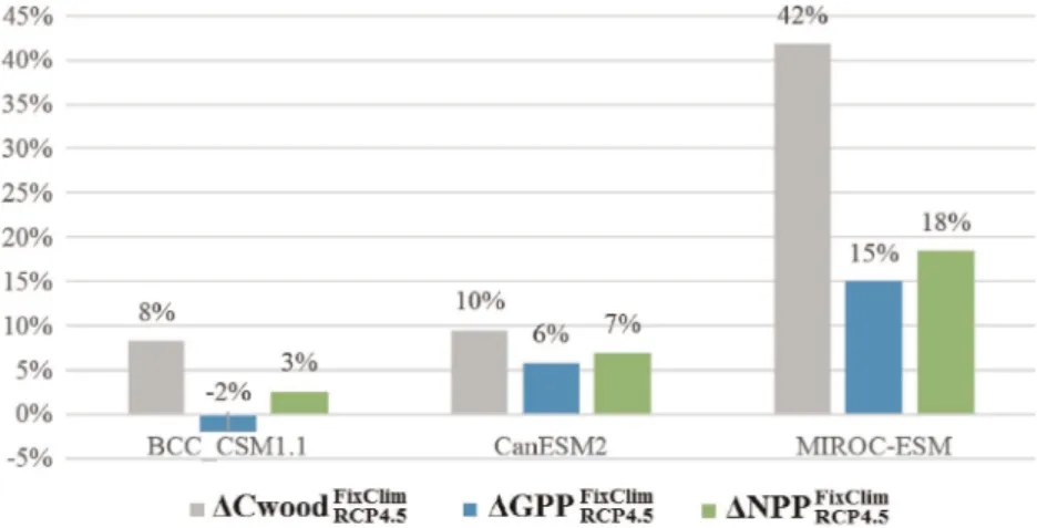
Figure 5 enables the comparison of relative changes (%) of carbonfluxes for RCP4.5 scenario, under two different conditions: (i) assuming the joint effects of climate change and increasing CO2on carbon responses and (ii) carbon cycle feedback ignores climate change induced by carbon emissions and only responds to increasing CO2. The comparison aims at understanding the isolated effect and the magnitude of CO2on carbon sequestration and accumulation in wood. We take the simulations of Cwood, GPP, and NPP from BCC_CSM1.1, CanESM2, and MIROC-CHEM models, as these are the only models providing data relative to the experiment with afixed climate and assuming the same carbon concentrations as in RCP4.5. In ascending order, GPP, NPP, and Cwood present growing positive impact of atmospheric [CO2]. MIROC-ESM simulates the highest impacts (70%) on Cwood, while vegetation production (GPP and NPP) is most impacted on simulations by CanESM2 and BCC_CSM1.1. The later tops GPP and NPP relative differences of FixClim, and RCP4.5 scenario to historical period, followed by CanESM2 and MIROC-ESM. The relative change of GPP to historical period simulated by BCC_CSM1.1 is an exception as it amounts to 34 and 31% under RCP4.5 Figure 5.Relative change (%) of Cwood, GPP, and NPP under scenario of climate change and rising CO2(RCP4.5-Histo); and

relative change of Cwood, GPP, and NPP under scenario only accounting to effect of rising CO2(FixClim-Histo).

Figure 6.Relative changes (%) of Cwood, GPP, and NPP between FixClim and RCP4.5 scenario.

scenario and FixClim scenario, respectively. Under FixClim, MIROC-CHEM changes the response sign as it simulates a positive change (16%) in NPP relative to historic period, when under climate changing conditions the response was negative ( 2%).

The estimated climate change effect on carbon cycle, relative to simulations assuming climate change and increased [CO2], can be depicted in Figure 6. The trends appear opposite from the former analysis, except for Cwood, since MIROC also projects to be greatly impacted (42%). For every model, GPP is less affected (and in the case of BCC_CSM1.1 it is negative, 2%). MIROC-ESM is the model accounting for the greatest effect of climate change on GPP and NPP, with 15 and 18%, respectively.

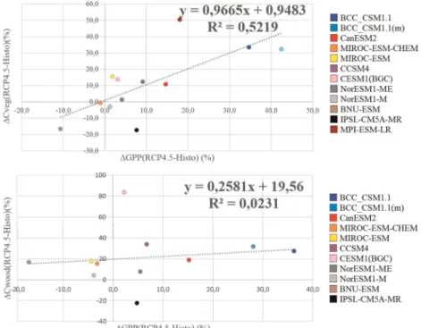
Figure 7.Relationship betweenΔGPP andΔCveg (relative variations between scenario RCP4.5 and historical period) (% versus %).

Figure 8.Relative difference (%) of temperature, precipitation, and evapotranspiration between future scenarios (RCP4.5 and RCP8.5) and historical records.

3.2.1. Comparing Carbon Sequestration With Carbon Storage

Figure 7 depicts the relationship between the relative differences (%) of GPP and carbon mass in vegetation (Cveg) between RCP4.5 scenario and historical period, as well as between NPP and carbon mass in wood (Cwood). GPP and Cveg present a linear trend line

fitting the points with anr2= 0.52, meaning that half of the total intermodel variation in projections forΔCvegRCP4.5-Histois explained by the variation presented betweenΔGPPRCP4.5-Histoprojected by the ESMs. IPSL-CM5A-MR and the MPI-ESM-LR have the greatest distance to the linear trend line and the greatest discrepancies compared to the other models. IPSL-CM5A-MR simulates an increase of 51% CvegRCP4.5-Histovariation for 18% GPPRCP4.5-Histo variation. MPI-ESM-LR presents a decrease of around

17% ofΔCvegRCP4.5-Histofor a small increase of ΔGPPRCP4.5-Histovariation (of nearly 8%). This model, along with BNU-ESM and NorESM1-M, stays below the axis referring to variation of CvegRCP4.5-Histo. For the relationship betweenΔNPPRCP4.5-Histoand ΔCwoodRCP4.5-Histo, the models present similar positions relative to axis and signs of change. The major difference lies on the slope of thefitting trend line with a slope near zero, which will have different implications when assessing causes of intermodel variations on carbonfluxes responses, explored in section 4.

3.3. Sensitivity of Carbon Fluxes to Climatic Variables

In response to the RCP scenarios, all models simulate an increase in mean annual air surface temperature. For RCP4.5 scenario, the multimodel average increases by 2.4°C (corresponding to an increase of approximately 15.9% relative to historical records) (Figure 8), with values ranging from 1.9°C (BCC_CSM1.1 (m)) to 3.6°C (MIROC models), corresponding to a relative increase of 11.9 and 22.8%, respectively. For the RCP8.5 scenario, the average increase is 4.5°C, meaning a relative difference of 28.8%. Precipitation is expected to decrease on average about 11 and 24% under scenarios RCP4.5 and RCP8.5, respectively, with broader range of values predicted by each model than in the case of air temperature. Under the RCP4.5 scenario, BCC_CSM1.1 predicts the lowest change in precipitation, around 2.4%, and MPI-ESM-LR predicts a decrease of 17.2%. Under the RCP8.5 scenario, IPSL-CM5A-MR and MIROC-ESM present the less and most marked decreases in precipitation, respectively with 19.1 and 29.0% of rainfall reduction.

Table 3 shows the sensitivity (ρ) of NPP, GPP, and Cwood to climate factors, accounting in metric terms

Ta b le 3 . Q uanti fi cat ion of Mode ls ’ Sens itiviti es of Car bon Fluxes to Tempe rature and Pre cipitation Fluxes and Atmospher ic CO 2 by Late 21st Century Under RCP4 .5 Scena rio a M odels BC C_CSM 1.1 (m) BC C_C SM1.1 BNU-ESM MIROC -ESM MIROC -ESM-CHEM C CSM4 NorESM1.1 -M No rESM1.1-ME CES M1-BGC CanESM 2 IPSL -CM5A-MR M PI-ESM -LR Pre cipitation ρ NPP P 1.54 5.30 6.19 0.06 0.14 0.37 10 .70 0.32 0.07 1.17 3.01 1.50 ρ GPP P 3.20 13.94 24.90 0.95 0.79 1.50 16 .14 1.99 0.27 2.12 7.22 2.58 ρ Cwo od P 2.66 43.78 160 .29 6.22 2.69 2.75 87 .79 2.59 0.74 3.65 16 .36 n.a. Tempe rature ρ NPP T 62.06 57 .83 4.27 0.84 1.05 9.15 0.03 5.75 4.16 22 .03 44 .13 74.89 ρ GPP T 128.60 13 0.41 23.90 17.82 15.07 40.20 17.08 34.19 19.60 37 .97 99 .80 125.46 ρ Cwo od 116.79 31 8.73 468.91 92.25 66.49 73.94 3.78 55.82 51.51 91 .68 52.51 n.a. Atm osphe ric CO 2 ρ NPP ET 0.66 0.58 0.03 0.05 0.01 0.09 0.01 0.07 0.04 0.34 0.39 0.87 ρ GPP ET 1.38 1.31 0.06 0.31 0.24 0.40 0.18 0.38 0.18 0.59 0.93 1.46 ρ Cwo od ET 1.23 3.21 5.25 1.91 1.20 0.70 0.03 0.61 0.43 1.34 0.93 n.a. a Units: Net prima ry produ ction sens itivity to precipitatio n (g C/g H2 O); NPP sens itivity to temp eratur e (g C/y r/ m 2 /°C); Gross prima ry produ ction sen sitivity to precipitat ion (g C/g H2 O ); GPP sen sitivity to temper ature (g C/y r/ m 2 /° C ); Car bon mass in wood sensitivity to precipitation (g C/g H2 O ); Cwo od sen sitivity to temper ature (g C/g H2 O ); Ne t prima ry pro duction sen sitivity to CO 2 con centrati on (g C/y r/ m 2 /ppm ); G ross pri mary produ ction sen sitivity to CO 2 concen tration (g C/y r/ m 2 /ppm) ;Carbon mas s in wood sensitivity to CO 2 conce ntration (g C/yr/ m 2 /ppm) .

the amount of annual incorporation of carbon per unit area per unit of climate variable. In regard to temperature, expressed in carbon massflux per degree Celsius (g C/yr/m2/°C), the majority of models show high production response and present a very wide range of values.ρNPPT(sensitivity of NPP to temperature) ranges from values as high as 74.9 g C/yr/m2_{/°C (MPI-ESM-LR) down to negligible values (NorESM1-M).} MIROC-ESM and NorESM1-M are the only models presenting a negative but small sign ofρNPPT, simulating the decrease of carbonflux lower than 1 g C/m2for each increasing degree Celsius.

Sensitivities to precipitation (ρNPPPandρGPPP), expressed by carbonflux per gram of water (g /yr/m2/C/g H2O), show negative responses from every model (except for MIROC-ESM). This sign is expected as it results from the quotient between positives values ofδNPP4.5-Histo(since most ESMs modeled NPP increases

relatively to historical period) and negative values ofδP4.5-Histo(as every model project rainfall decreases by 2070–2100 for RCP4.5 scenario). The less significant sensitivities are simulated by MIROC-ESM.

The GPP sensitivity to CO2is positive across all models, ranging between 0.06 and 1.46 g C/m2/ppm (BNU-ESM and MPI-ESM-LR, respectively). Most models simulate a positive response of NPP to CO2ranging between 0.04 and 0.87 g C/m2/ppm (CESM1-BGC and MPI-ESM-LR, respectively). For cases whereρNPPCO2is negative, the range was less broad, varying between 0.01 (MIROC-ESM-CHEM and NorESM1.1-M) and 0.05 g C/m2_{/ppm (MIROC-ESM).} ForρCwoodCO2most models also present positive responses (with exceptions for BNU-ESM and IPSL-CM5A-MR) (Table 4).

3.4. Water-Use Efficiency Future Projection Changes

Almost every model simulates a decrease in mean annual evapotranspiration, between 2.2% (BNU-ESM) and 14.1% (MPI-ESM-LR), under RCP4.5. BCC_CSM1.1 and the NorESM models project small positive increases for this variable, around 1.2% (BCC_CSM1.1) and 5.3 and 2.6% Table 4. Sensitivity of Carbon Variables to CO2Under RCP4.5a

Models BCC_CSM1.1 (m) BCC_CSM1.1 BNU-ESM MIROC-ESM MIROC-ESM-CHEM CCSM4

Cwood 1.23 3.21 5.25 1.91 1.20 0.70

NPP 0.66 0.58 0.03 0.05 0.01 0.09

GPP 1.38 1.31 0.06 0.31 0.24 0.40

Models NorESM1-M NorESM1-ME CESM1-BGC CanESM2 IPSL-CM5A-MR MPI-ESM-LR

Cwood 0.03 0.61 0.43 1.34 0.93 0

NPP 0.01 0.07 0.04 0.34 0.39 0.87

GPP 0.18 0.38 0.18 0.59 0.93 1.46

a_{Units: Net primary production sensitivity to CO}

2concentration (g C/yr/ m2/ppm); Gross primary production sensitivity to

CO2concentration (g C/yr/ m2/ppm); Carbon mass in wood sensitivity to CO2concentration (g C/yr/ m2/ppm).

Figure 9.Percent change in water-use efficiency under future scenario in Iberian Peninsula.

for the NorESM1-M and NorESM1-ME, respectively). Under the RCP8.5 scenario, every model predicts a decrease in evapotranspiration (except NorESM1-M which keeps it constant) (Figure 9).

WUE simulations during historical periods ranged between 0.9 and 3.0 g C/g H2O (BNU-ESM and MPI-ESM-LR, respectively) (Figure 9). The average WUE modeled for the historical period is very close to the observation data referring to a similar period (1982–2005). Again, these values reinforce the high reliability of GPP (and evapotranspiration) estimations at least during the historical period. The mean of the modelling ensemble for WUE estimates is 20.5 and 34.0% of relative increase for RCP4.5 and RCP8.5, respectively. Every model (except NorESM1-M) presents an increased WUE under both future RCP scenarios withΔWUERCP4.5-Historanging between 5% (BNU-ESM) and 56.8% (BCC_CSM1.1 (m)). The WUE values in RCP8.5 are up to twice as high as those in the historical period, ranging between 0.9% (NorESM1-ME) and 105.3% (BCC-CSM1.1 (m)) (Figure 9). Figure 10 presents relative changes of GPP and precipitation between RCP4.5 and historical records, enabling to depict the models which GPP response decreased as a probable effect of reduced rainfall, namely, MIROC-ESM-CHEM and BNU-ESM.

4. Discussion

4.1. Forest Growth Trends in Iberian Peninsula Over the 21st Century

A common feature to every model of thefirst cluster, defined by the 21st century projections of forest growth (Figure 1), is the absence of the nitrogen (N) cycle (Table 1). This could explain the increase of carbon mass in wood (Cwood) with increasing atmospheric CO2, since there is no growth constraint from N limitation [Zaehle et al., 2010]. The same applies to the third cluster (BNU-ESM and IPSL-CM5A-LR), since this cluster projects considerable high amount of Cwood, although they do not simulate Cwood increasing straightforwardly with rising CO2levels. Both models assume vegetation competition and are partly based on the same land cover (Global Land Cover Classification) [Krinner et al., 2005], which can contribute to the high Cwood simulations.

This model segmentation by clusters, points N cycle inclusion as a major differentiator among the ESMs, more specifically at the level of trends projections for RCP8.5 scenarios and Cwood amounts. Conversely, the second cluster (composed by CSM4, CESM-BGC, and the NorESM models) runs the N cycle on its experiments, which is likely the main reason for forest reduction under RCP8.5 scenario compared to historical values. Besides the inclusion of the N cycle, as described byLawrence et al. [2011], the greatest similarity shared by this cluster is the common land model component (CLM4), with no simulation of dynamic vegetation (DV). The absence of plant community dynamics (e.g. competition, diversity) could also be behind the reasons determining forest decrease under RCP8.5 scenario, as it determines less adaptability by the vegetation.

Thefirst and second model clusters (amounting to 10 of the 12 models) are in agreement in terms of forest growth projections for scenario RCP4.5 that could potentially result from the higher CO2concentration prescribed (relative to historic period). However, it is challenging to quantify the overall effects controlling Figure 10.Assessment of hydric stress existence for RCP4.5 projected by each model.

tree growth as it is controlled by complex interactions between numerous factors such as related and nonrelated climate change factors (e.g., forest management [Lavalle et al., 2009]). In fact, one relevant feature to take into account during forest growth projections is the land use and land cover use change (LULCC), with consequences both at the carbon cycle level and vegetation cover. For example, it changes the allocation of the carbon reservoirs among the PFT, which could result in extra CO2emissions as a consequence of transitional changes in carbon pools. Nevertheless, as concluded from Figure 2, LULCC is not relevant, at least for a year-based level for the covered periods. By intercomparing each 30 year period, there is no correspondence between LULCC and the Cwood behavior from year to year. IPSL-CM5A-MR and the second model cluster translate a clear evidence of this. Both are following the same harmonization protocol [Hurtt et al., 2011] (Table 1), but that is not reflected within a 30 year sequential behavior in regard to Cwood accumulation (Figure 2).

As for the underlying processes dominating carbon storage in wood, we would suggest that models falling in the same cluster likely make similar assumptions about the mechanisms regulating carbon incorporation on wood. BNU-ESM and IPSL-CM5A-MR can be considered exceptions as their trends vary between themselves and strongly vary from the twofirst clusters. As such, these models present a clear structural difference compared to the others, and we hypothesize that ecophysiology differences are the main reason.

4.2. CO2Fertilization Effect in Iberian Peninsula by Late 21st Century

The interannual variability shown for annual GPP and NPP does not promptly link each model to one of the three clusters earlier defined. Based on sign and magnitude of vegetation response to climate change and prescribed [CO2], two major clusters are observed (Figure 4). Thefirst cluster, including seven models (BCC models, MPI-ESM-LR, CanESM2, IPSL-CM5A-MR, CCSM4, and CESM1-BGC), predicts increases of net and gross production, under both RCP4.5 and RCP8.5 scenarios (with exception for CCSM4 under RCP8.5). These results imply that these models assume the vegetation of the IP to be a stronger sink of CO2by late century.

The second cluster, comprising the remaining models, simulates decreases of GPP and NPP, or slight increases for GPP under RCP4.5 (as is the case of the NorESM models and MIROC-ESM), suggesting that some models may be projecting the IP as a source of CO2. The MIROC models show the most distinct trends, simulating significant decreases of NPP under RCP8.5. Although not so marked, GPP also decreases under RCP8.5. BNU-ESM and NorESM1-M models also simulate future decrease of NPP, although not so strong. The inclusion of N cycle and dynamic vegetation seemingly has little perceivable effect on assigning models to the clusters (Table 1).

Figure 4 reinforces the suggestion that positive variations of NPP and GPP from historical to future scenarios are linked to the CO2fertilization effect in most cases. The experiment FixClim enabled to disclose the sole effect of CO2, i.e., carbon cycle feedback is only forced by changes in CO2concentrations and changes in climate changes derived by that are ignored (Figure 5). The increase of positive response discloses the strength of rising CO2concentration alone on the carbon cycle as simulated by these models. BCC_CSM1.1 and CanESM2 present a stronger primary production feedback to CO2than MIROC-ESM. The enhanced terrestrial photosynthesis due to CO2enriching projected by the two prior models (Figure 4) agrees with thosefindings and with consequent increased WUE values (Figure 9).

The positive results in Figure 6, translating the susceptibility of vegetation only to climate change triggered by CO2atmospheric concentrations, show that the variables more affected by climate change are Cwood, NPP, and GPP, in decreasing order. This suggests that models simulate climate change to play a greater role on carbon allocation rather than carbon (net and gross) sequestration. The MIROC-ESM shows most contrasting responses to climate change, meaning that it is more controlled by climate change than effects of increasing CO2,which consolidate the last conclusion. Thesefindings are in agreement with previous exercises [Arora et al., 2013], where MIROC had the strongest land carbon-climate feedback among several ESMs (BCC_CSM1.1 and CanESM2 were also part of the study). The highest impact of climate change variables on MIROC and lowest CO2-driven response could explain the fact that it is one of the few models that may be projecting the Iberian Peninsula as a carbon source (Figure 4) along with the fact that it is projecting the strongest decreases in precipitation (Figure 8).

constraints to N cycle raises the strong possibility that these two models might be potentially overestimating the 21st century response of carbon sequestration and storage. Moreover, the BCC models do not simulate dynamic vegetation, and thus, the composition and abundance of plant functional types (PFTs) within a grid cell are time invariant [Wu et al., 2013]. This means that BCC models neglect the changes in physical and biogeochemical properties of the vegetation, following actual land cover changes. Our assessment is corroborated byBrovkin et al. [2013], who highlight the importance of LULCC on carbonfluxes projections and the risks of overlooking or underestimating NPP. Land use change is a critical component of the terrestrial carbon cycle and it is likely the driver of some of the intermodel variations in carbonfluxes results.

Besides looking into differences in model structure and parameterizations, the causes of model discrepancies can be assessed through the relationships between variables (Figure 7). The slope (close to 1) of the trend line

fitted to the relationship between the variation of GPP and variation of carbon mass in vegetation (Cveg), suggests that the discrepancies between models rely on modeling ecophysiology. That slope implies a strong linear relationship betweenΔCveg andΔGPP across models, meaning that the effect of changes in vegetation cover, for instance, do not affect this relationship. On the other hand, the slope of the trend linefitting the relationship betweenΔNPP andΔCwood is significantly lower than 1. From these results, we hypothesized that, when taking into account the net uptake of carbon and its incorporation in wood pool, the different responses between ESMs are mostly due to parameterization discrepancies. It should be noticed that biogeochemical processes underlying the gross uptake of carbon into vegetation as a whole are better known than allocation of net carbonflux to a specific pool (wood). In fact, the outputs for Cwood seem to be highly land cover dependent as noticed before.

4.2.1. Rainfall Reduction and Water-Use Efficiency Trends

Almost every model simulates increasing WUE with increasing [CO2] levels (Figure 9), which implies an increased carbon sequestration despite the nearly 16% of rainfall reduction projected by the ESMs ensemble (Figure 8). These results are consistent with a significant CO2fertilization effect. Therefore, the rise of CO2is overcompensating for growth declines, anticipated from a drier climate, suggesting a stronger effect of CO2 fertilization than water reduction, likely detectable in other forests across the Mediterranean [Koutavas, 2013]. Nevertheless, this assertion is questionable as the IP is broadly characterized as a water-limited region [Reichstein et al., 2002]. On one hand, it is widely accepted that increased WUE composes an expectable response to a drier climate due to reduced stomatal conductance [Prior et al., 2011]. Furthermore, that mechanism regulating stomatal behavior is broadly adopted in ecosystem models. But, on the other hand, some studies found that WUE is also impacted by severe droughts [Lu and Zhuang, 2010]. We also hypothesize that CO2fertilization effect might be overrated leading to the overestimation of carbonfluxes, which in part is supported byZhou and Riley[2012]. Models belonging to thefirst cluster corroborate this assumption since they present a doubled increase of WUE between RCP4.5 and RCP8.5 (Figure 9). NorESM1-M model should be referred as exception, as it projects decreased WUE for future scenarios.

With rainfall reduction (Figure 8), BNU-ESM and MIROC-ESM-CHEM are the only models simulating decreases of GPP (Figures 4 and 10), showing to undergo hydric stress under the RCP4.5 scenario. Despite the high consistency on WUE increase and lack of hydric stress, the results of models are highly uncertain.Orlowsky and Seneviratne[2013] emphasize the large uncertainty in the quantification and projection of drought on the regional scale, and even so their studies suggested that droughts have increased in the Mediterranean and are projected to increase further. Regional drought hot spot hardly displays any trend over the last decades. However, soil moisture anomalies from CMIP5 are suggesting increasing soil moisture in the Mediterranean [Orlowsky and Seneviratne, 2013], which is likely in agreement with our results since evapotranspiration is decreasing across models (Figure 8). However, the uncertainty in the representation of soil moisture-climate feedbacks in current models [e.g.,Koster et al., 2004] and the overall spread of climate models with respect to drought projections [Seneviratne et al., 2013] emphasize the need for a deeper evaluation of the underlying factors on the hydrological cycle and land water balance.

RCP4.5. The trends of evapotranspiration rates could also suggest that it is contributing to soil moisture which in turn will benefit continued carbon sequestration despite decreasing precipitation rates.

4.3. Drivers of Carbon Cycle Feedbacks and Quantified Sensitivities

The relative changes in climate and evapotranspiration data show similar trends across models, although with few exceptions (Figure 8), which could relate to changes in carbonflux projections. For temperature, every model predicts increasing temperature with CO2rise by 2070–2099. The MIROC model simulates the most marked temperature increases (which agrees withfindings inBrovkin et al. [2013]), translating the most marked reductions of precipitation, specially accentuated for RCP8.5. MIROC’s strong climate-change-driven responses (most markedly for RCP8.5) may be turning the IP forests into a source of CO2(Figure 4). On the other hand, MPI-ESM-LR projects similar decrease in precipitation (although not so strong temperature increase) and is the third model with higher and positive GPP and NPP responses. Furthermore, when comparing modelling aspects, both MIROC and MPI-ESM-LR do not present strong differences, as they have dynamic vegetation, LULCC, and absence of N cycle. The most evident differences between these two models are the simulated temperatures, which could raise the question that MIROC is assuming temperature to be a constraint to production (by reaching an optimal peak, for instance). Hence, the modelling of ecophysiology would explain the difference. Moreover, the discrepancy in the approach used for carbonflux calculations and in the different representations of the underlying chemical and physical processes can also explain the differences.

The analysis of quantified sensitivities is of great interest as it enables to disclose the importance of model input imprecisions on modeling processes. However, intermodel comparisons of sensitivities should be approached with caution. They should only be undertaken toward a specific variable at a time or variables sharing the same units (e.g., NNP and GPP). Hence, the quantification of sensitivities should not be cross-checked straightforwardly in order to prevent false assumptions—as the differences of magnitudes rely on the units adopted for each variable. Also, it should be noted that sensitivities were calculated solely for RCP4.5 scenario.

The models belonging to the cluster defined by high production rates (BCC models, CanESM2, IPSL-CM5A, and MPI-ESM-LR) (Figure 4) naturally demonstrate a high and positive sensitivity toward temperature (Table 3). The remaining models also show a positive response of GPP to this variable. However, for NPP, two models disagree with the sign of the response, as they simulate small carbon loss per increased degree Celsius (e.g., 0.84 g C/yr/m2/°C for MIROC-ESM). Again, the fact that the modelling ensemble presents rather more agreement on GPP sensitivities rather than NPP could be due to the processes determining either the accumulation of carbon in vegetation or losses through respiration. This hypothesis is also in accordance with thefindings from Figure 7, as there is a stronger intermodel correlation between variations of GPP and Cveg than between variations of NPP and Cwood (since more and complex processes are related). As for the quantifications of sensitivity to CO2, the multimodel positive GPP response to increasing CO2 concentrations could again suggest that the carbon sequestration is improved owing to CO2fertilization effect as photosynthesis process is enhanced.

Regarding now specifically the sensitivities of Iberian Peninsula forests, every model simulates Cwood increase per unit of temperature. Exceptions are natural for BNU-ESM and IPSL-CM5A, which present a strongly marked negative sensitivity under RCP4.5 (Figure 1), potentially related to considerable differences between the parameterization of these models, as discussed before.

It should also be borne in mind that this sensitivity analysis would be composed of a more meaningful and reliable result if the carbon-related variables (i.e. NPP, GPP and Cwood) were compared with climate variables (i.e., precipitation and temperature), resulting from the running experiment where carbon cycle is ignoring the effects of CO2. The same note applies to sensitivities toward CO2. Interesting results would appear if the carbonfluxes from runs where vegetation is ignoring climate change and only accounting for CO2increase (which is the case of the FixClim experiment) would be available for all models. However, as stated before, for this case, only three models had such data available.

4.4. Sources of Uncertainties and Improvements to CMIP5 Models

cycle-climate feedback is necessary for lessening uncertainty between Earth System Models [Friedlingstein et al., 2006], contributing to their improvement.

It should be noted that the experiments assessed were performed with prescribed CO2atmospheric concentrations, and a full assessment of biogeochemical effects of RCP scenarios and driving variables on carbon sequestration in IP forests is not regarded in this study. Notwithstanding, our results point out some features as indicators of uncertainties or limits to models—both related to model structure or to climate drivers. There are a broad number of factors that may contribute to data divergence: (i) uncertainties in the data, (ii) incorrect representation of environmental drivers in the models, and (iii) incorrect or discrepancies in model ecophysiology, structure, or parameterization of the response to driving variables.

Differences in Cwood must be due to different model skills in simulating GPP as well as carbon allocation or in representing the response of Cwood to drivers through model parameterization and structure. BNU-ESM and IPSL-CM5AMR, for instance, show a unique disconnection between NPP and wood carbon, which could be due to differences in the way plant biomass is allocated to wood pool in the model. A further investigation in these particular modelling structures should be able to provide a definitive explanation. Our results also show the importance of parameterization, land model component, and inclusion of N in predictions of carbon wood incorporation, as they were key features to assign models in distinct clusters. Dynamic vegetation is another source of uncertainty, since it changes allocation with climate change variables.

The results show that differences in NPP did not contribute significantly to differences in Cwood across ESMs. Nevertheless, as NPP is a significant driver of Cwood, this lack of connection between these two responses, suggest them as focal variables for improving forest carbon estimates. Given the large range of NPP across ESMs, it is a possibility that revising photosynthesis and respiration algorithms in some ESMs could lead to more consistent NPP results. However, even with the improvement of temperature, precipitation, and evapotranspiration, these drivers are always constrained to limitations in the ability to explain NPP trends in the IP with the current model structures, as similar drivers (Figure 8) lead to unrelated intermodel responses (Figure 4). The lack of a meaningful response to precipitation, i.e., barely perceivable correspondence between ΔNPP andΔPrecipitation, though actual soil moisture and available water to the plants could be addressed here, could be in fact another dominant source of uncertainty. Additionally, we saw no pattern in changing climate variables that would fall in two distinct clusters, as simulations of productions do. Also, the structural features examined did not clearly relate to differences in the model projections, with respect to the assumption of N cycle, or temperature and moisture sensitivity functions (Table 1).

In fact the loss of pattern or agreement of ESMs under higher CO2forcing (RCP8.5), in respect to the potential shift of the IP forests into a source of CO2, can be an indicator of uncertainty due to differences in model parameterization. It should be reinforced that the experiments assessed were performed always for the same time span from historical period (1970–1999) and with prescribed CO2forcing, and a full assessment of biogeochemical effects of RCP scenarios on carbon sequestration (and storage in wood pools) is beyond the scope of this study.

These are also key processes with no margin of doubt which request for more understanding and improvement since they play extremely important roles in the terrestrial carbon cycle—more specifically on carbon sequestration. These key processes include the strength of CO2fertilization (to which there are no data available for all models) and the removal or lessening of climate change uncertainty. These processes gather a great uncertainty as they compete, posing challenges in assessing their main roles on carbon cycle feedback. This is in part resulting from the lack of understanding that the drivers present in the biosphere component. Also, given the large range of evapotranspiration and GPP across ESMs, it may be possible to improve WUE simulations by reviewing photosynthesis and stomatal conductance algorithms in some of the ESM, so that WUE would become more consistent among the models.

Moreover, despite the almost unanimous optimistic results (for RCP4.5) (for forest growth and carbon sequestration), it should be borne in mind that elevated CO2also changes plant morphology and the spatial patterns of plant species. These results should also be handled cautiously since Mediterranean terrestrial ecosystems are mostly constrained by droughts which, along with increasedfire risk and insect pathogen damage [Lindner et al., 2010], make it difficult to predict how the NPP or GPP will change in the long term at whole ecosystem level.

Nevertheless, despite the varied magnitudes and signs of model outputs, they enabled to draw several conclusions out of model responses regarding possible main drivers of carbon sequestration and wood accumulation, thus determining model differentiators. Improvements to these features, such as stronger confidence on the roles of CO2fertilization effect and the incorporation of N cycle as well as land cover change are major features for predicting future trends of forest growth and carbon sequestration with more confidence.

5. Conclusions

This paper proposed a three-component framework to analyze long-term results from 12 models from the CMIP5 on (1) primary productivity and forest growth; (2) carbon sequestration and quantification of its sensitivity to climate variables, and (3) water-use efficiency under prescribed atmospheric CO2concentration scenarios in the Iberian Peninsula. The results support the following statements:

1. The majority of the models’projections simulate forest growth by 2070–2099 relative to historic values (1970–1999) under RCP4.5 scenario. Under the RCP8.5 scenario the results have a broader variation both in magnitude and sign. The main sources of divergences in carbon mass in wood (Cwood) predictions, could be attributed to model structures, such as N cycle absence/presence, land model component, land cover data, and parameterization resulting in three distinct clusters of ESMs.

2. Increases in GPP are consistent across ESMs under RCP4.5 scenario (1.8%–41.7%). When forced by RCP8.5 atmospheric CO2concentration, models simulate large spread responses and results are less conclusive, as seven models projecting both GPP and NPP to increase (up to 83% and 69%, respectively), while the remaining models may project the IP as a carbon source by late century. ESMs divergences in carbon feedbacks are likely being highly impacted by parameterization divergences and susceptibility to either climate change or CO2fertilization effect, which raised hypothesis of overestimations.

3. Results suggest that rising CO2has the potential to partially alleviate the adverse effects of drought on primary production, as water-use efficiency is projected to increase by all ESMs, having a model ensemble mean around 21% and 34%, under RCP4.5 and RCP8.5 scenarios, respectively. Given the considerable wide intermodel variation and projected rainfall reductions ( 11% and 24%), these results emphasize the need to improve our understanding of water stress, soil moisture, and current quantification of CO2 fertilization effect.

Overcoming gaps in knowledge is of top importance to strengthen confidence in ESMs. This paper addresses proposals to improve the ability to predict the response of the carbon cycle to climate change in drought prone ecosystems. More reliable predictions are important assets to provide valid information to policy makers about the potential impacts of carbon emissions and likely outcomes for forest and forestry-related services.

References

Ahlström, A., G Schurgers, A Arneth, and B Smith (2012), Robustness and uncertainty in terrestrial ecosystem carbon response to CMIP5 climate change projections,Environ. Res. Lett.,7(4), 044008, doi:10.1088/1748-9326/7/4/044008.

Anav, A., G. Murray-Tortarolo, P. Friedlingstein, S. Sitch, S. Piao, and Z. Zhu (2013), Evaluation of land surface models in reproducing satellite derived Leaf Area Index over the high-latitude Northern Hemisphere. Part II: Earth system models,Remote Sens.,5, 3637–3661, doi:10.3390/rs5083637.

Arora, V. K., and G. J. Boer (2010), Uncertainties in the 20th century carbon budget associated with land use change,Global Change Biol., 16(12), 3327–3348, doi:10.1111/j.1365-2486.2010.02202.x.

Arora, V. K., et al. (2013), Carbon–concentration and carbon–climate feedbacks in CMIP5 earth system models,J. Clim.,26, 5289–5314, doi:10.1175/JCLI-D-12-00494.1.

Benoit, G., and A. Comeau (Dir.) (2005),Méditerranée, Les Perspectives du Plan Bleu sur l’Environnement et le Développement, Ed. de l’Aube et Plan Bleu, p. 428, Routledge, Earthscan, London.

Bertini, G., T. Amoriello, G. Fabbio, and M. Piovosi (2011), Forest growth and climate change: Evidences from the ICP-Forests intensive monitoring in Italy,iForest,4, 262–267, doi:10.3832/ifor0596-004.

Acknowledgments

The research presented in the paper was partially funded by Fundação Ciência e Tecnologia in Portugal through project UID/AMB/04085/2013. The data for this paper are available at Earth System Grid Federation (ESGF) gateways of the Program for Climate Model Diagnosis and Intercomparison (PCMDI) (http://pcmdi9. llnl.gov/esgf-web-fe/), and the Norwegian Storage Infrastructure project (NorStore) (http://noresg.norstore.no/esgf-web-fe/). The authors wish to thank the follow-ing for their contribution to this study: Xueli Shi and Li Zhang for advice on BCC_CSM1.1 and BCC-CSM1-1-M mod-els, Duoying Ji for advices on BNU-ESM and some enlightenments regarding its data, Chao Yue for advice on ORCHIDEE, Ingo Bethke and Jerry Tjiputra for their help and clarification on CO2data sets for the NorESM1-M

and NorESM1-ME models, Shingo Watanabe and Michio Kawamiya for their advices on models MIROC-ESM and MIROC-ESM-CHEM, Gary Strand for clarifications regarding CESM1-BGC and CCSMA model, Vivek Aurora for clarifications on CanESM2 model, Karl Taylor for the information provided regarding CMIP5 data experiments, Pedro Rebelo for his helpful readings, and Martin Thurner for kindly provid-ing Cwood data from remote sensprovid-ing observations and Ulrich Weber for kindly providing the GPP observation-based datasets.

Boé, J., and L. Terray (2008), A weather-type approach to analyzing winter precipitation in France: Twentieth-century trends and the role of anthropogenic forcing,J. Clim.,21, 3118–3133, doi:10.1175/2007JCLI1796.1.

Brovkin, V., et al. (2013), Effect of anthropogenic land-use and land-cover changes on climate and land carbon storage in CMIP5 projections for the twenty-first century,J. Clim.,26, 6859–6881, doi:10.1175/JCLI-D-12-00623.1.

Ciscar, J. C., et al. (2011), Physical and economic consequences of climate change in Europe,Proc. Natl. Acad. Sci. U.S.A.,108, 2678–2683, doi:10.1073/pnas.1011612108.

Dufresne J. L., et al. (2013), Climate change projections using the IPSL-CM5 Earth System Model: From CMIP3 to CMIP5,Clim. Dyn., 40(9–10), 2123–2165, doi:10.1007/s00382-012-1636-1.

Frank, D., M. Reichstein, F. Miglietta, and J. S. Pereira (2013), Impact of climate variability and extremes on the carbon cycle of the Mediterranean region, inRegional Assessment of Climate Change in the Mediterranean, Volume 2,Advances in Global Change Research, vol. 51, edited by A. Navarra, and L. Tubiana, pp. 31–47, Springer, Dordrecht, Netherlands, doi:10.1007/978-94-007-5772-1_3. Friedlingstein, P., et al. (2006), Climate–carbon cycle feedback analysis: Results from the C4MIP model intercomparison,J. Clim.,19,

3337–3353, doi:10.1175/JCLI3800.1.

García-Herrera, R., D. Paredes, R. M. Trigo, I. F. Trigo, E. Hernández, D. Barriopedro, and M. A. Mendes (2007), The outstanding 2004/05 drought in the Iberian Peninsula: Associated atmospheric circulation,J. Hydrometeorol.,8(3), 483–498, doi:10.1175/JHM578.1.

Gaucherel, C., J. Guiot, and L. Misson (2008), Changes of the potential distribution area of French Mediterranean forests under global warming,Biogeosciences,5, 1493–1504.

GCESS (2012), BNU-ESM. [Available at http://esg.bnu.edu.cn/BNU_ESM_webs/htmls/index.html, Accessed on 17th November 2014.] Giorgetta, M. A., et al. (2013), Climate and carbon cycle changes from 1850 to 2100 in MPI-ESM simulations for the Coupled Model

Intercomparison Project phase 5,J. Adv. Model. Earth Syst.,5(3), 572–597, doi:10.1002/jame.20038. Giorgi, F. (2006), Climate change hot-spots,Geophys. Res. Lett.,33, L08707, doi:10.1029/2006GL025734.

Giorgi, F., and P. Lionello (2008), Climate change projections for the Mediterranean region,Global Planet. Change,63, 90–104, doi:10.1016/ j.gloplacha.2007.09.005.

Hurtt, G. C., S. Frolking, M. G. Fearon, B. Moore, E. Shevliakovas, S. Malyshev, S. W. Pacalas, and R. A. Houghton (2006), The underpinnings of land-use history: Three centuries of global gridded land-use transitions, wood-harvest activity, and resulting secondary lands,Global

Change Biol.,12, 1208–1229, doi:10.1111/j.1365-2486.2006.01150.x.

Hurtt, G. C., et al. (2009), Harmonisation of global land-use scenarios for the period 1500–2100 for IPCC-AR5,iLEAPS Newsl.,7, 6–8. Hurtt, G. C., et al. (2011), Harmonization of land-use scenarios for the period 1500–2100: 600 years of global gridded annual land-use

transitions, wood harvest, and resulting secondary lands,Clim. Change,109, 117–161, doi:10.1007/s10584-011-0153-2. Ji, D., et al. (2014), Description and basic evaluation of BNU-ESM version 1,Geosci. Model Dev. Discuss.,7, 1601–1647, doi:10.5194/

gmdd-7-1601-2014.

Justice, C. O., J. R. G. Townshend, E. F. Vermote, E. Masuoka, R. E. Wolfe, N. Saleous, D. P. Roy, and J. T. Morisette (2002), An overview of MODIS land data processing and product status,Remote Sens. Environ.,83, 3–15, doi:10.1016/S0034-4257(02)00084-6.

Keenan, T., J. M. Serra, F. Lloret, M. Ninyerola, and S. Sabate (2011), Predicting the future of forests in the Mediterranean under climate change, with niche- and process-based models: CO2matters!,Global Change Biol.,17, 565–579.

Kelemen, A., W. Munch, H. Poelman, Z. Gakova, L. Dijkstra, and B. Torighelli (2009), The climate change challenge for European regions, Background Document to Commission Staff Working Document Sec (2008) 2868 Final, Regions 2020, An Assessment of Future Challenge for EU Regions. Koster, R. D., et al. (2004), Regions of strong coupling between soil moisture and precipitation,Science,305, 1138–1140.

Kottek, M., J. Grieser, C. Beck, B. Rudolf, and F. Rube (2006), World map of the Köppen-Geiger climate classification updated,Meteorol. Z., 15(3), 259–263, doi:10.1127/0941-2948/2006/0130.

Koutavas, A. (2013), CO2fertilization and enhanced drought resistance in Greekfirs from Cephalonia Island, Greece,Global Change Biol., 19(2), 529–539, doi:10.1111/gcb.12053.

Krinner, G., N. Viovy, N. de Noblet-Ducoudré, J. Ogeé, J. Polcher, P. Friedlingstein, P. Ciais, S. Stitch, and I. C. Prentice (2005), A dynamic global vegetation model for studies of the coupled atmosphere-biosphere system,Global Biogeochem. Cycles,19, GB1015, doi:10.1029/2003GB002199. Lavalle, C., F. Micale, T. D. Houston, A. Camia, R. Hiederer, C. Lazar, C. Conte, G. Amatulli, and G. Genovese (2009), Climate change in Europe. 3.

Impact on agriculture and forestry. A review,Agron. Sustainable Dev.,29(3), 433–446.

Lawrence, D., et al. (2011), Parameterization improvements and functional structural advances in version 4 of the Community Land Model,

J. Adv. Model. Earth Syst.,3, M03001, doi:10.1029/2011MS000045.

Lawrence, P. J., and T. N. Chase (2007), Representing a new MODIS consistent land surface in the Community Land Model (CLM 3.0),

J. Geophys. Res.,112, G01023, doi:10.1029/2006JG000168.

Lindner, M., et al. (2010), Climate change impacts, adaptive capacity, and vulnerability of European forest ecosystems,For. Ecol. Manage., 259(4), 698–709.

Lu, X., and Q. Zhuang (2010), Evaluating evapotranspiration and water-use efficiency of terrestrial ecosystems in the conterminous United States using MODIS and AmeriFlux data,Remote Sens. Environ.,114, 1924–1939, doi:10.1016/j.rse.2010.04.001.

Montaldo, N., J. D. Albertson, and M. Mancini (2008), Vegetation dynamics and soil water balance in a water-limited Mediterranean ecosystem on Sardinia, Italy,Hydrol. Earth Syst. Sci. Discuss.,5, 219–255, doi:10.5194/hess-12-1257-2008.

Moss, R. H., et al. (2010), The next generation of scenarios for climate change research and assessment,Nature,463(7282), 747–756, doi:10.1038/nature08823.

Norby, R. J., et al. (2005), Forest response to elevated CO2is conserved across a broad range of productivity,Proc. Natl. Acad. Sci. U.S.A., 102(50), 18,052–18,056, doi:10.1073/pnas.0509478102.

Oleson, K. W., et al. (2010), Technical description of version 4.0 of the Community Land Model (CLM),NCAR Technical Note NCAR/TN-478 +STR, National Center for Atmospheric Research.

Orlowsky, B., and S. I. Seneviratne (2013), Elusive drought: Uncertainty in observed trends and short- and long-term CMIP5 projections,

Hydrol. Earth Syst. Sci.,17, 1765–1781, doi:10.5194/hess-17-1765-2013.

Prior, S. A., G. B. Runion, C. Marble, H. Rogers Jr., C. Gilliam, and H. Torbert (2011), A review of elevated atmospheric CO2effects on plant growth and water relations: Implications for horticulture,HortScience,46(2), 158–162.

Quézel, P. (1985), Definition of the Mediterranean region and the origin of itsflora, inPlant Conservation in the Mediterranean Area, Geobotany, vol. 7, edited by C. Gomez-Campo, pp. 9–24, Dr. W. Junk, Dordrecht, Netherlands.

Reichstein, M., J. D. Tenhunen, O. Roupsard, J. M. Ourcival, S. Rambal, S. Dore, and R. Valentini (2002), Ecosystem respiration in two Mediterranean evergreen Holm Oak forests: Drought effects and decomposition dynamics,Funct. Ecol.,16, 27–39.

Seneviratne, S. I., et al. (2013), Impact of soil moisture-climate feedbacks on CMIP5 projections: First results from the GLACE-CMIP5 experiment,Geophys. Res. Lett.,40, 5212–5217, doi:10.1002/grl.50956.

Seufert, G., D. Kotzias, C. Sparta, and B. Versino (1995), Volatile organics in Mediterranean shrubs and their potential role in a changing environment, inAnticipated Effects of a Changing Global Environment on Mediterranean Type Ecosystems, edited by W. C. Oechel and J. M. Moreno, pp. 343–370, Springer, New York.

Sitch, S., et al. (2008), Evaluation of the terrestrial carbon cycle, future plant geography and climate-carbon cycle feedbacks usingfive Dynamic Global Vegetation Models (DGVMs),Global Change Biol.,14, 1–25, doi:10.1111/j.1365-2486.2008.01626.x.

Taylor, K. E., R. J. Stouffer, and G. A. Meehl (2012), An overview of CMIP5 and the experiments design,Bull. Am. Meteorol. Soc.,93(4), 485–498, doi:10.1175/BAMS-D-11-00094.1.

Thurner, M., et al. (2013), Carbon stock and density of northern boreal and temperate forests,Global Ecol. Biogeogr.,23, 297–310, doi:10.1111/ geb.12125.

Tjiputra, J. F., M. Bentsen, C. Roelandt, J. Schwinger, and C. Heinze (2013), Evaluation of the carbon cycle components in the Norwegian Earth System Model (NorESM),Geosci. Model Dev.,6, 301–325, doi:10.5194/gmd-6-301-2013.

Tubiello, F. N., J. F. Soussana, and S. M. Howden (2007), Crop and pasture response to climate change,Proc. Natl. Acad. Sci. U.S.A.,104(50), 19,686–19,690.

Watanabe, S., et al. (2011), MIROC-ESM 2010: Model description and basic results of CMIP5-20c3m experiments,Geosci. Model Dev. Discuss.,4, 1063–1128, doi:10.5194/gmdd-4-1063-2011.

Wu, T., et al. (2013), Global carbon budgets simulated by the Beijing Climate Centre Climate System Model for the last century,J. Geophys.

Res. Atmos.,118, 4326–4347, doi:10.1002/jgrd.50320.

Zaehle, S., A. D. Friend, P. Friedlingstein, F. Dentener, P. Peylin, and M. Schulz (2010), Carbon and nitrogen cycle dynamics in the O-CN land surface model: 2. The role of the nitrogen cycle in the historical terrestrial C balance,Global Biogeochem. Cycles,24, GB1006, doi:10.1029/ 2009GB003522.

Zhou, J., and W. J. Riley (2012), Quantifying the response of terrestrial carbonfluxes to future climate change: Results from CMIP5 Earth System Models simulations, Abstract B13B-0515 presented at Fall Meeting 2012, AGU, San Francisco, Calif.