www.adv-radio-sci.net/5/385/2007/ © Author(s) 2007. This work is licensed under a Creative Commons License.
Radio Science
Numerical modeling of the equatorial electrojet UT-variation on the
basis of the model GSM TIP
M. V. Klimenko1, V. V. Klimenko2, and V. V. Bryukhanov1 1Kaliningrad State Technical University, Kaliningrad, Russia 2West Department of IZMIRAN, Kaliningrad, Russia
Abstract. In the presented work the results of numerical modeling of the UT-variation of the equatorial electrojet, ex-ecuted on the basis of the model GSM TIP are presented, taking into account the dynamo electric fields generated by thermospheric winds in a current-carrying layer of the iono-sphere at heights 80–175 km above a surface of the Earth. To the Global Self-consistent Model of the Thermosphere, Ionosphere and Protonosphere (GSM TIP), developed in WD IZMIRAN, a new block for the calculation of electric fields in the ionosphere has been added. In this block the solu-tion of the three-dimensional equasolu-tion describing the con-servation law of the full current in the Earth’s ionosphere is reduced to the solution of the two-dimensional equation by integration along geomagnetic field lines. Calculations of pa-rameters of the near-Earth space plasmas have been executed for quiet equinoctial conditions on 22 March 1987 during the minimum of solar activity.
It has been shown, that there is a distinct semidiurnal har-monic in the diurnal behavior of the linear density of the equatorial electrojet with maxima at 23:00 UT and 15:00 UT, as well as with minima at 06:00 UT and 20:00 UT. The great-est and smallgreat-est values of the peak intensity of the equatorial electrojet with respect to the diurnal behavior can differ by a factor of two. The longitudinal extent of the area of the equatorial electrojet does hardly show any UT-variation, but the greatest longitudinal extent is at 06 UT. With the growth of the peak intensity of the equatorial electrojet its latitudi-nal extent also increases (on∼5–10◦) a little. At the same
time the equatorial electrojet in the maxima of intensity has approximately an identical width, whereas in the minima the electrojet is narrow in the morning and wide in the afternoon. As for the surface density of the equatorial electrojet, its UT-variation is much weaker and equals ∼1–3 A/km2 and the peak intensity is equal∼15–20 A/km2. The latitudinal extent of the surface density of the equatorial electrojet is maximal at 23:00 UT and 15:00 UT and minimal at 06:00 UT and 20:00 UT.
Correspondence to:M. V. Klimenko (maksim.klimenko@mail.ru)
1 Introduction
The equatorial ionosphere is unique in many respects. Global scale dynamo action, i.e. the generation of currents by elec-tromotive forces due to tidal winds results in the generation of planetary scale east-west electric fields at low latitudes around the geomagnetic equator. These electric fields, in combination with the north-south magnetic fields, cause dif-ferent geophysical phenomena near the geomagnetic equator. The most important equatorial ionospheric phenomena are: the equatorial ionization anomaly (or Appleton anomaly), the equatorial electrojet, and the generation of plasma density irregularities. An outstanding problem is the cause for the day-to-day variability in the intensity of the electric fields that are responsible for the equatorial anomaly and the elec-trojet. The enhanced variations of the Earth’s magnetic field over the equator were explained by Egedal (1947) to be due to an enhanced east-west current flow in a narrow latitudi-nal belt±3◦around the geomagnetic equator. This was later
named equatorial electrojet by Chapman (1951). The ex-planation for the electrojet was offered on the basis of the electrodynamics of a horizontally stratified ionosphere with anisotropic conductivities in a horizontal magnetic field. In a magnetoplasma with mutually perpendicular electricE and magneticB fields, Pedersen currents flow parallel toE and Hall currents flow perpendicular to both E andB. In the presence of the almost non-conducting boundaries above and below the dynamo region (80–175 km), the flow of Hall cur-rents is inhibited. Under such circumstances, the east-west conductivities are enhanced, increasing the flow of currents, namely, the equatorial electrojet. Cowling (1933), Martyn et al. (1948), Baker and Martyn (1953), and Sugiura and Cain (1966) made important contributions to the explanation of this phenomenon.
2 Statement of the problem and a brief description of the model
In this work results of numerical modeling of the UT-variation of the equatorial electrojet, executed with the Global Self-consistent Model of the Thermosphere, Iono-sphere and ProtonoIono-sphere (GSM TIP) are presented. The calculations were carried out taking into account only the dy-namo electric fields generated by winds of the regular ther-mospheric circulation, but neglecting therther-mospheric tides on the bottom boundary of thermosphere at a height of 80 km and in the current-carrying layer of the ionosphere over the altitude range of 80 to 175 km above the Earth’s sur-face. The GSM TIP was developed in the West Department of IZMIRAN. For given input data (possibly time depen-dent) the model calculates the time-dependent global three-dimensional structure of temperature, composition (O2, N2, O) and mass velocity vector of the neutral gas; and densities, temperatures and vector velocities of atomic (O+, H+)ions,
molecular (N+2, O+2, NO+)ions and electrons, and the
two-dimensional distribution of the electric field potential both of dynamo and magnetospheric origin. Additionally the mis-match of the geographic and geomagnetic Earth’s axes is taken into account.
The solution is performed numerically on a global grid with a resolution of 5◦ in geomagnetic latitude for the
neu-tral atmospheric and ionospheric equations. The integration of the latter equations is executed along geomagnetic field lines. The geomagnetic field is presented in the model by a tilted centred dipole. Field lines are considered to be open at
L>14.9, whereL=Rr
E is the McIlwain parameter. The
lon-gitudinal resolution step is 15◦ in a spherical geomagnetic
coordinate system. In the vertical dimension, the thermo-spheric code uses 30 height grid points between 80 and 520 km altitude above the Earth’s surface.
The ionospheric part of the code (F2-region and above) has variable spatial steps along the magnetic field lines from a base altitude 175 km to a maximum distance of 15 Earth’s radii. The paper by Namgaladze et al. (1988) is de-voted to the detailed description of the general statement of the problem of modeling parameters of the thermosphere-ionosphere-protonosphere system as a whole. The statement of the problem is also given in papers by Namgaladze et al. (1991), Korenkov et al. (1998).
To the model a new block of calculation of electric fields in the ionosphere is added (Klimenko et al., 2005, 2006a, b). The modelled physical principles, the mathematical structure of the new block of calculation of electric field and zonal cur-rent in the Earth’s ionosphere of the model GSM TIP and the used algorithm of the calculations has been described in de-tail by Klimenko et al. (2006a, b). The distribution of the quasi-stationary large-scale electric field in the Earth’s iono-sphere is described by the current density conservation law:
divj =0. (1)
wherej=σ⌢·(E+Vn×B)=
⌢
σ ·E′is the surface density of the current,σ⌢is the ionospheric conductivity tensor,Eis the electric field of polarization,Vn×Bis the dynamo field,Vn
is the velocity of the average mass motion of the neutral gas, andBis the geomagnetic field induction.
The three-dimensional Eq. (1) was reduced to two-dimensional integration over the height of the current-conducting layer. The transition to the two-dimensional equation is performed by taking the integral along the ge-omagnetic field lines assuming that the electric field is con-stant in the current-conducting ionospheric layer along these field lines, which are expected equipotential. Such an ap-proach to modeling the electric field in the Earth’s ionosphere has long been known and is used by many researchers. This approach has been described in many monographs and manu-als, e.g., in (Gurevich et al., 1976; Richmond, 1982; Volland, 1984; Singh and Cole, 1987; Heelis, 2004).
Assuming that the geomagnetic field is a dipole, we intro-duce the dipole (dipolar) coordinate system(q, v, u), where:
q =ρ2·cos2, v=3, u=ρ·sin22.
Hereρ=RE
r = RE
RE+h,REis the Earth’s radius,his the height
above the Earth’s surface, (r, 2, 3)is a spherical geomag-netic coordinate system,ris the radius vector,2is the geo-magnetic colatitude (polar angle), and3is the geomagnetic longitude. The conductivity tensor shape in the dipole (dipo-lar) and spherical geomagnetic coordinate systems can be found, e.g., in (Gurevich et al., 1976).
In the dipole (dipolar) coordinate system (q, v, u), the equation of current density conservation in the Earth’s iono-sphere Eq. (1) has the form:
1
hq·hv·hu ·
∂
∂v hq·hu·(σP ·Ev+σH ·Eu+
+(σP ·Vnu−σH·Vnv)·B ))+
∂
∂u hq·hv·(σP ·Eu−
−σH·Ev−(σP ·Vnv+σH ·Vnu)·B )))=0,
wherehq=ρR3E·k,hv=RρE ·sin2, andhu = ρ2·kR·Esin2 are the Lame coefficients, andk=√1+3·cos22
If the electric field potential in the Earth’s ionosphere is taken into account, we obtain:
∂ ∂u
h
q·hv
hu ·
σP ·
∂8 ∂u
+ ∂
∂v hq·σH
·
·∂8∂u +∂v∂
h
q·hu
hv ·
σP ·
∂8 ∂v
−
−∂u∂ hq·σH·
∂8 ∂v =
∂
∂v hq·hu·(σP ·Vnu−σH·Vnv)·B
−
where8is the electric field potential;B= |B|,σP andσH
are the Pedersen and Hall conductivities of the ionosphere, the expressions of which can be found in (Gershman, 1974; Heelis, 2004).
Let us integrate Eq. (2) along the field line segment in the current-conducting layer fromq1toq2. If the field line com-pletely lies in the ionospheric current-conducting layer, the integration is performed from the bottom of this line in the given hemisphere to the top.
∂ ∂u
q2 Z
q1
hq·hv
hu ·
σP ·
∂8 ∂u ·dq+
q2 Z
q1
∂
∂v(hq·σH)· ∂8
∂u ·dq+
+∂v∂
q2 Z
q1 hq·hu
hv ·
σP·
∂8 ∂v·dq−
q2 Z
q1 ∂
∂u(hq·σH)· ∂8
∂v·dq=ψ,
where
ψ= 1
R3E · ∂ ∂v
q2 Z
q1
(σP ·Vnu−σH·Vnv)·B·
· r
5
sin2·(1+3·cos22)·dq−
− 1 R2E ·
∂ ∂u
q2 Z
q1
(σP·Vnv+σH ·Vnu)·B·
r4·sin2 √
1+3·cos22 ·dq Assuming that inflowing and outflowing currents are absent at the lower boundary of the ionospheric current conducting layer at a height of 80 km, we have the boundary condition for the three-dimensional modeling Eq. (1): jq=0
(every-where except at the equator) andju=0 (at the equator) at a
height ofh=80 km, which is used as the lower limit during the integration over the thickness of the ionospheric current-conducting layer.
We now determine the zonal electrojet as a zonal current surface density integrated over the thickness of the iono-spheric current-conducting layer, i.e., as a zonal current lin-ear density. In this case the positive and negative signs of the zonal electrojet will correspond to the direction toward east and west, respectively.
In the model where the integration is performed along the geomagnetic field lines, the zonal electrojet is calculated us-ing the formula:
Jv=
X
P ·Ev+
X
H·Eu+ q2 Z
q1
B(σP ·Vnu−σH ·Vnv)·hq·dq,
whereP
P= q2 R
q1
σP ·hq·dq;PH= q2 R
q1
σH·hq·dq
In papers by Klimenko et al. (2006a, b) the modelled phys-ical principles and the mathematphys-ical structure of the new
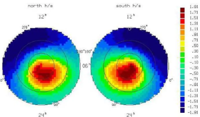
Fig. 1.Dynamo electric field potential distribution in polar geomag-netic coordinate system (latitude-longitude) obtained in the model GSM TIP for 00:00 UT.
block of calculation of electric field and zonal current in the Earth’s ionosphere of the model GSM TIP, and the used al-gorithm of the calculations are explained in every detail.
The equatorial electrojet is essentially a LT (local time) phenomenon with the UT component resulting from longi-tudinal differences arising from the differences in conductiv-ity due to various factors, e.g. the fact that the dipole axis and the geographic axis do not coincide, or that the ambi-ent magnetic field has a non-dipolar componambi-ent, or that the magnetospheric sources are contributing to the electric fields or conductivity. From all listed factors in this work there is only the first factor taken into account, namely, that the dipole axis and the geographic axis do not coincide. The second and the third of the above factors are neglected here. Firstly, in the model GSM TIP the dipole approximation of the ambient geomagnetic field is used, therefore a non-dipol component naturally is neglected. Secondly, all calculations in this work were carried out taking into account the dynamo field generated by thermospheric winds only. Therefore the contribution of electric fields of magnetospheric convection is absent.
The inclusion of the new block of the electric field cal-culation in the model GSM TIP allows us to investigate the equatorial ionosphere. The calculations were carried out for quiet equinox conditions on 22.03.1987 during solar activity minimum (F10.7=76).
3 Calculation results and their discussion
Figure 1 shows the global distribution of the dynamo electric field potential in kV in a polar geomagnetic coordinate sys-tem (latitude-longitude), calculated on the basis of GSM TIP for 00:00 UT. The geomagnetic latitudes are shown by circles with steps of 30◦from the geomagnetic pole to the
Fig. 2.Zonal current linear density obtained in the model GSM TIP in A/km for 23:00 UT.
Fig. 3.Zonal current linear density obtained in the model GSM TIP in A/km for 06:00 UT.
meridians 0◦, 90◦, 180◦and 270◦. Also the time in a
Solar-Magnetospheric coordinate system is shown.
Figures. 2–5 show the global distributions of zonal cur-rent linear density, obtained with the model GSM TIP for 23:00 UT, 06:00 UT, 15:00 UT and 20:00 UT in a Cartesian geomagnetic coordinate system (longitude-latitude). One can see that the maximal intensity of the zonal current linear density has maxima at 23:00 UT and 15:00 UT and minima at 06:00 UT and 20:00 UT. The greatest and smallest val-ues of the equatorial electrojet maximal intensity during the day can differ by a factor of two. The longitudinal extent of the equatorial electrojet area does hardly reveal any UT-variation, although it is possible to note the greatest longitu-dinal extent at 06:00 UT. With amplification of the equatorial electrojet maximal intensity, its latitudinal extent slightly in-creases also (about 5–10◦). At the same time, the equatorial
electrojet in its maxima of intensity has approximately an
Fig. 4.Zonal current linear density obtained in the model GSM TIP in A/km for 15:00 UT.
Fig. 5.Zonal current linear density obtained in the model GSM TIP in A/km for 20:00 UT.
identical width, and in the minima of intensity the electrojet is narrow in the morning and wide in the afternoon.
relation between the hemispheres.
The majority of researchers speak now only about a lon-gitudinal variation of various parameters of the near-Earth environment, including the equatorial electrojet, forgetting about UT-variation or identifying it with a longitudinal vari-ation. We consider this as incorrect. Really, in an experiment it is very difficult, if at all possibly, to separate a longitudi-nal variation from a UT-variation. However it is very easy in numerical modeling.
Let us consider the sources of these variations. Originally it is supposed that a UT variation of the ionospheric param-eters are connected with the mismatch of the axis of the ge-omagnetic dipole with the geographic axis of the Earth rota-tion. For any existence of longitudinal variations the pres-ence of longitudinal sources is necessary. These sources must be located in well-defined places on the Earth’s sur-face. For example, the South-Atlantic anomaly is a source of longitudinal variations. This source is connected with the presence of multipole components in the geomagnetic field. UT and longitude are independent variables. We can expand every function in series of these two independent variables. Herewith one term of the decomposition in the series will de-pend on longitude only, the other will dede-pend on UT only, but the third (the cross terms of the decomposition) will depend on both variables. The UT variation will be described with the terms of the decomposition, depending on UT. The longi-tudinal variation will be described with the terms, depending on longitude. But cross terms will describe a dependency on both UT, and longitude. Most likely, the contribution of these terms will be small in comparison with the contribution of the main terms, describing longitudinal and UT variation. In our model the geomagnetic field is approximated by a central dipole, the axis of which does not coincide with the geographical axis of Earth rotation. In this approximation of a geomagnetic field, there is no non-dipole component. Therefore the visible reasons for an existence of longitudi-nal variations are absent, while the mechanism of formation of a UT-variations is present. Hence, we shall speak about UT-variations, discussing results of the calculations. Also we shall speak about longitudinal variations, discussing ex-perimental data in which UT and longitudinal variations are contained, since in this case we deal with real data.
The equatorial electrojet is known to peak around 11:00– 12:00 LT. In our calculation results the maximum intensity of the equatorial electrojet appears around3=240◦(11:00 LT)
for 23.00 UT, around 3=130◦ (10:40 LT) for 06:00 UT,
around3=0◦(11:00 LT) for 15:00 UT, and around3=280◦
(10:20 LT) for 20:00 UT. As for a displacement of the maxi-mum of the electrojet into the morning sector of LT in com-parison with real experimental data, this can be caused by ne-glecting tides on the bottom boundary of thermosphere and by neglecting the electric field of magnetospheric convection in our calculations.
In papers by L¨uhr et al. (2004), Manoj et al. (2006), Le Mouel et al. (2006) observational data of the equatorial
elec-trojet obtained with the CHAMP satellite were analyzed. The analysis of data has shown, that the equatorial electrojet rep-resents a narrow formation on the geomagnetic equator. The width of the equatorial electrojet equals about 2000 km in the day-time ionosphere. At the same time the maximal in-tensity of the equatorial electrojet was estimated by L¨uhr et al. (2004) as 0.15 A/m on the average, whereas Manoj et al. (2006) obtained 0.04 A/m for the same value. The data of Manoj et al. (2006) correspond to a lower level of solar activity.
Comparing these data with results of our calculations, we can state their satisfactory consent in position and spatial size of the equatorial electrojet. In our calculations the width of the electrojet along latitude turns out a little greater, than in the experiment. This can be explained with the absence of the electric field of magnetospheric convection and the absence of thermospheric tides in our calculations which could lead to a modification of the spatial distribution of the zonal current in the Earth’s ionosphere or with the rough spatial grid in our model. As for the maximal intensity of the equatorial electrojet in our calculations, its value of 35 A/km is very close to the measurements of Manoj et al. (2006).
A comparison of results of our model calculations with experimental data by Le Mouel et al. (2006) has shown, that: 1. Locations of calculated and observed electrojet at 06:00 UT, 08:00 UT and 22:00 UT practically coincide; 2. While in the experiment the longitudinal extent of the equatorial electrojet depends on UT and is minimal for the southern hemisphere, in the results of the model cal-culations the longitudinal extent of the equatorial elec-trojet is constant. This indicates that in the experiment there are sources of longitudinal and of UT variations of the equatorial electrojet (a real geomagnetic field with all features, including the South-Atlantic magnetic anomaly with which the minimal longitudinal extent of the equatorial electrojet in the southern hemisphere is possibly connected). In the model there are only sources of UT variation (dipole geomagnetic field). From this it is possible to draw the conclusion that the variability of the longitudinal extent of the equatorial electrojet is the consequence of a longitudinal variation;
3. In model calculations the counter electrojet is formed both in the morning and in the evening, but in the evening the counter electrojet is much stronger than in the morning. In the experiment the counter electrojet is formed only in the morning. This fact can be explained by the absence of thermospheric tides in the presented calculations.
Fig. 6.Diurnal behavior of the maximal intensity of the equatorial electrojet obtained in the model GSM TIP in A/km.
therefore each point on the abscissa of this plot corresponds to conditions close to noon for various geomagnetic longi-tudes at the geomagnetic equator. It is shown, that there is a precise semidiurnal harmonic in the diurnal behavior of the equatorial electrojet linear density with maxima at 23:00 UT and 15:00 UT and with minima at 06:00 UT and 20:00 UT.
In investigations by Ivers et al. (2003), Doumouya and Co-hen (2004), and Le Mouel et al. (2006) obtained on the basis of observations of the equatorial electrojet with the CHAMP and Ørsted satellites, it was shown that the variability of the equatorial electrojet depends on time and longitude.
Ivers et al. (2003) and Le Mouel et al. (2006) have shown the existence of a quarter-diurnal (six-hour) harmonic in the equatorial electrojet, i.e. the presence of a UT or longitudinal behavior of the equatorial electrojet with four maxima and accordingly four minima. The maximal intensity of the equa-torial electrojet in our calculations shows a semidiurnal har-monic behavior on UT. We used the geographical longitudes of the maxima from Ivers et al. (2003) in geomagnetic longi-tude at the geomagnetic equator. Then we recalculated these longitudes in UT which correspond to noon conditions in points:λ= 0◦–30◦E corresponding to3= 85◦or 11:00 UT;
λ= 90◦–120◦E corresponding to3 = 175◦, or 05:00 UT;
λ= 180◦–220◦E corresponding to3= 270◦, or 22:00 UT;
λ= 260◦–290◦E corresponding to3= 345◦, or 17:00 UT.
Thus we obtain a coincidence of maxima of the equatorial electrojet in the longitudinal rangesλ= 180◦–220◦E (in our
calculations 23:00 UT, and in experiment 22:00 UT) andλ
= 260◦–290◦E (in our calculations 15:00 UT, and in
experi-ment 17:00‘UT).
Le Mouel et al. (2006) have shown that the longitudinal behavior of the maximal intensity of the equatorial electrojet has four maxima and four minima. Three of the four maxima coincide with the maxima in the paper by Ivers et al. (2003).
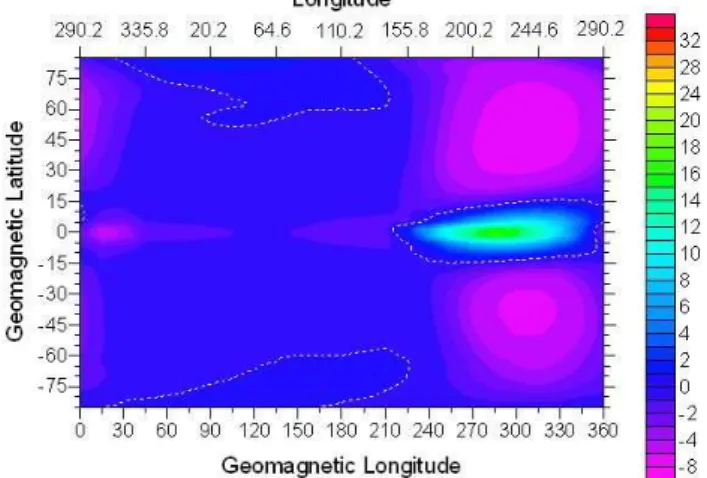
Fig. 7. Zonal current surface density obtained in the model GSM
TIP in A/km2for 23:00 UT.
From the papers by Doumouya and Cohen (2004) it is pos-sible to pick out six extrema in the longitudinal behavior of the intensity of the equatorial electrojet. Three maxima and three minima from their work coincide with three maxima and three minima in the work by Le Mouel et al. (2006).
According to data from Doumouya and Cohen (2004) and Le Mouel et al. (2006) the longitudinal variation of the equa-torial electrojet lays in the range 1.7–2.3 and 2.3–3.2, corre-spondingly. Figure 6 shows, that the magnitude of the UT variation of the equatorial electrojet equals approximately 2 in our calculations. We obtained this magnitude for quiet ge-omagnetic conditions during a spring equinox under a mini-mum of solar activity.
Figures 7–10 show the distributions of zonal current surface density, obtained with the model GSM TIP for 23:00 UT, 06:00 UT, 15:00 UT and 20:00 UT in a Cartesian geomagnetic coordinate system (longitude-altitude). One may notice that its UT-variation is much weaker and equals
∼1–3 A/km2 and herewith the maximal intensity is ∼15– 20 A/km2. At the same time the latitudinal extent of the equa-torial electrojet surface density is maximal at 23:00 UT and 15:00 UT and minimal at 06:00 UT and 20:00 UT.
Fig. 8. Zonal current surface density obtained in the model GSM
TIP in A/km2for 06:00 UT.
Fig. 9. Zonal current surface density obtained in the model GSM
TIP in A/km2for 15:00 UT.
4 Summary
Numerical calculations have shown, that there is a semidi-urnal harmonic in the disemidi-urnal behavior of the maximal
inten-Fig. 10. Zonal current surface density obtained in the model GSM
TIP in A/km2for 20:00 UT.
at 23:00 UT and 15:00 UT and minimal at 06:00 UT and 20:00 UT.
Acknowledgements. The authors express sincere gratitude to
M. F¨orster for useful discussions and for the presentation of our re-ports at the. Kleinheubacher Tagung of the URSI Landesausschuss Deutschland e.V., 2006, Miltenberg, Germany, 25–29 September 2006, thanks to which the opportunity of this publication was given.
References
Baker, W. G. and Martyn, D. F.: Electric Currents in the Ionosphere, I The Conductivity, Phil. Trans. Roy. Soc., London, A246, 281– 294, 1953.
Chapman, S.: The equatorial electrojet as detected from the ab-normal electric current distributions above Huancayo, Peru and elsewhere, Arch. Meteorol. Geophys. Bioklimatol, A4, 368–390, 1951.
Cowling, T. G.: The magnetic field of sunspots, Mon. Not. R. As-tron. Soc., 94, 39–48, 1933.
Doumouya, V. and Cohen, V.: Improving and testing the empiri-cal equatorial electrojet model with CHAMP satellite data, Ann. Geophys., 22. 3323–3333, 2004.
Egedal, J.: The magnetic diurnal variation of the horizontal force near the magnetic equator, Terr. Magn. Atmos. Electr., 52, 449– 451, 1947.
Gershman, B. N.: Dynamics of ionospheric plasmas, Moscow, Nauka, 256p., 1974 (In Russian).
Gurevich, A. V., Krylov, A. L., and Tsedilina, E. E.: Electric Fields in the Earth’s Magnetosphere and Ionosphere, Space Sci. Rev., 19, 59–160, 1976.
Heelis, R. A.: Electrodynamics in the low and middle latitude iono-sphere: a tutorial, J. Atmos. Solar-Terr. Phys., 66, 825–838, 2004.
Ivers, D, Stening, R., Turner, J., et al.: Equatorial electrojet from Ørsted scalar magnetic field observations, J. Geophys. Res., 108, 1061, doi:10.1029/2002JA009310, 2003.
Klimenko, M. V., Klimenko, V. V., and Bruykhanov, V. V.: Com-parison of two variants of model of the electric field in the iono-sphere of the Earth, KSTU News, 8, 59–68, 2005 (In Russian). Klimenko, M. V., Klimenko, V. V., and Bruykhanov, V. V.:
Nu-merical Simulation of the Electric Field and Zonal Current in the Earth’s Ionosphere: The Dynamo Field and Equatorial Electro-jet, Geomagnetism and Aeronomy, 46, 457–466, 2006a.
Klimenko, V. V., Klimenko, M. V., and Bruykhanov, V. V.: Numer-ical modeling of electric field and zonal current in the Earth’s ionosphere – Statement of the problem and test calculations, Matematicheskoye Modelirovaniye, 18, 77–92, 2006b (In Rus-sian).
Korenkov, Yu. N., Klimenko, V. V., Forster, M., et al.: Calculated and observed ionospheric parameters for a Magion 2 passage and EISCAT data on June 31, 1990, J. Geophys. Res., 103, 14 697– 14 710, 1998.
Le Mouel, J.-L., Shebalin, P., and Chuliat, A.: The field of the equa-torial electrojet from CHAMP data, Ann. Geophys., 24, 515– 527, 2006,
http://www.ann-geophys.net/24/515/2006/.
L¨uhr, H., Maus, S., and Rother, M.: Noone-time equatorial electro-jet: Its spatial features as determined by the CHAMP satellite, J. Geophys. Res., 109, A01306, doi:10.1029/2002JA009656, 2004. Manoj, C., L¨uhr, H., Maus, S., et al.: Evidence for short spatial correlation lengths of the noontime equatorial electrojet inferred from a comparison of satellite and ground magnetic data, J. Geo-phys. Res., 111, A11312, doi:10.1029/2006JA011855, 2006. Martyn, D. F., Cowling, T.G., and Borger, R.: Electric conductivity
of the ionospheric D-region, Nature, Lond., 162, 142–143, 1948. Namgaladze, A. A., Korenkov, Yu. N., Klimenko, V. V., et al.: Global Model of the Thermosphere-Ionosphere-Protonosphere System, Pure and Applied Geophysics (PAGEOPH), 127, 219– 254, 1988.
Namgaladze, A. A., Korenkov, Yu. N., Klimenko, V. V., et
al.: Numerical modelling of the thermosphere–ionosphere–
protonosphere system, J. Atmos. Terr. Phys., 53, 1113–1124, 1991.
Richmond, A.D.: Modeling the ionosphere wind dynamo: A re-view, Pure and Appl. Geophys. (PAGEOPH), 131, 413–435, 1989.
Richmond, A. D.: Thermospheric Dynamics and Electrodynam-ics, in Sol.-Terr. Phys., Principles and Theoretical Foundations, edited by: Carovillano, R. L. and Forbes, J. M., D. Reidel Pub-lishing Company, Dordrecht, Holland, 523–607, 1982.
Singh, A., and Cole, K.D.: A Numerical Model of the Ionospheric Dynamo I. Formulation and Numerical Technique, J. Atoms. Terr. Phys., 49, 521–527, 1987.
Stening, R.J.: Modeling the equatorial electrojet, J. Geopys. Res., 90, 1705-1719, 1985.
Sugiura, M. and Cain, J. G.: A Model Equatorial Electrojet, J. Geo-phys. Res., 71, 1869–1877, 1966.
Volland, H.: Atmospheric Electrodynamics, Springer-Verlag,